Energy-level diagrams and their contribution to fifth-order Raman and second-order infrared responses: Distinction between relaxation mechanisms by two-dimensional spectroscopy

Abstract

We develop a Feynman rule for energy-level diagrams emphasizing their connections to the double-sided Feynman diagrams and physical processes in the Liouville space. Thereby we completely identify such diagrams and processes contributing to the two-dimensional response function in the Brownian oscillator model. We classify such diagrams or processes in quartet and numerically present signals separately from each quartet of diagrams or Liouville-space processes. We find that the signal from each quartet is distinctly different from the others; we can identify each peaks in frequency domain with a certain quartet. This offers the basis for analyzing and assigning actual two-dimensional peaks and suggests the possibility of Liouville-space-path selective spectroscopy. As an application we demonstrate an example in which two familiar homogeneous mechanisms of relaxation are distinguished by existence or non-existence of certain peaks on the two-dimensional map; appearance or disappearance of certain peak is sensitive to the coupling mechanism. We also point out some confusion in the literature with regard to inclusion of relaxation effects.

TITLE RUNNING HEAD: Energy-level diagrams and their contribution to 2D spectroscopy

I Introduction

The use of ultrashort laser pulse to probe the properties of molecules has been propelled by the rapid advances in laser measurement techniques.Mukamel Recently, two-dimensional (2D) vibrational spectroscopy has been actively studied, where the spectral properties of multi-body correlation functions of polarizability (2D Raman spectroscopy) TM93 ; COT ; Duppen01 ; KA1 ; GT ; Miller02 ; Saito ; Saito02 ; Fleming02 ; Reichman02 ; Cao02 ; Stratt02 ; Keyes or dipole moment (2D infrared spectroscopy) Hoch98 ; Hamm01 ; Tok01 ; Cho01 are measured. The 2D technique provides information about the inter- and intra-molecular interactions which cause energy relaxations. Mukamel00 ; Fourkas01 ; Cho02 ; Hoch02 ; Wright

Theoretically, optical responses of molecular vibrational motions have been studied mainly by either an oscillator model Oxtoby or energy level model. Redfield The oscillator model utilizes molecular coordinates to describe molecular motions. This description is physically intuitive since optical observables (dipole moments or Raman polarizability) are also described by molecular coordinates; the effects of relaxation, which are caused by interactions of the coordinate with some other degrees of freedom, are rather easy to be included. As long as the potential is harmonic or nearly harmonic, signals can be calculated analytically. TM93 ; OTWANH ; OT ; OTCPL ; CPLfreq ; Suzuki01 ; Suzuki02

On the contrary, the energy-level model employs the energy eigen functions of a molecular motion but is physically equivalent to the oscillator model. Accordingly, laser interactions are described by transitions between the energy levels; the optical processes, including the time-ordering of laser pulses, are conveniently described by diagrams such as Albrecht diagrams, LeeAlbrecht or double-sided Feynman diagrams. Mukamel Although the inclusion of relaxation processes from physical insight is less intuitive and is restricted to some special cases, this model has the advantage in identifying peak positions of optical signal in frequency domain. Steffen ; Fourkas97 ; Tominaga01 ; Tok01b The anharmonicity of potential and nonlinear mode-mode coupling are also easily taken into account. Phase matching conditions, which chose a specific Liouville path contribution by the configuration of Laser beams, Mukamel is also easy to take into account. In the oscillator model or molecular dynamical simulations, the phase matching condition can be done only after calculating entire response functions. KTCPL

The rate of increase in the number of diagrams, however, with the increase of laser interactions is severer in the energy-level model; this becomes serous practical problem for multi-dimensional spectroscopy, where many laser interactions are included. For example, more than 16 diagrams are involved in the lowest order in the third-order anhamonicity in fifth-order Raman while all the diagrams can be represented by a single field-theoretic diagram in the oscillator model. OT

In this paper we try to bridge the two complementary models by transferring some results obtained in the oscillator-model to the energy-level language. Although we lose the simplicity (e.g. small number of diagrams) we gain in an insight into optical processes; we can assign each peaks in certain optical  or Liouville-space processes. The resulting energy-level Feynman rule for the oscillator system allows inclusion of relaxation mechanism in an ad hoc way. As an application, we compare two system with different damping constants. This example reveals that existence of certain peaks in 2D spectroscopic map sensitively depends on the relaxation model.

II Interaction of energy level diagrams

We consider a molecular vibrational motion described by a single molecular coordinate $Q$. In the energy-level representation, the Hamiltonian is expressed as

$$H_{0}=\hbar\Omega\left(a^{{\dagger}}a+\frac{1}{2}\right)$$ (1)

where $a$ and $a^{{\dagger}}$ are the creation and annihilation operators and

$$Q=\sqrt{\frac{\hbar}{2M\Omega}}\left(a+a^{{\dagger}}\right)$$ (2)

for the system with the mass $M$. The energy level of this harmonic system is given by $E_{n}=\hbar\Omega_{n}$ with $\Omega_{n}=(n+1/2)\Omega$ for which we introduce the frequency difference $\Omega_{mn}=\Omega_{m}-\Omega_{n}.$ If the system interacts with the laser field $E(t)$, it is governed by the full Hamiltonian,

$$H(t)=\left\{\begin{array}[c]{cc}H_{0}+\mu E(t)&\text{(IR)}\\ H_{0}+\alpha E(t)^{2}&\text{(Raman)}\end{array}\right.$$ (3)

where $\mu$ is the dipole for infrared (IR) and $\alpha$ is the polarizability for Raman spectroscopy. Both operators can be expanded as

$$x=x_{0}+x_{1}Q+\frac{1}{2!}x_{2}Q^{2}+\frac{1}{3!}x_{3}Q^{3}+\cdots,$$ (4)

We consider the response function, which is pertinent to the 2D second-order IR (for non isotropic media) or the 2D fifth-order Raman spectroscopy,

$$R^{(2)}(T_{1},T_{2})$$

$$=\theta\left(t_{3}-t_{2}\right)\theta\left(t_{2}-t_{1}\right)\left\langle\left[\left[x\left(t_{3}\right),\frac{i}{\hbar}x\left(t_{2}\right)\right],\frac{i}{\hbar}x\left(t_{1}\right)\right]\right\rangle$$

where $x(t)$ is the Heisenberg operator of $x$ for the non-interacting Hamiltonian $H_{0}$ and $\left\langle O\right\rangle\equiv\mathrm{Tr}\left[\rho_{0}O\right]$ with $\rho_{0}=e^{-\beta H_{0}}/\mathrm{Tr}\left[e^{-\beta H_{0}}\right]$ (when we include the effect of dissipation at the level of Hamiltonian, $H_{0}$ includes the bath Hamiltonian and the system-bath interaction). The operator $x$ stands for $\mu$ (IR) or $\alpha$ (Raman). Generalization to the combined IR and Raman cases such as $\left\langle\left[\left[\mu\left(t_{3}\right),\mu\left(t_{2}\right)\right],\alpha\left(t_{1}\right)\right]\right\rangle$ PC ; Chorev ; Wright ; WrightA will also be treated below.

$R^{(2)}(T_{1},T_{2})$ for the harmonic system can be expanded in terms of $Q$ by Eq. (4). The leading order is given as

$$R^{(2)}(T_{1},T_{2})=\left(\frac{i}{\hbar}\right)^{2}\frac{x_{1}^{2}x_{2}}{2}\left(R_{1}+R_{2}+R_{3}\right),$$ (5)

where

$$R_{1} =\left\langle\left[\left[Q^{2}\left(T_{1}+T_{2}\right),Q\left(T_{1}\right)\right],Q\left(0\right)\right]\right\rangle$$

$$R_{2} =\left\langle\left[\left[Q\left(T_{1}+T_{2}\right),Q^{2}\left(T_{1}\right)\right],Q\left(0\right)\right]\right\rangle$$

$$R_{3} =\left\langle\left[\left[Q\left(T_{1}+T_{2}\right),Q\left(T_{1}\right)\right],Q^{2}\left(0\right)\right]\right\rangle.$$

with

$$t_{3}-t_{2} =T_{2}$$ (6)

$$t_{2}-t_{1} =T_{1},$$

II.1 Raman spectroscopy

For the moment, we concentrate on the Raman case, i.e. $\left\langle\left[\left[\alpha\left(t_{3}\right),\alpha\left(t_{2}\right)\right],\alpha\left(t_{1}\right)\right]\right\rangle$. Some of processes in Eq. (5) are represented by the energy-level (Albrecht-like) diagrams in Fig. 1. The differences from the original Albrecht diagram are mentioned at the end of this section. Before explaining diagrams, let us review possible transitions by operators $Q$ and $Q^{2}$; $Q$ can cause a one-quantum excitation or de-excitation while $Q^{2}$ can result in a two-quantum excitation or de-excitation in addition to a zero-quantum transition. For example, from $\left|0\right\rangle\rightarrow Q^{2}\left|0\right\rangle\sim\left[\left(a^{{\dagger}}\right)^{2}+aa^{{\dagger}}\right]\left|0\right\rangle$, we see that by the action of the operator $Q^{2}$, the ground ket state $\left|0\right\rangle$ can be changed into $\left|0\right\rangle$ (zero-quantum transition) or $\left|2\right\rangle$ (two-quantum excitation). In the same way, $\left\langle 2\right|$ can be brought into $\left\langle 0\right|$ (two-quantum de-excitation) or $\left\langle 2\right|$.

In the diagrams, time runs from the left to the right. Each pair of arrows stands for a Raman excitation. The pair with a wavy arrow signifies the Raman induction decay (last interaction); the first interaction occurs at $t_{1}$, the second at $t_{2}$, and the last at $t_{3}$.

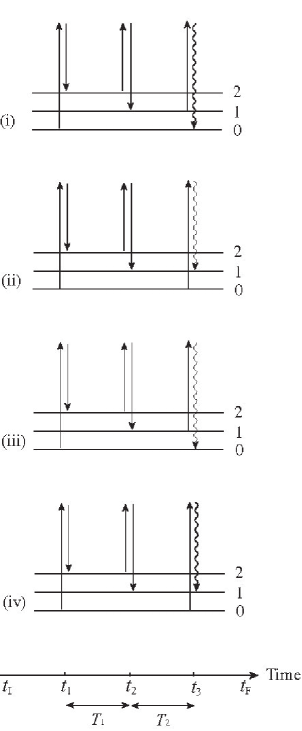
Figure 1: Energy-level diagrams of $R^{(2)}(T_{1},T_{2})$ for Raman processes.

The full description of a quantum state at a certain time requires both the bra state $\left\langle n\right|$ and ket state $\left|m\right\rangle$; at any time the state is fully specified by the Liouville state $\left|m\right\rangle\left\langle n\right|$. In the diagrams, the excitation or de-excitation of the bra state is expressed by a pair of fine arrows while that of the ket state by normal ones. For example, the first interaction at $t_{1}$ of (i) and (ii) is a two-quantum excitation of the ket state while that of (iii) and (iv) is of the bra state.

In the Liouville space, the diagram (i) is interpreted as follows. The system is initially in the ground (Liouville) state $\left|0\right\rangle\left\langle 0\right|$. The first interaction causes a two-quantum excitation of the ket state; $\left|0\right\rangle\left\langle 0\right|\rightarrow\left|2\right\rangle\left\langle 0\right|$ at $t_{1}$. The second interaction causes a one-quantum de-excitation, $\left|2\right\rangle\left\langle 0\right|\rightarrow\left|1\right\rangle\left\langle 0\right|$ at $t_{2}$. The last shows a one-quantum de-excitation, $\left|1\right\rangle\left\langle 0\right|\rightarrow\left|0\right\rangle\left\langle 0\right|$ at $t_{3}$. As a whole, we denote this as

$$\left|0\right\rangle\left\langle 0\right|\underset{t_{1}}{\rightarrow}\left|2\right\rangle\left\langle 0\right|\underset{t_{2}}{\rightarrow}\left|1\right\rangle\left\langle 0\right|\underset{t_{3}}{\rightarrow}\left|0\right\rangle\left\langle 0\right|$$ (7)

The diagram (ii)-(iv) are interpreted as follows:

$$\left|0\right\rangle\left\langle 0\right|\underset{t_{1}}{\rightarrow}\left|2\right\rangle\left\langle 0\right|\underset{t_{2}}{\rightarrow}\left|1\right\rangle\left\langle 0\right|\underset{t_{3}}{\rightarrow}\left|1\right\rangle\left\langle 1\right|$$ (8)

$$\left|0\right\rangle\left\langle 0\right|\underset{t_{1}}{\rightarrow}\left|0\right\rangle\left\langle 2\right|\underset{t_{2}}{\rightarrow}\left|0\right\rangle\left\langle 1\right|\underset{t_{3}}{\rightarrow}\left|0\right\rangle\left\langle 0\right|$$ (9)

$$\left|0\right\rangle\left\langle 0\right|\underset{t_{1}}{\rightarrow}\left|0\right\rangle\left\langle 2\right|\underset{t_{2}}{\rightarrow}\left|0\right\rangle\left\langle 1\right|\underset{t_{3}}{\rightarrow}\left|1\right\rangle\left\langle 1\right|$$ (10)

Note here that a pair of fine arrows always correspond to the excitation or de-excitation of the bra state.

We define the population state by $\left|n\right\rangle\left\langle n\right|$, while the coherence state by $\left|n\right\rangle\left\langle m\right|$ with $n\neq m$. We notice that, after the last interaction, in all of the above 4 diagrams, the system is always in a population state ($\left|0\right\rangle\left\langle 0\right|$ or $\left|1\right\rangle\left\langle 1\right|$). In summary, a diagram does not vanish only when the final state is a population state (Theorem 1). This corresponds to the trace operation in the definition of the response function.

In this paper, we simplify the original Albrecht diagrams LeeAlbrecht for comparison with the Liouville paths. The main differences are the following: (1) we use always the same horizontal lines regardless of ket or bra states; it is not the case in the original Albrecht diagrams and (2) time runs always from left to right in our representation while the direction for the bra and ket states are the opposite in the original version. Our representation is somewhat simpler in that a single diagram in ours corresponding to several diagrams in the original version.

II.2 IR and IR-Raman spectroscopy

IR processes appearing in the IR response function, $\left\langle\left[\left[\mu\left(t_{3}\right),\mu\left(t_{2}\right)\right],\mu\left(t_{1}\right)\right]\right\rangle$, corresponding to Fig. 1-(iv) is described in Fig. 2; each quantum transition is represented not by a pair of arrow but an arrow. Note Raman and IR processes can be equivalent theoretically at this level of description, although even orders of IR processes, such as second-order IR signal vanish except in anisotopic media, such as adsorbed molecules on metallic surface. Chosurface This situation can be overcome by mixing the IR and Raman processes. PC By using narrow-band lasers (two IR excitation pulses followed one probe pulse which create Raman signal) Zhao and Wright demonstrated such experiment. Wright ; WrightA

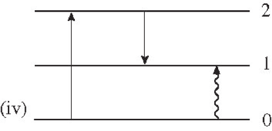
Figure 2: An energy-level diagram of $R^{(2)}(T_{1},T_{2})$ for IR processes.

As an IR-Raman spectroscopy, we consider the response function, $\left\langle\left[\left[\mu\left(t_{3}\right),\mu\left(t_{2}\right)\right],\alpha\left(t_{1}\right)\right]\right\rangle$, for example. A diagram corresponding to Fig.1-(iv) is shown in Fig. 3; Raman and IR transitions are represented by a pair of arrows and an arrow, respectively. Diagrams corresponding to the other IR-Raman response function such as $\left\langle\left[\left[\mu\left(t_{3}\right),\mu\left(t_{2}\right)\right],\alpha\left(t_{1}\right)\right]\right\rangle$ can be described in a similar manner.

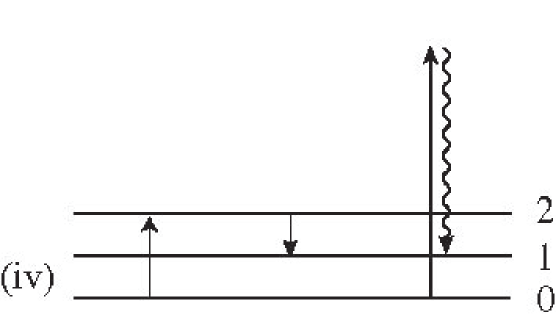
Figure 3: An energy-level diagrams of $R^{(2)}(T_{1},T_{2})$ for IR-Raman processes, $\left\langle\left[\left[\mu\left(t_{3}\right),\mu\left(t_{2}\right)\right],\alpha\left(t_{1}\right)\right]\right\rangle$.

III Energy-level diagram and double-sided diagram

We can represent processes in the Liouville-space in a different way by the double-sided Feynman diagrams. The diagrams in Fig. 4 are the translation of the diagrams in Fig. 1, 2, or 3. In the double-sided diagrams, time runs from the left to the right (as in the energy-level diagram). The horizontal lines, however, are always two in number, the upper and lower line. The former represents the ket state while the latter the bra state. The single circle stands for a one-quantum transition, while the double circle for a two quantum transition. The quantum number of the bra and ket states is denoted explicitly in the diagram.

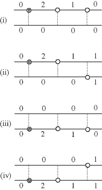
Figure 4: Double-sided Feynman diagrams of $R^{(2)}(T_{1},T_{2})$.

It is noted that there are some differences of diagrammatic notation among articles. For example, in some literature, the quantum transition is not represented by  circles but arrows. In other one, diagrams are rotated by 90 degree so that the time runs from the bottom to the top.

In general, as seen below (VI. A), the double-sided diagram is convenient for enumeration of all possible diagrams while the energy-level diagram is for understanding the physical process.

IV Feynman rules for the diagrams

We have introduced several way to represent optical processes as in Figs. 1-4. It is emphasized here that the interpretation in terms of the Liouville-space state $\left|m\right\rangle\left\langle n\right|$ is unique except for what $x_{k}$ implies. Accordingly, we can develop a universal rule to write down analytical expressions from diagrams via the interpretations (such as Eqs. (7)-(10)) in the Liouville-space; the derivation is a straightforward exercise in elementary quantum mechanics and would be discussed elsewhere. It can be summarized in the following way. We associate with each interaction (originating from the interaction $Q^{k}/k!$) at a certain time or each propagation for a certain period one of the following factors:

$\text{interaction (}n\geq 0\text{)}$	factor
$\left|m\right\rangle\rightarrow\left|m+n\right\rangle$	$\frac{i}{\hbar}x_{k}\left\langle m+n\right|Q^{k}\left|m\right\rangle/k!$
$\left|m\right\rangle\rightarrow\left|m-n\right\rangle$	$\frac{i}{\hbar}x_{k}\left\langle m-n\right|Q^{k}\left|m\right\rangle/k!$
$\left\langle m\right|\rightarrow\left\langle m+n\right|$	$-\frac{i}{\hbar}x_{k}\left\langle m\right|Q^{k}\left|m+n\right\rangle/k!$
$\left\langle m\right|\rightarrow\left\langle m-n\right|$	$-\frac{i}{\hbar}x_{k}\left\langle m\right|Q^{k}\left|m-n\right\rangle/k!$
remark	$\text{omit }\pm\frac{i}{\hbar}\text{ for the last interaction}$

pr$\text{opagation (}t\geq 0\text{)}$	factor
$\text{ }\left|m\right\rangle\left\langle n\right|\text{ for }t$	$e^{-i\zeta_{mn}t-\Gamma_{mn}t}\text{ }$

By multiplying all the factors and putting another factor 1/2 to avoid double-counting (see Theorem 2 below), we obtain an analytical expression of the corresponding diagram (Feynman rule). Here, we have introduced $\zeta_{mn}$ and $\Gamma_{mn}$ $(\geq 0)$ to describe relaxation; the difference of frequency modified due to the relaxation is defined by $\zeta_{mn}=(m-n)\zeta$ while the relaxation constant $\Gamma_{mn}$ for the state $\left|m\right\rangle\left\langle n\right|$ possesses the symmetric property, $\Gamma_{nm}=\Gamma_{mn},$ which is a necessary condition for a consistent theory (see below Eq. (12)). Without dissipation, $\zeta_{mn}\rightarrow\Omega_{mn}=(m-n)\Omega$ and $\Gamma_{mn}\rightarrow 0.$ In the Brownian oscillator model with the damping constant $\gamma$, the corrected frequency $\zeta$ is given by $\zeta=\sqrt{\Omega^{2}-\left(\gamma/2\right)^{2}}$. Grabert ; Weiss The expression for $\Gamma_{mn}$ in this model shall be discussed below.

By definition, the propagation period implies the time between two interactions. This excludes the periods from $t_{I}$ to $t_{1}$ and from $t_{3}$ to $t_{F}$ in diagrams in Figs. 1-4 (or, say, in Eq. (7)-(10)) because there is no interaction at $t_{I}$ or $t_{F}$; we associate the unity for these special period.

Let us apply our rule without relaxation ($\Gamma_{mn}=0$, $\zeta_{mn}=\Omega_{mn}$) to a diagram or a Liouville-space path. As the first example, we consider the diagram (i) (of Fig. 1 or 4). We have only 2 separate propagation periods by definition. In the first period from $t_{1}$ to $t_{2}$ the system is in the state $\left|2\right\rangle\left\langle 0\right|$ and thus we have the factor $e^{-i\Omega_{20}\left(t_{2}-t_{1}\right)}$ while for the last period from $t_{2}$ to $t_{3}$ the system is in the state $\left|1\right\rangle\left\langle 0\right|$ and we have the factor $e^{-i\Omega_{10}\left(t_{3}-t_{2}\right)}$; in total we have the propagation factor, $e^{-i\Omega_{20}T_{1}}\cdot e^{-i\Omega_{10}T_{2}}$, where we have used the relation (6). In addition, as the result of the three interactions, we have other factors, $\frac{i}{\hbar}x_{2}\left\langle 2\right|Q^{2}\left|0\right\rangle/2\cdot\frac{i}{\hbar}x_{1}\left\langle 1\right|Q\left|2\right\rangle\cdot x_{1}\left\langle 0\right|Q\left|1\right\rangle=\left(\frac{i}{\hbar}\frac{\hbar}{2M\Omega}x_{1}\right)^{2}x_{2}$ (Note here the relations, Eq. (2) as well as, $a\left|n\right\rangle=\sqrt{n}\left|n-1\right\rangle,$ and $a^{{\dagger}}\left|n\right\rangle=\sqrt{n+1}\left|n+1\right\rangle$). In summary, the process in Eq. (7) or the diagram (i) is given (with the extra factor 1/2 associate with double-counting) by

$$(\text{i})=\left(\frac{i}{\hbar}\right)^{2}\frac{x_{1}^{2}x_{2}}{2}\left(\frac{\hbar}{2M\Omega}\right)^{2}e^{-i2\Omega T_{1}}\cdot e^{-i\Omega T_{2}}$$ (11)

The process in Eq. (8) or the diagram (ii) (of Figs. 1 or 4) is different from (i) only after $t_{3}$. Although the last interaction at $t_{3}$ is that for the bra state (expressed by the fine arrows and different form (i)) the factors for this last interaction is the same with that of (i) by the above Feynman rule; there is no sign differences between bra and ket states (only) for the last interaction. In summary we have

$$(\text{ii})=(\text{i}).$$

In general, we have the following theorem, which is related to the double counting: The diagrams different only by the side of the last interaction (bra or ket side) have the same contribution (Theorem2).

The process in Eq. (9) or in the diagram (iii) can be estimated in a similar manner by the above Feynman rule:

$$(\text{iii})=\left(-\frac{i}{\hbar}\right)^{2}\frac{x_{1}^{2}x_{2}}{2}\left(\frac{\hbar}{2M\Omega}\right)^{2}e^{i2\Omega T_{1}}\cdot e^{i\Omega T_{2}}.$$

Note here that the sign in front of $i/\hbar$ is minus because of the interactions on the bra state (fine arrows). From $t_{1}$ to $t_{2}$, the system is in the states $\left|0\right\rangle\left\langle 2\right|$ and $\left|2\right\rangle\left\langle 0\right|$ in (iii) and (i), respectively; these two states are the complex-conjugate of each other. From $t_{2}$ to $t_{3}$, the state of (iii) ($\left|0\right\rangle\left\langle 1\right|$) is again in the complex-conjugate state of (i) ($\left|1\right\rangle\left\langle 0\right|$). Accordingly, (iii) given in the above is the complex conjugate of (i), i.e.,$($iii$)=($i$)^{\ast}$. Diagrammatically, in (iii) of Fig. 1, all the normal arrows in (i) are replaced by the fine arrows. In general, The complex-conjugate diagram is obtained by interchanging all the normal and fine arrows (Theorem 3). In the double-sided Feynman diagrams, instead, The complex-conjugate diagram is obtained by interchanging the circles on the upper and lower lines (Theorem 3^′).

The diagram (iv) is the complex-conjugate diagram of (ii) because the fine and normal arrows are interchanged, i.e., $($iv$)=($ii$)^{\ast}.$ We can also verify the relation, $($iii$)=($iv$)$, from the above Feynman rule with reconfirming Theorem 2.

V Temperature effect and initial state

In the above, we have assumed the system is initially in the ground state $\left|0\right\rangle\left\langle 0\right|$, which is usually justified for high frequency vibration modes at a room temperature. For high temperatures or low frequency modes, however, excited states $\left|n\right\rangle\left\langle n\right|$ are initially populated according to the Boltzmann factor. In general, we have to estimate all the possible processes assuming that the system is initially in the population state $\left|n\right\rangle\left\langle n\right|$ using the above mentioned rule, and then summing up with respect to $n$ with the Boltzmann factor $e^{-\beta E_{n}}/\sum_{n}e^{-\beta E_{n}}$ (in the case without dissipation); this completes our Feynman rule.

Even if we take into account the contribution from general initial state $\left|n\right\rangle\left\langle n\right|$, however, in the (fully-corrected) Ohmic Brownian oscillator model, we still have the same result with above as shown in the previous literature. This is the reflection of the relation

$$\left\langle n\right|X\left|n\right\rangle=\left\langle 0\right|X\left|0\right\rangle$$

where $X$ is some special combination of operators (This could be directly checked by laborious calculation by using our Feynman rule). The fact that $R^{(2)}(T_{1},T_{2})$ treated in this paper is independent of the temperature and thus we can obtain a finite temperature result even if assuming that the system is initially in the ground state is by no means trivial but established by other calculation methods. OT This implies, for example, that the dependence on $n$ of the analytical expression corresponding to Fig. 5 cancels out with some other diagram. When the damping mechanism other than (fully-corrected) Ohmic Brownian oscillator model, our results presented below might be interpreted as an high frequency approximation, i.e. $\hbar\Omega\gg kT$.

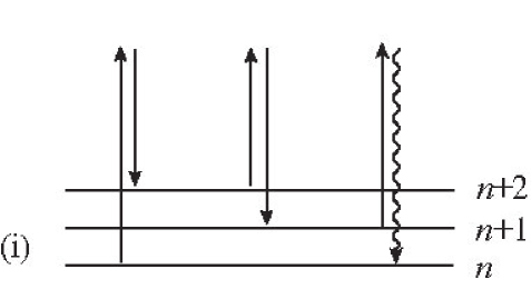
Figure 5: General process corresponding to Fig. 1 (i)

VI Liouville-space quartet

The four diagrams (i)-(iv) in Figs. 1 and 4 are a special set in the sense that we can obtain the other three, starting from one of the quartet.

In the energy-level diagram, we obtain the second by changing the last interaction by using one of the following rule (depending on the last interaction of the starting diagram); (1) the ket excitation to a bra de-excitation, (2) the ket de-excitation to a bra excitation, (3) the bra excitation to a ket de-excitation and (4) the bra de-excitation to a ket excitation. The remaining two diagrams are the complex-conjugate diagrams of the previous two diagrams where the conjugates are obtained by interchanging the fine and normal arrows.

In the double-sided diagram the second diagram is obtained by lowering or raising the last circle. The remaining two is by interchanging lower and upper line with circles.

As seen before, the corresponding analytical expressions of (i)-(iv) have the relations, $($i$)=($ii$),$ $($iii$)=($iv$),$ and $($i$)=($iii$)^{\ast}.$ The sum of the quartet is always real:

$$(\text{i})+(\text{ii})+(\text{iii})+(\text{iv})=4\operatorname{Re}[(\text{i})]=4\operatorname{Re}[(n)]$$

where $n=$ i, ii, iii or iv. Taking the real part of Eq. (11)  we have an expression for the quartet,

$$V_{I}=-\frac{x_{1}^{2}x_{2}}{2\left(M\Omega\right)^{2}}\cos\left(2\Omega T_{1}+\Omega T_{2}\right)$$ (12)

In terms of the interpretation in the Liouville space in Eqs. (7)-(10), all the processes posses a common property; the two-quantum coherence ($\left|2\right\rangle\left\langle 0\right|$ or $\left|0\right\rangle\left\langle 2\right|$) is realized for $T_{1}$ while the one-quantum coherence ($\left|1\right\rangle\left\langle 0\right|$ or $\left|0\right\rangle\left\langle 1\right|$) for $T_{2}$; we denote this as:

$$\left|2\right\rangle\left\langle 0\right|\rightarrow\left|1\right\rangle\left\langle 0\right|\text{ and }\left|0\right\rangle\left\langle 2\right|\rightarrow\left|0\right\rangle\left\langle 1\right|$$

This is reflected by the factor $\cos\left(2\Omega T_{1}+\Omega T_{2}\right)$ in Eq. (12).

We notice that in the case with damping if $\Gamma_{mn}$ (and $\zeta_{mn}$) were not symmetric, $V_{I}$ could not be real; the symmetric property of $\Gamma_{mn}$ is required for the response function to be real.

VI.1 Quartets representation: all possible quartets for $R^{(2)}(T_{1},T_{2})$

We show six quartets R(1)$-$R(6) in Fig. 6 in the double-sided representation. The square brackets imply the quartet; only one of the quartet is explicitly written in the bracket. For example, R(1) of Fig. 6 collectively stands for (i)-(iv) of Fig. 4.

In Fig. 6, on the right side, ten quartets in the energy-level representation are given; some quartets in double-sided representation corresponds to not one but two quartets in the energy-level representation. For example, R(1) contains contribution I and I^′, while R(3) contains only A2.

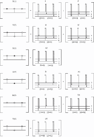
Figure 6: All possible quartets for $R^{(2)}(T_{1},T_{2})$. The square bracket implies that four diagrams are collectively represented. For example, the first diagram in the energy-level diagram for R(1) corresponds to not only (i) of Fig. 1 (which is explicitly written in the bracket) but other three diagrams (ii)-(iv) of Fig. 1.

These six quartets R(1)$-$R(6) in Fig. 6 exhaust all possible contribution to the right-hand side of Eq. (5); there are 3 ways for the position of the double quantum transition (double circle) and there $2^{3}$ ways to put the three (including one double circle) circles upper or lower line, which leads to $3\cdot 2^{3}$ double-sided Feynman diagrams in total. These $3\cdot 8$ diagrams can be divided into $6$ quartets that have been shown. We understand here that the double-sided diagram is convenient for enumerating all possible diagrams.

VI.2 Estimation of quartets

The analytical expression of quartet II is given via our Feynman rule:

II $$=4\operatorname{Re}\left[-\left(\frac{i}{\hbar}\right)^{2}\left(\frac{\hbar}{2M\zeta}\right)^{2}\right.$$ (13)

$$\times\left.\frac{x_{1}^{2}x_{2}}{2}\cdot e^{-i2\zeta T_{1}-\Gamma_{20}T_{1}}\cdot e^{-i\zeta T_{2}-\Gamma_{21}T_{2}}\right],$$ (14)

where the analytical expression in the square bracket has been derived from the diagram explicitly drawn in the bracket in Fig. 6 (in the presence of dissipation). For example, the propagator $e^{-i2\zeta T_{1}-\Gamma_{20}T_{1}}$ and $e^{-i\zeta T_{2}-\Gamma_{21}T_{2}}$ come from the propagation of $\left|2\right\rangle\left\langle 0\right|$ and $\left|2\right\rangle\left\langle 1\right|$, respectively.

In this way we obtain the expression:

$$R^{(2)}\left(T_{1},T_{2}\right)=\text{I}+\text{II}+\text{A}+\text{B}+\text{C}+\text{D1+D2}$$ (15)

with

I $$=-\frac{x_{1}^{2}x_{2}}{2\left(M\zeta\right)^{2}}e^{-\Gamma_{20}T_{1}-\Gamma_{10}T_{2}}\cos\left(2\zeta T_{1}+\zeta T_{2}\right)$$

II $$=\frac{x_{1}^{2}x_{2}}{2\left(M\zeta\right)^{2}}e^{-\Gamma_{20}T_{1}-\Gamma_{21}T_{2}}\cos\left(2\zeta T_{1}+\zeta T_{2}\right)$$

A $$=-\frac{x_{1}^{2}x_{2}}{2\left(M\zeta\right)^{2}}e^{-\Gamma_{10}T_{1}-\Gamma_{10}T_{2}}\cos\left(\zeta T_{1}+\zeta T_{2}\right)$$

B $$=\frac{x_{1}^{2}x_{2}}{2\left(M\zeta\right)^{2}}e^{-\Gamma_{10}T_{1}-\Gamma_{12}T_{2}}\cos\left(\zeta T_{1}-\zeta T_{2}\right)$$

C $$=-\frac{x_{1}^{2}x_{2}}{2\left(M\zeta\right)^{2}}e^{-\Gamma_{10}T_{1}-\Gamma_{20}T_{2}}\cos\left(\zeta T_{1}+2\zeta T_{2}\right)$$

D1 $$=-\frac{1}{4}\frac{x_{1}^{2}x_{2}}{\left(M\zeta\right)^{2}}e^{-\Gamma_{10}T_{1}-\Gamma_{00}T_{2}}\cos\left(\zeta T_{1}\right)$$

D2 $$=\frac{3}{4}\frac{x_{1}^{2}x_{2}}{\left(M\zeta\right)^{2}}e^{-\Gamma_{10}T_{1}-\Gamma_{11}T_{2}}\cos\left(\zeta T_{1}\right)$$

As for the derivation of this we remark: (1) Quartets I’ and II’ cancel out because I’$=-\frac{1}{4}\frac{x_{1}^{2}x_{2}}{\left(M\zeta\right)^{2}}e^{-\Gamma_{00}T_{1}-\Gamma_{10}T_{2}}\cos\left(\zeta T_{2}\right)$ and II’$=\frac{1}{4}\frac{x_{1}^{2}x_{2}}{\left(M\zeta\right)^{2}}e^{-\Gamma_{00}T_{1}-\Gamma_{01}T_{2}}\cos\left(\zeta T_{2}\right)$ (The numerical factor 1/4 can be understood from the first two-quantum transition associated with $\left\langle 0\right|Q^{2}\left|0\right\rangle\varpropto\left\langle 0\right|aa^{{\dagger}}\left|0\right\rangle=1$). (2) The sum A2+A1 reduces to A (The numerical factor for A2 (or A1) can be estimated by noting the second two-quantum transition $\left\langle 1\right|Q^{2}\left|1\right\rangle\varpropto\left\langle 1\right|aa^{{\dagger}}+a^{{\dagger}}a\left|1\right\rangle=3$ (or $\left\langle 0\right|Q^{2}\left|0\right\rangle\varpropto\left\langle 0\right|aa^{{\dagger}}\left|0\right\rangle=1$)).

It is worth while observing the relationships between analytical expressions and the symbolic interpretations of the remaining quartets:

A $$\text{: }\left|1\right\rangle\left\langle 0\right|\rightarrow\left|1\right\rangle\left\langle 0\right|\text{ and }\left|0\right\rangle\left\langle 1\right|\rightarrow\left|0\right\rangle\left\langle 1\right|$$

B $$\text{: }\left|1\right\rangle\left\langle 0\right|\rightarrow\left|1\right\rangle\left\langle 2\right|\text{ and }\left|0\right\rangle\left\langle 1\right|\rightarrow\left|2\right\rangle\left\langle 1\right|$$

C $$\text{: }\left|1\right\rangle\left\langle 0\right|\rightarrow\left|2\right\rangle\left\langle 0\right|\text{ and }\left|0\right\rangle\left\langle 1\right|\rightarrow\left|0\right\rangle\left\langle 2\right|$$

D2 $$\text{: }\left|1\right\rangle\left\langle 0\right|\rightarrow\left|1\right\rangle\left\langle 1\right|\text{ and }\left|0\right\rangle\left\langle 1\right|\rightarrow\left|1\right\rangle\left\langle 1\right|$$

D1 $$\text{: }\left|1\right\rangle\left\langle 0\right|\rightarrow\left|0\right\rangle\left\langle 0\right|\text{ and }\left|0\right\rangle\left\langle 1\right|\rightarrow\left|0\right\rangle\left\langle 0\right|$$

That is, we can associate the state $\left|n\right\rangle\left\langle m\right|$ with $\zeta_{n,m}$ and $\Gamma_{mn}$.

In addition, if we fully include the temperature effect by our Feynman rule with tracking all the possible processes, we could obtain the result given in Appendix B of Steffen .

VII Damping mechanism

We can confirm that the well-known result for the Ohmic Brownian oscillator (BO) model (Ohmic implies that the system-bath coupling is in the bilinear form) is reproduced from Eq. (15) by setting

$$\text{ }\Gamma_{nm}=\left\{\begin{array}[c]{cc}\gamma&\text{for }\left|n\right\rangle\left\langle n\right|\\ \left|n-m\right|\gamma/2&\text{for }\left|n\right\rangle\left\langle m\right|\text{ (}n\neq m\text{)}\end{array}\right.\text{ }$$ (16)

where $\left|m\right|$ represents the absolute value of $m$. Actually, in the Brownian result, I+II should be zero, which is true if $\Gamma_{21}=\Gamma_{10}$, while D1+D2 should be $-2\cdot$D1, which is true if $\Gamma_{11}=\Gamma_{00}$; $\Gamma_{mn}$ in Eq. (16) satisfies these requirements.

The cancellation of I and II is one of the feature of the Brownian result. Another feature is that the state $\left|0\right\rangle\left\langle 0\right|$ decays with the relaxation constant $\gamma/2$ which is the same as that for $\left|1\right\rangle\left\langle 1\right|$. These characteristics have intrigued some controversy as mentioned below.

The relaxation constant for the same Ohmic model within the lower level approximation, i.e., at the level of the Fermi’s golden rule with a somewhat ad hoc approximation (see below), given by Steffen ; Fourkas95

$$\Gamma_{mn}=\frac{n+m}{2}\gamma,$$ (17)

which is also simple but incompatible with the above two requirements ($\Gamma_{21}=\Gamma_{10}$ and $\Gamma_{11}=\Gamma_{00}$). With this relaxation constant, I and II survives, for example. (In addition, there is no frequency shift ($\zeta_{mn}\rightarrow\Omega_{mn}$) in this finite-order approximation).

The frequency shift and appearance of the absolute value ($\left|n-m\right|$), which is non-analytic, in the off diagonal relaxation constant in the fully corrected expressions originate from the summation of infinite number of diagrams; in the well-known result of Ohmic BO model the bilinear coupling between the system-bath is fully taken into account; this is the exact prediction from a simple reasonable model and we concern with the relaxation of fully-dressed states in the exact result of BO model. On the contrary, the relaxation constant in Eq. (17), is the result of the same model but with the second-order (in the coupling strength) approximation. Nonetheless in some context the second-order result has been favored while the full-order result has been questioned. Cho ; Steffen

As we show below we can distinguish the above two models ((16) or (17)) by some two-dimensional experiment by checking existence or absence of certain peaks. In other words, whether the coherence (off-diagonal) relaxation constant which depends only on the quantum number difference (where $\Gamma_{m+n,m}=\Gamma_{n,0}$) and the level independent population relaxation is appropriate (as the first-order picture) or not might be checked experimentally.

Note that if the system has some sort of anharmonicity such as the anharmonicity of potential Oxtoby or the nonlinear system-bath coupling KT , the relaxation constants do not hold the relation $\Gamma_{21}=\Gamma_{10}$ etc., even we take into account higher-order system bath interactions. Then the number of Liouville paths involved in the optical processes increase dramatically especially when the system-bath interaction is very strong. Also if the laser-molecular interaction is much shorter than the time duration of the system-bath interactions, one has to regard the relaxation rate as a function of time, i.e. $\Gamma_{nm}(t)$. In such case, the equation of motion approach is more appropriate than the diagrammatic approaches, although it requires computationally expensive calculations. 40 ; T ; ST ; TS KT KTnew

We comment on confusion in the literature with regard to the Redfield theory, one example of which is Eq. (17). The Redfield theory without the rotational wave approximation (RWA) is equivalent to the Fokker-Planck equation. 40 ; T ; ST ; TS ; KT ; KTnew The time evolution operator in the Liouville space from the state $\left|\left.k,l\right\rangle\right\rangle\equiv\left|k\right\rangle\left\langle l\right|$ to $\left\langle\left\langle i,j\right.\right|\equiv$ $\left\langle i\right|\cdots\left|j\right\rangle$ is then expressed as $\left\langle\left\langle i,j\right.\right|e^{-i\left(\hat{H}^{\times}-\hat{\Gamma}\right)t}\left|\left.k,l\right\rangle\right\rangle$, where $\hat{H}^{\times}$ is the quantum Liouvillian and $\hat{\Gamma}$ is the damping operator (Redfield operator). In energy-level representation, $\left|\left.k,l\right\rangle\right\rangle$ is the eigen-function of the Hamiltonian but not the eigen function of $\hat{\Gamma}$, which makes difficult to evaluate this propagator. However, one sometimes “reads off” the damping constant directly from the Redfield tensor elements $\Gamma_{ijkl}$ and incorporate them in the propagator as $\left\langle\left\langle i,j\right.\right|e^{-i\left(\hat{H}^{\times}-\Gamma_{ijkl}\right)t}\left|\left.k,l\right\rangle\right\rangle$, which can not be justified from the coordinate representation model. Steffen ; Fourkas95 Accordingly, this ad hoc methodology possesses a flaw in the sense that the theory thus obtained does not converges to analytical perturbative results such as obtained by the Brownian oscillator model. It is possible to evaluate effective tensor element $\Gamma_{ijkl}^{(\text{eff})}$ by solving the equation of motion such as the Fokker-Planck equation with linear and nonlinear system-bath interactions, 40 ; T ; ST ; TS ; KT ; KTnew but the calculated results are quite different from the Redfield tensor elements. KT

VIII Multi-mode system

Extension to the multi-mode system, whose characteristic modes are represented by $\left\{Q_{s}\right\}$, $\left\{M_{s}\right\}$, and $\left\{\gamma_{s}\right\}$, is straightforward. CPLfreq ; TokPRL Tominaga01 ; Tok01 We expand the dipole or polarizability operator as

$$x=x_{0}+\sum_{s}x_{1}^{(s)}Q^{(s)}+\frac{1}{2!}\sum_{s,s^{\prime}}x_{2}^{(ss^{\prime})}Q^{(s)}Q^{(s^{\prime})}+\cdots,$$

and we denote the Liouville state by

$$\left|\left\{n_{s}\right\}\right\rangle\left\langle\left\{n^{\prime}\right\}\right|=\left(\left|n_{1}\right\rangle\left\langle n_{1}^{\prime}\right|\right)_{1}\cdots\left(\left|n_{s}\right\rangle\left\langle n_{s}^{\prime}\right|\right)_{s}\cdots,$$

where $\left\{n_{s}\right\}=(n_{1},n_{2},\cdots)$ is the quantum-number of the corresponding mode. Here and hereafter, we use the notation in which $\left|n_{s},n_{s^{\prime}}\right\rangle\left\langle m_{s},m_{s^{\prime}}\right|$ stands for the state where the mode $s$ and $s^{\prime}$ are in the states $\left|n_{s}\right\rangle\left\langle m_{s}\right|$ and $\left|n_{s^{\prime}}\right\rangle\left\langle m_{s^{\prime}}\right|$, respectively. For example, $\left|0,1\right\rangle\left\langle 2,3\right|$ means that the first and the second modes are in the ground and the first excited ket states while they are in the second and the third excited bra state, respectively.

The factor (in the Feynman rule) for the transition is well explained by example. The transition,

$$\left|0,0\right\rangle\left\langle 0,0\right|\rightarrow\left|2,1\right\rangle\left\langle 0,0\right|$$

caused by the operator $\left(Q^{(1)}\right)^{2}Q^{(2)}$ is associated with the factor $\frac{i}{\hbar}\left(x_{3}^{(112)}+x_{3}^{(121)}+x_{3}^{(211)}\right)\left\langle 2,1\right|\left(Q^{(1)}\right)^{2}Q^{(2)}\left|0,0\right\rangle/3!=\frac{i}{\hbar}x_{3}^{(112)}\sqrt{2}\frac{\hbar}{M_{1}\Omega_{1}}\sqrt{\frac{\hbar}{M_{2}\Omega_{2}}}/2!$ while the transition (again caused by $\left(Q^{(1)}\right)^{2}Q^{(2)}$),

$$\left|0,0\right\rangle\left\langle 0,0\right|\rightarrow\left|0,0\right\rangle\left\langle 2,1\right|$$

is associated with the same factor with the minus sign. If the above transition occurs at the last time, however, we have to omit the factor $i/\hbar$ as in the single-mode case.

Note here that the transition of the type,

$$\left|0,0\right\rangle\left\langle 0,0\right|\rightarrow\left|1,0\right\rangle\left\langle 1,0\right|$$

cannot occur at once, but

$$\left|0,0\right\rangle\left\langle 0,0\right|\rightarrow\left|1,1\right\rangle\left\langle 0,0\right|$$

can occur; bra and ket excitation can never occur simultaneously, that is, the simultaneous multi-transition can occur exclusively for the ket state or for the bra state.

The time propagation factor of each mode in the state $\left(\left|n\right\rangle\left\langle m\right|\right)_{s}$ during a (positive) time duration $t$ is given by $e^{-i(n-m)\Omega_{s}t}$ for the harmonic system without dissipation.

In the multi-mode case, the diagram explicitly written in the square bracket D2 in Fig. 6 represents either a single-mode process,

$$\left\{\begin{array}[c]{cc}\left|1\right\rangle\left\langle 0\right|\rightarrow\left|1\right\rangle\left\langle 1\right|&\text{(mode }s\text{)}\\ \text{---}\rightarrow\text{---}&\text{(mode }s^{\prime}\text{)}\end{array}\right.,$$

where — implies no time propagation, or a two-mode process,

$$\left\{\begin{array}[c]{cc}\left|1\right\rangle\left\langle 0\right|\rightarrow\left|1\right\rangle\left\langle 0\right|&\text{(mode }s\text{)}\\ \text{---}\rightarrow\left|0\right\rangle\left\langle 1\right|&\text{(mode }s^{\prime}\text{)}\end{array}\right.,$$ (18)

which is explicitly shown in the square braket D2 in Fig. 7.

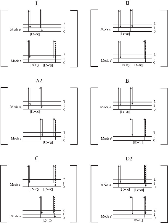
Figure 7: Two-mode processes. It should be noted that there are no counterparts of I’, II’, A1, D1.

In other words, in the multi-mode case, quartet D2 in Fig. 6 represents the quartets displayed in Fig. 8.

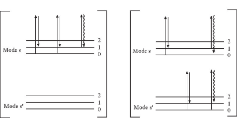
Figure 8: Quartets represented by the quartet (D) of Fig. 6.

By use of the above rules in the multi-mode case, we see that the propagator of the process in Eq. (18) is given by $e^{-i\Omega_{s}T_{1}}\cdot e^{-i\left(\Omega_{s}-\Omega_{s^{\prime}}\right)T_{2}}$because $\left|1,0\right\rangle\left\langle 0,0\right|$ propagates for $T_{1}$ and $\left|1,0\right\rangle\left\langle 0,1\right|$ for $T_{2}$. The remaining interaction factors are $\frac{i}{\hbar}x_{1}^{(s)}\left\langle 1,0\right|Q^{(s)}\left|0,0\right\rangle\cdot\left(-\frac{i}{\hbar}\right)x_{1}^{(s^{\prime})}\left\langle 0,0\right|Q^{(s^{\prime})}\left|0,1\right\rangle\cdot\left(x_{2}^{(ss^{\prime})}+x_{2}^{(s^{\prime}s)}\right)\left\langle 0,1\right|Q^{(s)}Q^{(s^{\prime})}\left|1,0\right\rangle/2!$ (and the factor 1/2 to avoid double counting). Taking into account the other elements of the quartets, we obtain the total contribution D2 of Fig. 6 in the multi-mode case in a form:

D2 $$=4\sum_{s,s^{\prime}}\operatorname{Re}\left[-\frac{1}{2}c_{ss^{\prime}}\left(\frac{i}{\hbar}\right)^{2}x_{1}^{(s)}x_{1}^{(s^{\prime})}x_{2}^{(ss^{\prime})}\right.$$ (19)

$$\left.\frac{\hbar}{2M_{s}\Omega_{s}}\frac{\hbar}{2M_{s^{\prime}}\Omega_{s^{\prime}}}e^{-i\Omega_{s}T_{1}}e^{-i\left(\Omega_{s}-\Omega_{s^{\prime}}\right)T_{2}}\right]$$

where $c_{ss^{\prime}}$ is 1 and 3/2 for $s\neq s^{\prime}$ and for $s=s^{\prime},$ respectively. Comparing this with diagrams we learn that we should associate $\left|n_{s},n_{s^{\prime}}\right\rangle\left\langle m_{s},m_{s^{\prime}}\right|$ with $\Omega_{n_{s}m_{s}}^{(s)}+\Omega_{n_{s^{\prime}}m_{s^{\prime}}}^{(s^{\prime})}$. These 4 quartets correspond to 4 diagrams in Fig. 8 (in the dissipation-less case).

In this way (taking into account the effect of dissipation), we have

$$R^{(2)}\left(T_{1},T_{2}\right)$$ (20)

$$=\sum_{s=1,2}\left(\text{I}_{s}+\text{II}_{s}+\text{B}_{s}+\text{C}_{s}+\text{D1}_{s}+\text{D2}_{2}\right)$$

$$+\sum_{s,s^{\prime}}\text{A2}_{ss^{\prime}}+\left.\sum_{s,s^{\prime}}\right.^{\prime}\left(\text{B}_{ss^{\prime}}+\text{C}_{ss^{\prime}}+\text{D}_{ss^{\prime}}\right),$$

where the prime in the expression, $\sum_{s,s^{\prime}}^{\prime}$ , implies that the terms with $s=s^{\prime}$ are excluded in the sum. Here, each term is given by:

$$\text{I}_{s} =-f_{ss}e^{-\Gamma_{20}^{(s)}T_{1}-\Gamma_{10}^{(s)}T_{2}}\cos\left(2\zeta_{s}T_{1}+\zeta_{s}T_{2}\right)$$

$$\text{II}_{s} =f_{ss}e^{-\Gamma_{20}^{(s)}T_{1}-\Gamma_{21}^{(s)}T_{2}}\cos\left(2\zeta_{s}T_{1}+\zeta_{s}T_{2}\right)$$

$$\text{A2}_{ss^{\prime}} =-f_{ss^{\prime}}e^{-\Gamma_{10}^{(s)}T_{1}-\Gamma_{10}^{(s^{\prime})}T_{2}}\cos\left(\zeta_{s}T_{1}+\zeta_{s^{\prime}}T_{2}\right)$$

$$\text{B}_{s} =f_{ss}e^{-\Gamma_{10}^{(s)}T_{1}-\Gamma_{12}^{(s)}T_{2}}\cos\left(\zeta_{s}T_{1}-\zeta_{s}T_{2}\right)$$

$$\text{B}_{ss^{\prime}} =f_{ss^{\prime}}e^{-\Gamma_{10}^{(s)}T_{1}-\Gamma_{01}^{(s^{\prime})}T_{2}}\cos\left(\zeta_{s}T_{1}-\zeta_{s^{\prime}}T_{2}\right)$$

$$\text{C}_{s} =-f_{ss}e^{-\Gamma_{10}^{(s)}T_{1}-\Gamma_{20}^{(s)}T_{2}}\cos\left(\zeta_{s}T_{1}+2\zeta_{s}T_{2}\right)$$

$$\text{C}_{ss^{\prime}} =-f_{ss^{\prime}}e^{-\Gamma_{10}^{(s)}T_{1}-\left(\Gamma_{10}^{(s)}+\Gamma_{10}^{(s^{\prime})}\right)T_{2}}$$

$$\times\cos\left(\zeta_{s}T_{1}+\left(\zeta_{s}-\zeta_{s^{\prime}}\right)T_{2}\right)$$

$$\text{D1}_{s} =-\frac{1}{2}f_{ss}e^{-\Gamma_{10}^{(s)}T_{1}-\Gamma_{00}^{(s)}T_{2}}\cos\left(\zeta_{s}T_{1}\right)$$

$$\text{D2}_{s} =\frac{3}{2}f_{ss}e^{-\Gamma_{10}^{(s)}T_{1}-\Gamma_{11}^{(s)}T_{2}}\cos\left(\zeta_{s}T_{1}\right)$$

$$\text{D2}_{ss^{\prime}} =-f_{ss^{\prime}}e^{-\Gamma_{10}^{(s)}T_{1}-\left(\Gamma_{10}^{(s)}+\Gamma_{10}^{(s^{\prime})}\right)T_{2}}$$

$$\times\cos\left(\zeta_{s}T_{1}+\left(\zeta_{s}-\zeta_{s^{\prime}}\right)T_{2}\right)$$

with

$$f_{ss^{\prime}}=\frac{x_{1}^{(s)}x_{1}^{(s^{\prime})}x_{2}^{(ss^{\prime})}}{2M_{s}\zeta_{s}M_{s^{\prime}}\zeta_{s^{\prime}}}.$$

We remark the following: (1) I${}_{ss^{\prime}}$ and II${}_{ss^{\prime}}$ always cancel out while I_s and II_s cancel out only if

$$\Gamma_{10}^{(s)}=\Gamma_{21}^{(s)}.$$

(2) The sum $\left(\text{A1}+\text{A2}\right)_{s}$ is just given by setting $s^{\prime}\rightarrow s$ in A2${}_{ss^{\prime}}$. (3) When we put

$$\text{ }\Gamma_{nn}^{(s)} =\gamma_{s}/2\text{ for }\left|n_{s}\right\rangle\left\langle n_{s}\right|$$

$$\Gamma_{mn}^{(s)} =\left|n_{s}-m_{s}\right|\gamma_{s}/2\text{ for }\left|n_{s}\right\rangle\left\langle m_{s}\right|\text{ (}n_{s}\neq m_{s}\text{),}$$ (21)

the above expression reduces to the result of the fully corrected Brownian oscillator model. If we employ the model with the relaxation constant,

$$\Gamma_{mn}^{(s)}=\frac{n+m}{2}\gamma_{s}$$

this leads a different result; one of the feature is the survival of the single mode terms I_s and II${}_{s}.$

IX Feynman rule in frequency domain

In the frequency domain, we study the quantity

$$\int_{0}^{\infty}d\omega_{1}\int_{0}^{\infty}d\omega_{2}\,e^{i\omega_{1}T_{1}+i\omega_{2}T_{2}}R^{(2)}(T_{1},T_{2})$$

The frequency domain expression is obtained by using the above propagators in frequency domain (or, instead, directly by Fourier transformation of Eq. (20)). The general propagating factor in the multi-mode case, $e^{-\Gamma T_{1}-i\Omega T_{1}}\cdot e^{-\Gamma^{\prime}T_{2}-i\Omega^{\prime}T_{2}},$ is, in the frequency domain, replaced by

$$\frac{i}{\omega_{1}-\Omega+i\Gamma}\cdot\frac{i}{\omega_{2}-\Omega^{\prime}+i\Gamma^{\prime}}.$$ (22)

X 2D signal from each Liouville-space quartet

In this section, we present two-dimensional signals from each Liouville-space quartet separately in the fully corrected Brownian oscillator model. In the frequency domain, since the signal is a complex number, we show the absolute value of the signal. In the time domain, the signal is real, which is directly shown.

X.1 Frequency Domain

X.1.1 Single weakly-damped mode

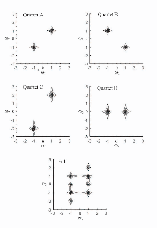
Figure 9: Contour plot of the signal from the system with a single mode with weak damping. The upper four plots correspond to the separate contribution from each Liouville-space quartets. The bottom plot is the sum of them, i.e., the total signal.

Fig. 9 shows signals from the system with a single mode ($\Omega=1$, $\gamma=0.1$, in arbitrary unit). Signals from each Liouville space quartet are separately shown. We can interpret each peak in the following way: the process represented by $\left|n\right\rangle\left\langle m\right|\rightarrow\left|n^{\prime}\right\rangle\left\langle m^{\prime}\right|$ imply that the system is in the state $\left|n\right\rangle\left\langle m\right|$ for $T_{1}$ and $\left|n^{\prime}\right\rangle\left\langle m^{\prime}\right|$ for $T_{2}$; we assign $\Omega_{nm}$ and $\Gamma_{nm}$ for $T_{1}$ and $\Omega_{n^{\prime}m^{\prime}}$ and $\Gamma_{n^{\prime}m^{\prime}}$ for $T_{2}$. This can be symbolically written as

$$\left|n\right\rangle\left\langle m\right|\rightarrow\left|n^{\prime}\right\rangle\left\langle m^{\prime}\right|\Rightarrow\left\{\begin{array}[c]{c}\left(\Omega_{nm},\Omega_{n^{\prime}m^{\prime}}\right)\\ \left(\Gamma_{nm},\Gamma_{n^{\prime}m^{\prime}}\right)\end{array}\right..$$

Actually, the process $\left|n\right\rangle\left\langle m\right|\rightarrow\left|n^{\prime}\right\rangle\left\langle m^{\prime}\right|$ corresponds to the peak at the position at $(\omega_{1},\omega_{2})=\left(\Omega_{nm},\Omega_{n^{\prime}m^{\prime}}\right)$ with the width in the $\omega_{1}$-axis and $\omega_{2}$-axis given by $\Gamma_{nm}$ and $\Gamma_{n^{\prime}m^{\prime}}$, respectively. This results from the expression in Eq. (22) and can be confirmed numerically as we see below.

We note here that we need not consider the contribution from the quartets I and II because they cancels out with each other in the fully corrected Brownian oscillator model.

Quartets A=A1+A2: this be symbolized by $\left|1\right\rangle\left\langle 0\right|\rightarrow\left|1\right\rangle\left\langle 0\right|$ and its complex conjugate $\left|0\right\rangle\left\langle 1\right|\rightarrow\left|0\right\rangle\left\langle 1\right|$. The former process can be symbolically written as

$$\left|1\right\rangle\left\langle 0\right|\rightarrow\left|1\right\rangle\left\langle 0\right|\Rightarrow\left\{\begin{array}[c]{c}\left(\Omega_{10},\Omega_{10}\right)\\ \left(\Gamma_{10},\Gamma_{10}\right)\end{array}\right.\Rightarrow\left\{\begin{array}[c]{c}\left(\Omega,\Omega\right)\\ \left(\gamma/2,\gamma/2\right)\end{array}\right..$$

This suggests a diagonal peak $(\omega_{1},\omega_{2})=(\Omega,\Omega)$ whose widths in the $\omega_{1}$-direction and $\omega_{2}$-direction are both $\gamma/2$; this peak shows symmetric pattern with respect to the two axis, which can be seen in the contour plot in Fig. 9. With the complex conjugate process $\left|0\right\rangle\left\langle 1\right|\rightarrow\left|0\right\rangle\left\langle 1\right|$, we associate

$$\left|1\right\rangle\left\langle 0\right|\rightarrow\left|1\right\rangle\left\langle 0\right|\Rightarrow\left\{\begin{array}[c]{c}\left(\Omega_{01},\Omega_{01}\right)\\ \left(\Gamma_{01},\Gamma_{01}\right)\end{array}\right.\Rightarrow\left\{\begin{array}[c]{c}-\left(\Omega,\Omega\right)\\ \left(\gamma/2,\gamma/2\right)\end{array}\right..$$

Namely, the quartet pair A corresponds to two symmetric diagonal peaks at $(\omega_{1},\omega_{2})=\pm(\Omega,\Omega)$ (see the top left plot of Fig. 9).

Quartet B: symbolically, the association is as follows:

$$\left|1\right\rangle\left\langle 0\right|\rightarrow\left|1\right\rangle\left\langle 2\right|\Rightarrow\left\{\begin{array}[c]{c}\left(\Omega_{10},\Omega_{12}\right)\\ \left(\Gamma_{10},\Gamma_{12}\right)\end{array}\right.\Rightarrow\left\{\begin{array}[c]{c}\left(\Omega,-\Omega\right)\\ \left(\gamma/2,\gamma/2\right)\end{array}\right.$$

and its complex conjugate

$$\left|0\right\rangle\left\langle 1\right|\rightarrow\left|2\right\rangle\left\langle 1\right|\Rightarrow\left\{\begin{array}[c]{c}\left(\Omega_{01},\Omega_{21}\right)\\ \left(\Gamma_{01},\Gamma_{21}\right)\end{array}\right.\Rightarrow\left\{\begin{array}[c]{c}\left(-\Omega,\Omega\right)\\ \left(\gamma/2,\gamma/2\right)\end{array}\right.$$

Namely, we have two symmetric diagonal peaks at $(\omega_{1},\omega_{2})=\pm(\Omega,-\Omega)$ (see the top right of Fig. 9).

Quartet C: in the similar way, from the association

$$\left|1\right\rangle\left\langle 0\right|\rightarrow\left|2\right\rangle\left\langle 0\right|\Rightarrow\left\{\begin{array}[c]{c}\left(\Omega_{10},\Omega_{20}\right)\\ \left(\Gamma_{10},\Gamma_{20}\right)\end{array}\right.\Rightarrow\left\{\begin{array}[c]{c}\left(\Omega,-2\Omega\right)\\ \left(\gamma/2,\gamma\right)\end{array}\right.$$

and its conjugate, we should have two significant overtone peaks at $(\omega_{1},\omega_{2})=\pm(\Omega,2\Omega)$ whose width in the $\omega_{1}$-direction is one half of that in the $\omega_{2}$-direction; the peak is elongated in the second axis as can be seen in the contour plot in Fig. 9 (see the middle left of Fig. 9).

Quartet D=D1+D2: from the association,

D2 $$\text{: }\left|1\right\rangle\left\langle 0\right|\rightarrow\left|1\right\rangle\left\langle 1\right|\Rightarrow\left\{\begin{array}[c]{c}\left(\Omega_{10},\Omega_{11}\right)\\ \left(\Gamma_{10},\Gamma_{11}\right)\end{array}\right.\Rightarrow\left\{\begin{array}[c]{c}\left(\Omega,0\right)\\ \left(\gamma/2,\gamma\right)\end{array}\right.$$

D1 $$\text{: }\left|1\right\rangle\left\langle 0\right|\rightarrow\left|0\right\rangle\left\langle 0\right|\Rightarrow\left\{\begin{array}[c]{c}\left(\Omega_{10},\Omega_{00}\right)\\ \left(\Gamma_{10},\Gamma_{00}\right)\end{array}\right.\Rightarrow\left\{\begin{array}[c]{c}\left(\Omega,0\right)\\ \left(\gamma/2,\gamma\right)\end{array}\right.$$

and their complex conjugate, we should have two significant elongated axial peaks at $(\omega_{1},\omega_{2})=(\pm\Omega,0)$ (see the middle right of Fig. 9).

The total signal displayed at the bottom of the Fig. 9 shows 8 significant peaks; now that we completely know from which Liouville-space path each peak originates, we can assign each peak with distinct Liouville-space paths by the following table.

quartet	peak positions in $(\omega_{1},\omega_{2})$ plane
(A)	$\left(\Omega,\Omega\right),\left(-\Omega,-\Omega\right)$
(B)	$\left(\Omega,-\Omega\right),\left(-\Omega,\Omega\right)$
(C)	$\left(\Omega,2\Omega\right),\left(-\Omega,-2\Omega\right)$
(D)	$\left(\Omega,0\right),\left(-\Omega,0\right)$

In Fig. 9, we notice that peaks from quartets (C) and (D) are elongated in the second axis. This point is also understood in the above argument, from which we have the following table.

quartet	width of peaks for $(\omega_{1},\omega_{2})$
(A),(B)	$\left(\gamma,\gamma\right)$
(C),(D)	$\left(\gamma,2\gamma\right)$

X.1.2 Double modes (weak damping)

Fig. 10 shows signals from the system with two weak damping modes ($\Omega_{1}=1$, $\gamma_{1}=0.1\Omega_{1}$, $\Omega_{2}=0.5$, $\gamma_{2}=0.1\Omega_{2}$, in arbitrary unit, with the assumption, $x_{i}^{(s)}=M_{s}=1$, i.e., $f_{ss^{\prime}}=\left(\zeta_{s}\zeta_{s^{\prime}}\right)^{-1}$.). Signals from each Liouville-space quartet are separately shown. We can interpret each signal in the following way.

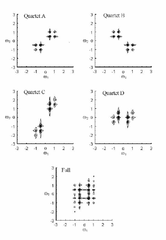
Figure 10: Contour plot of the signal from the system with two weakly-damped modes.

Top-left plot of Fig. 10: Two-mode quartet A2 in Fig. 7 is associated with

$$\left\{\begin{array}[c]{cc}\left|1\right\rangle\left\langle 0\right|\rightarrow\text{---}&\text{(mode }s\text{)}\\ \text{---}\rightarrow\left|1\right\rangle\left\langle 0\right|&\text{(mode }s^{\prime}\text{)}\end{array}\right.\Rightarrow\left\{\begin{array}[c]{c}\left(\Omega_{10}^{(s)},\Omega_{10}^{(s^{\prime})}\right)\\ \left(\Gamma_{10}^{(s)},\Gamma_{10}^{(s^{\prime})}\right)\end{array}\right.$$

and its complex conjugate; this quartet produces the four cross peaks at $(\omega_{1},\omega_{2})=\pm(\Omega_{1},\Omega_{2})$, $\pm(\Omega_{2},\Omega_{1})$. The remaining four diagonal peaks at $(\omega_{1},\omega_{2})=\pm(\Omega_{1},\Omega_{1})$ and $\pm(\Omega_{2},\Omega_{2})$ originate from the single-mode quartets A2 and A1 in Fig. 6, which corresponds to the process

$$\left\{\begin{array}[c]{cc}\left|1\right\rangle\left\langle 0\right|\rightarrow\left|1\right\rangle\left\langle 0\right|&\text{(mode }s\text{)}\\ \text{---}\rightarrow\text{---}&\text{(mode }s^{\prime}\text{)}\end{array}\right.$$

and its conjugate. The widths in the $\omega_{1}$-direction and $\omega_{2}$-direction for the peak at $(\omega_{1},\omega_{2})=\pm(\Omega_{s},\Omega_{s^{\prime}})$ are $\Gamma_{10}^{(s)}$ and $\Gamma_{10}^{(s^{\prime})}$, respectively. In the fully-corrected BO model they are $\gamma_{s}/2$ and $\gamma_{s^{\prime}}/2$, respectively. Although there exists the effect of interferences, the relative size of the width is consistent with this indication. For example, this is the reason the peak at (1,0.5) and (0.5, 1) are elongated in the $\omega_{1}$ and $\omega_{2}$ axes, respectively. In summary, in the fully-corrected BO model, the positions of peaks and two-component of widths are given by

A2/A1 (single-mode) $$\text{: }\left\{\begin{array}[c]{c}\pm(\Omega_{1},\Omega_{1})\text{ with }(\gamma_{1}/2,\gamma_{1}/2)\\ \pm(\Omega_{2},\Omega_{2})\text{ with }(\gamma_{2}/2,\gamma_{2}/2)\end{array}\right.$$

A2 (two-mode) $$\text{: }\left\{\begin{array}[c]{c}\pm(\Omega_{1},\Omega_{2})\text{ with }(\gamma_{1}/2,\gamma_{2}/2)\\ \pm(\Omega_{2},\Omega_{1})\text{ with }(\gamma_{2}/2,\gamma_{1}/2)\end{array}\right.$$

Top-right plot of Fig. 10: Single-mode quartet B in Fig. 6 and two-mode quartet B in 7 are associated with

$$\left\{\begin{array}[c]{cc}\left|1\right\rangle\left\langle 0\right|\rightarrow\left|1\right\rangle\left\langle 2\right|&\text{(mode }s\text{)}\\ \text{---}\rightarrow\text{---}&\text{(mode }s^{\prime}\text{)}\end{array}\right. \Rightarrow\left\{\begin{array}[c]{c}\left(\Omega_{10}^{(s)},\Omega_{12}^{(s^{\prime})}\right)\\ \left(\Gamma_{10}^{(s)},\Gamma_{12}^{(s^{\prime})}\right)\end{array}\right.$$

$$\left\{\begin{array}[c]{cc}\left|1\right\rangle\left\langle 0\right|\rightarrow\text{---}&\text{(mode }s\text{)}\\ \text{---}\rightarrow\left|0\right\rangle\left\langle 1\right|&\text{(mode }s^{\prime}\text{)}\end{array}\right. \Rightarrow\left\{\begin{array}[c]{c}\left(\Omega_{10}^{(s)},\Omega_{01}^{(s^{\prime})}\right)\\ \left(\Gamma_{10}^{(s)},\Gamma_{01}^{(s^{\prime})}\right)\end{array}\right.$$

The single-mode quartet produces the four diagonal peaks in the top-right plot, while the two-mode quartet the four cross peaks. The widths in the two directions for the diagonal peaks are given by $\left(\Gamma_{10}^{(s)},\Gamma_{12}^{(s^{\prime})}\right)$ while those for the cross peaks by $\left(\Gamma_{10}^{(s)},\Gamma_{12}^{(s^{\prime})}\right)$. In summary, we have

B (single-mode): $$\left\{\begin{array}[c]{c}\pm(\Omega_{1},-\Omega_{1})\text{ with }(\gamma_{1}/2,\gamma_{1}/2)\\ \pm(\Omega_{2},-\Omega_{2})\text{ with }(\gamma_{2}/2,\gamma_{2}/2)\end{array}\right.$$

B (two-mode): $$\left\{\begin{array}[c]{c}\pm(\Omega_{1},-\Omega_{2})\text{ with }(\gamma_{1}/2,\gamma_{2}/2)\\ \pm(\Omega_{2},-\Omega_{1})\text{ with }(\gamma_{2}/2,\gamma_{1}/2)\end{array}\right.$$

Middle-left plot of Fig. 10: Single-mode quartet C in Fig. 6 and two-mode quartet C in 7 are associated with

$$\left\{\begin{array}[c]{cc}\left|1\right\rangle\left\langle 0\right|\rightarrow\left|2\right\rangle\left\langle 0\right|&\text{(mode }s\text{)}\\ \text{---}\rightarrow\text{---}&\text{(mode }s^{\prime}\text{)}\end{array}\right. \Rightarrow\left\{\begin{array}[c]{c}\left(\Omega_{10}^{(s)},\Omega_{20}^{(s^{\prime})}\right)\\ \left(\Gamma_{10}^{(s)},\Gamma_{20}^{(s^{\prime})}\right)\end{array}\right.$$

$$\left\{\begin{array}[c]{cc}\left|1\right\rangle\left\langle 0\right|\rightarrow\left|1\right\rangle\left\langle 0\right|&\text{(mode }s\text{)}\\ \text{---}\rightarrow\left|1\right\rangle\left\langle 0\right|&\text{(mode }s^{\prime}\text{)}\end{array}\right. \Rightarrow\left\{\begin{array}[c]{c}\left(\Omega_{10}^{(s)},\Omega_{10}^{(s)}+\Omega_{10}^{(s^{\prime})}\right)\\ \left(\Gamma_{10}^{(s)},\Gamma_{10}^{(s)}+\Gamma_{01}^{(s^{\prime})}\right)\end{array}\right.$$

The single-mode quartet produces the four overtone peaks in the middle-left plot while the two-mode quartet the four cross peaks. In summary, we have

C (single-mode): $$\left\{\begin{array}[c]{c}\pm(\Omega_{1},2\Omega_{1})\text{ with }(\gamma_{1}/2,\gamma_{1})\\ \pm(\Omega_{2},2\Omega_{2})\text{ with }(\gamma_{2}/2,\gamma_{2})\end{array}\right.$$

C (two-mode): $$\left\{\begin{array}[c]{c}\pm(\Omega_{1},\Omega_{1}+\Omega_{2})\text{ with }(\gamma_{1}/2,\left(\gamma_{1}+\gamma_{2}\right)/2)\\ \pm(\Omega_{2},\Omega_{2}+\Omega_{1})\text{ with }(\gamma_{2}/2,\left(\gamma_{1}+\gamma_{2}\right)/2)\end{array}\right.$$

Middle-right plot of Fig. 10: Single-mode quartets D1 and D2 in Fig. 6 are associated with

$$\left\{\begin{array}[c]{cc}\left|1\right\rangle\left\langle 0\right|\rightarrow\left|0\right\rangle\left\langle 0\right|&\text{(mode }s\text{)}\\ \text{---}\rightarrow\text{---}&\text{(mode }s^{\prime}\text{)}\end{array}\right. \Rightarrow\left\{\begin{array}[c]{c}\left(\Omega_{10}^{(s)},\Omega_{00}^{(s^{\prime})}\right)\\ \left(\Gamma_{10}^{(s)},\Gamma_{00}^{(s)}\right)\end{array}\right.$$

$$\left\{\begin{array}[c]{cc}\left|1\right\rangle\left\langle 0\right|\rightarrow\left|1\right\rangle\left\langle 1\right|&\text{(mode }s\text{)}\\ \text{---}\rightarrow\text{---}&\text{(mode }s^{\prime}\text{)}\end{array}\right. \Rightarrow\left\{\begin{array}[c]{c}\left(\Omega_{10}^{(s)},\Omega_{11}^{(s)}\right)\\ \left(\Gamma_{10}^{(s)},\Gamma_{11}^{(s)}\right)\end{array}\right.$$

while two-mode quartet D2 in 7 are associated with

$$\left\{\begin{array}[c]{cc}\left|1\right\rangle\left\langle 0\right|\rightarrow\left|1\right\rangle\left\langle 0\right|&\text{(mode }s\text{)}\\ \text{---}\rightarrow\left|0\right\rangle\left\langle 1\right|&\text{(mode }s^{\prime}\text{)}\end{array}\right.\Rightarrow\left\{\begin{array}[c]{c}\left(\Omega_{10}^{(s)},\Omega_{10}^{(s)}-\Omega_{10}^{(s^{\prime})}\right)\\ \left(\Gamma_{10}^{(s)},\Gamma_{10}^{(s)}+\Gamma_{01}^{(s^{\prime})}\right)\end{array}\right.$$

The single-mode quartet produces the four axial peaks in the middle-right plot while the two-mode quartet the four cross peaks. In summary, we have

D1/D2 (single-mode): $$\left\{\begin{array}[c]{c}\pm(\Omega_{1},0)\text{ with }(\gamma_{1}/2,\gamma_{1})\\ \pm(\Omega_{2},0)\text{ with }(\gamma_{2}/2,\gamma_{2})\end{array}\right.$$

D2 (two-mode): $$\left\{\begin{array}[c]{c}\pm(\Omega_{1},\Omega_{1}-\Omega_{2})\text{ with }(\frac{\gamma_{1}}{2},\frac{\gamma_{1}+\gamma_{2}}{2})\\ \pm(\Omega_{2},\Omega_{2}-\Omega_{1})\text{ with }(\frac{\gamma_{2}}{2},\frac{\gamma_{1}+\gamma_{2}}{2})\end{array}\right.$$

Note here in the fully-corrected BO model, we have $\Gamma_{00}^{(s)}=\Gamma_{11}^{(s)}$ so that the widths from the single-mode quartets D1 and D2 are the same in the above.

The total signal is displayed at the bottom of the figure; we can assign each peak with distinct Liouville-space paths or energy-level diagrams (as in Fig. 8).

X.2 Time domain

Figs. 11 shows the contour plots of peaks from each quartet for a single over-damped mode system. Each quartet contributes to the total signal rather different way. This suggests the possibility of Liouville-space-path selective spectroscopy.

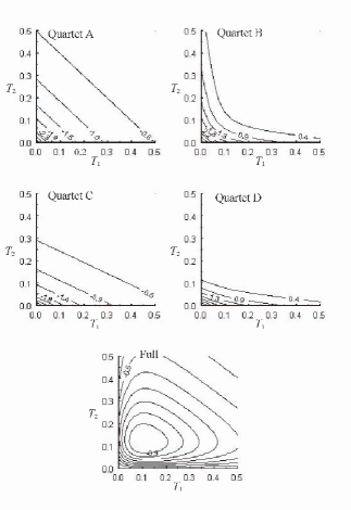
Figure 11: Contour plot of the signal from the system with a single over-damped mode.

XI Signals from Brownian oscillator model and Redfield-type model

In Fig. 12, we compare results from two models: (1) Brownian oscillator (BO) model (the system-bath interaction is fully taken into account) where we put Eq. (16). (2) Redfield-type model (RT) where we put Eq. (17) with the replacement $\zeta_{s}\rightarrow\Omega_{s}$ (no frequency shift).

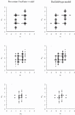
Figure 12: 2D signal from the two models. Top: single mode, $\Omega_{1}=1$. Middle: two modes, $\Omega_{1}=1$, $\Omega_{2}=0.5$. Bottom: two modes, $\Omega_{1}=1.2$, $\Omega_{2}=0.3$. Depending on parameters, the difference between the models manifests as existence or non-existence of diagonal peaks.

Top: the right plot from RT model has extra peaks at on the left (BO) at $(\omega_{1},\omega_{2})=\pm(2,1)$. They originate from the survival of the quartets I and II in Fig. 6.

Middle: on the left plot (BO) there exist extra peaks at $(\omega_{1},\omega_{2})=\pm(1,-1)$. This corresponds to the single-mode quartet B in Fig. 6. For this process, the relaxation constants associated with the $\omega_{2}$-axis, $\Gamma_{12}$, in BO and RT are given by $\gamma$ and $3\gamma$, respectively; the relaxation in RT is much faster, which explains the disappearance of the peaks. The peaks at $(\omega_{1},\omega_{2})=\pm(0.5,-0.5)$ still survives because these peaks not only come from the single-mode process B: in this case, the peaks from quartet I and II overlap with those from other quartets.

Bottom: on the right plot (RT) exists extra peaks at $(\omega_{1},\omega_{2})=\pm(0.3,0.6)$. They corresponds to the survival of I and II in Fig. 6.

In summary, the detailed situation depends on parameters. However, they have one thing in common; the difference between the models manifests as existence or absence of certain peaks. In the numerical results given above are all in the weak damping regime ($\gamma\sim 0.1\Omega$). The weak effect, nonetheless, affects the existence and absence of certain peaks. This is because the damping constants directly matter in the cancellation mechanism of certain processes. Note that the situation is completely different for weak potential anharmonicity or nonlinear polarizability. Such weak effects, on the contrary, do not concern delicate cancellation mechanisms.

If the system exhibits non-weak anharmonicity of potential or the nonlinear system-bath coupling, as mentioned before, there may be the peaks at the similar position predicted by the Redfield-type model. Such mechanism, however, affect not only the existence of these peak but also the entire profile of signal, which involves different Liouville paths. The careful study of the signal in frequency domain shall be the critical test of the Redfield-type model.

XII Concluding remarks

We stated an interpretation of the energy-level diagrams in the Liouville space and summarize the relationships between several diagrammatic representations. We emphasized all the diagrammatic representation reduces to unique interpretations in Liouville space, via which we can write down analytical expression by a Feynman rule.

We have given examples in which each Liouville process make distinctly unique contribution to two-dimensional signal; the selective detection of quantum process by ultrafast spectroscopy might be possible, for example, by utilizing the phase matching condition. KTCPL By suitably prepared spectroscopic configuration, we might be able to concentrate on a certain quantum processes, which allows simpler analysis and more quantitative understanding. Such Liouville-space-path selective spectroscopy might be promising. As photon echo can be distinguished from the pump-probe via phase matching condition, we could differentiate spectroscopic methods by the peaks they produce.

Energy-level diagram is useful in interpreting the physical process but it is so only after confirming the diagram certainly makes a non-zero contribution possibly by other method. For example, in the (fully-corrected) Brownian oscillator model, we can assume the initial state of the diagram is the ground state; this is because we know that other initial states result in the same contribution from a separate calculation. Another example is the cancellation of I by II of Fig. 6.

In this respect, diagram in the field-theoretical context, for example, introduced in OT has some advantage. Number of the diagram to be consider is considerably smaller and analytical expression is much simply obtained; in the case of $R^{(2)}(T_{1},T_{2})$, we have only to consider just two diagrams in total each being given by the product of two certain propagators. This is because the cancellation is always automatically taken into account in this method and, in addition, quartets are summed up from the beginning in a simpler form. However, this conceals physical processes in the Liouville space.

Note here that we have to carefully check out all possible cancellations even if we incorporate the phase matching conditions into the response function, as have been utilized in the electronically resonant experiments such as photon echo and pump-probe to detect the different contributions of the Liouville paths by choosing the laser wavevectors and frequencies. Mukamel This is because in vibrational spectroscopy such as IR echo, the time durations of laser pulses are much shorter than the time periods of molecular vibrations. KTCPL In addition, if the initial temperature of the system is higher than the excitation energy of vibrational levels (as in the case of low frequency modes), or if the nonlinearity of the dipole or Raman transitions are important, Fleming02 ; Saito02 ; OT we have to include a number of Liouville paths especially in higher order spectroscopy; the assignment of the peaks to some Liouville paths become nontrivial.

As for the mechanism of relaxation, we have only considered the system bilinearly coupled with bath. We constructed the Feynman rule by starting from the rule in the case without damping and then by replacing the propagator so that it causes damping with an appropriate choice of the relaxation parameters $\Gamma_{mn}$. One may think that the set $\{\Gamma_{mn}\}$ is an arbitrary set of parameters to fit experimental data; in the case of vibrational spectroscopy, however, $\Gamma_{mn}$’s have to satisfy certain universal relationships, for example, to satisfy the detailed balance condition. In addition, the validity of the rotating wave approximation (RWA) and the Markovian approximation associated with the second order perturbation of the system-bath interaction might become questionable in vibrational spectroscopy; the characterization of the relaxation processes by simple rate constants such as $T_{1}$ and $T_{2}$ might not work. Note here that, although there are some restrictions, one can calculate the signals without using such approximations for Brownian model even in the anharmonic case. OTWANH ; OT ; T ; Suzuki02 In order to verify the consistency of theory, it is important to compare the results from energy level models and the Brownian motion model where the latter is based upon a microscopic picture.

In order to demonstrate how approximations for relaxation processes can change the results, we presented the 2D signals from the Redfield-type model and (full-order) Brownian Oscillator model, and we observed that two models give peaks at different positions even for weak damping. This, in turn, suggests high sensitivity to the damping mechanism of 2D spectroscopy. This situation is in good contrast with cross peaks associated with mode-coupling of anharmonic or nonlinear origin. They might be fairly strong to be observable with stronger diagonal peaks. On the contrary, the cancellation mechanism is subtle and, thus, weak damping effect can cause a drastic difference.

One of the purposes of our paper is to bridge the two complementary approaches of the coorinate-based and the energy-level based models. The results allow us a useful interpretation of the coordinate-based model in the energy-level language. We should note, however, that this interpretation becomes precise only in the weak damping limit. Nonetheless, we believe that it is useful to have a common interpretation for the two approaches in certain situations.

*

Appendix A Expression for $R^{(2)}(\omega_{1},\omega_{2})$

$2R^{(2)}(\omega_{1},\omega_{2})$ is given by Eq. (20) with each term expressed as

$$\text{I}_{s} =\frac{f_{ss}}{\left(\omega_{1}-z_{20}^{(s)}\right)\left(\omega_{2}-z_{10}^{(s)}\right)}+\frac{f_{ss}}{\left(\omega_{1}+\left[z_{20}^{(s)}\right]^{\ast}\right)\left(\omega_{2}+\left[z_{10}^{(s)}\right]^{\ast}\right)}$$

$$\text{II}_{s} =-\frac{f_{ss}}{\left(\omega_{1}-z_{20}^{(s)}\right)\left(\omega_{2}-z_{21}^{(s)}\right)}-\frac{f_{ss}}{\left(\omega_{1}+\left[z_{20}^{(s)}\right]^{\ast}\right)\left(\omega_{2}+\left[z_{21}^{(s)}\right]^{\ast}\right)}$$

$$\left(\text{A2}\right)_{ss^{\prime}}=\frac{f_{ss^{\prime}}}{\left(\omega_{1}-z_{10}^{(s)}\right)\left(\omega_{2}-z_{10}^{(s^{\prime})}\right)}+\frac{f_{ss^{\prime}}}{\left(\omega_{1}+\left[z_{10}^{(s)}\right]^{\ast}\right)\left(\omega_{2}+\left[z_{10}^{(s)}\right]^{\ast}\right)}$$

$$\text{B}_{s} =-\frac{f_{ss}}{\left(\omega_{1}-z_{10}^{(s)}\right)\left(\omega_{2}-z_{12}^{(s)}\right)}-\frac{f_{ss}}{\left(\omega_{1}+\left[z_{10}^{(s)}\right]^{\ast}\right)\left(\omega_{2}+\left[z_{12}^{(s)}\right]^{\ast}\right)}$$

$$\text{B}_{ss^{\prime}} =-\frac{f_{ss^{\prime}}}{\left(\omega_{1}-z_{10}^{(s)}\right)\left(\omega_{2}-z_{01}^{(s^{\prime})}\right)}-\frac{f_{ss^{\prime}}}{\left(\omega_{1}+\left[z_{10}^{(s)}\right]^{\ast}\right)\left(\omega_{2}+\left[z_{01}^{(s)}\right]^{\ast}\right)}$$

$$\text{C}_{s} =\frac{f_{ss}}{\left(\omega_{1}-z_{10}^{(s)}\right)\left(\omega_{2}-z_{20}^{(s)}\right)}+\frac{f_{ss}}{\left(\omega_{1}+\left[z_{10}^{(s)}\right]^{\ast}\right)\left(\omega_{2}+\left[z_{20}^{(s)}\right]^{\ast}\right)}$$

$$\text{C}_{ss^{\prime}} =\frac{f_{ss^{\prime}}}{\left(\omega_{1}-z_{10}^{(s)}\right)\left(\omega_{2}-\left(z_{10}^{(s)}+z_{10}^{(s^{\prime})}\right)\right)}+\frac{f_{ss^{\prime}}}{\left(\omega_{1}+\left[z_{10}^{(s)}\right]^{\ast}\right)\left(\omega_{2}+\left[z_{10}^{(s)}+z_{10}^{(s^{\prime})}\right]^{\ast}\right)}$$

$$\left(\text{D2}\right)_{ss^{\prime}} =-\frac{f_{ss^{\prime}}}{\left(\omega_{1}-z_{10}^{(s)}\right)\left(\omega_{2}-\left(z_{10}^{(s)}+z_{01}^{(s^{\prime})}\right)\right)}-\frac{f_{ss^{\prime}}}{\left(\omega_{1}+\left[z_{10}^{(s)}\right]^{\ast}\right)\left(\omega_{2}+\left[z_{10}^{(s)}+z_{01}^{(s^{\prime})}\right]^{\ast}\right)}$$

$$2\cdot\text{D1}_{s} =\frac{f_{ss}}{\left(\omega_{1}-z_{10}^{(s)}\right)\left(\omega_{2}-z_{00}^{(s)}\right)}+\frac{f_{ss}}{\left(\omega_{1}+\left[z_{10}^{(s)}\right]^{\ast}\right)\left(\omega_{2}+\left[z_{00}^{(s)}\right]^{\ast}\right)}$$

$$\left(2/3\right)\text{D2}_{s} =-\frac{2f_{ss}}{\left(\omega_{1}-z_{10}^{(s)}\right)\left(\omega_{2}-z_{11}^{(s)}\right)}-\frac{2f_{ss}}{\left(\omega_{1}+\left[z_{10}^{(s)}\right]^{\ast}\right)\left(\omega_{2}+\left[z_{11}^{(s)}\right]^{\ast}\right)}$$

where $z_{nm}^{(s)}=\zeta_{nm}^{(s)}-i\Gamma_{nm}^{(s)}.$

References

- (1) Mukamel, S. Principles of Nonlinear Optical Spectroscopy, (Oxford University Press, New York, 1995).
- (2) Tanimura, Y.; Mukamel, S. J. Chem. Phys. 1993, 99, 9496.
- (3) Cho, M.; Okumura, K.; Tanimura, Y. J. Chem. Phys. 1998, 108, 1326.
- (4) Kirkwood, J. C.; Albrecht, A. C.; Ulness, D. J. J. Chem. Phys. 1999, 111, 253; Kirkwood, J. C.; Albrecht, A. C.; Ulness, D. J.; Stimson, M. J. J. Chem. Phys. 1999, 111, 272.
- (5) Jansen, T. I. C.; Snijders, J. G.; Duppen, K. J. Chem. Phys. 2001, 114, 10910.
- (6) Golonzka, O.; Demirdoven, N.; Khalil, M; Tokmakoff, A. J. Chem. Phys. 2000, 113, 9893.
- (7) Kubarych, K. J.; Milne, C. J; Lin, S.; Astinov, V.; Miller, R. J. D. J. Chem. Phys. 2002, 116, 2016; Kubarych, K. J.; Milne, C. J; Lin, S.; Miller, R. J. D. Appl. Phys. B, 2002, 74, S107.
- (8) Saito, S.; Ohmine, I. J. Chem. Phys. 1998, 108, 240;
- (9) Saito, S.; Ohmine, I. Phys. Rev. Lett. 2002, 88, 207401.
- (10) Kaufman, L. J.; Heo, J.; Ziegler, L. D.; Fleming, G. R. Phys. Rev. Lett. 2002, 88, 207402.
- (11) Denny, R. A.; Reichman, D. R. Phys. Rev. E 2001, 63, R065101; J. Chem. Phys. 2002, 116, 1987.
- (12) Cao, J.; Wu, J.; Yang, S. J. Chem. Phys. 2002, 116, 3760.
- (13) Ma, A.; Stratt, R. M. Phys. Rev. Lett. 2000, 85, 1004; J. Chem. Phys. 2002, 116, 4962; J. Chem. Phys. 2002, 116, 4972.
- (14) Keyes, T.; Fourkas, J. T., J. Chem. Phys. 2000, 112, 287; Kim, J.; Keyes, T., Phys. Rev. E 2002, 65, 061102.
- (15) Hamm, P.; Lim, M.; Hochstrasser, R. M. J. Phys. Chem. B 1998, 102, 6123.
- (16) Woutersen, S.; Hamm, P. J. Chem. Phys. 2001, 115, 7737.
- (17) Golonzka, O.; Kahlil, M.; Demirdoven, N.; Tokmakoff, A. J. Chem. Phys. 2001, 115, 10814.
- (18) Sung, J.; Silbey, R. J.; Cho, M. J. Chem. Phys. 2001, 115, 1422.
- (19) Mukamel, S. Annu. Rev. Phys. Chem. 2000, 51, 691.
- (20) Fourkas, J. T. Adv. Chem. Phys. 2001, 117, 235.
- (21) Cho, M. PhysChemComm. 2002, 7, 1.
- (22) Ge, N. H.; Hochstrasser, R. M. PhysChemComm. 2002, 3, 1.
- (23) Wright, J. C. Int. Rev. Phys. Chem. 2002, 21, 185.
- (24) Oxtoby, D. W. Adv. Chem. Phys. 1979, 40, 1; ibid. 1981, 47, 487.
- (25) Redfield, A. G. Adv. Magn. Reson. 1965, 1, 1.
- (26) Okumura, K.; Tanimura, Y. Phys. Rev. E 1996, 53, 214; J. Chem. Phys. 1996, 105, 7294.
- (27) Okumura, K.; Tanimura, Y. J. Chem. Phys. 1997, 107, 2267; J. Chem. Phys. 1997, 106, 1687.
- (28) Okumura, K; Tanimura, Y. Chem. Phys. Lett. 1997, 277, 159.
- (29) Okumura, K; Tanimura, Y. Chem. Phys. Lett. 1997, 278, 175.
- (30) Suzuki, Y.; Tanimura, Y. J. Chem. Phys. 2001, 115, 2267.
- (31) Suzuki, Y.; Tanimura, Y. Chem. Phys. Lett. 2002, 358, 51.
- (32) Lee, D.; Albrecht, A. C. Advances in Infrared and Raman spectroscopy, 1985, 12, 179.
- (33) Steffen, T.; Fourkas, J. T.; Duppen, K. J. Chem. Phys. 1996, 105, 7364.
- (34) Murry, R. L.; Fourkas, J. T. J. Chem. Phys. 1997, 107, 9726.
- (35) Tominaga, T.; Maekawa, H. Bull. Chem. Soc. Jpn. 2001, 74, 279.
- (36) Golonzka, O.; Tokmakoff, A. J. Chem. Phys. 2001, 115, 297.
- (37) Kato, K.; Tanimura, Y. Chem. Phys. Lett. 2001, 341, 329.
- (38) K. Park and M. Cho, J. Chem. Phys. 1998, 109, 10559.
- (39) Cho, M. in Advances in Multi-Photon Processes and Spectroscopy, edited by S. H. Lin, A. A. Villaeys, and Y. Fujimura (World Scientific, Singapore, 1999), vol. 12, p.229.
- (40) Zhao, W.; Wright, J. C. Phys. Rev. Lett. 1999, 83, 1950; J. Am. Chem. Soc. 1999, 121, 10994; Phys. Rev. Lett. 2000, 84, 1411.
- (41) Cho, M; Hess, C.; Bonn, M. Phys. Rev. B 2002, 65, 205423.
- (42) Grabert, H.; Shramm, P.; Ingold, G.-L, Phys. Rep. 1988, 168, 115.
- (43) Weiss, U.; Quantum Dissipative Systems, 2nd Edition (World Scientific, SIngapore, 1999).
- (44) Fourkas, J. T.; Kawashima, H.; Nelson, K. A. J. Chem. Phys. 1995, 103, 4393.
- (45) Sung, J.; Cho, M. J. Chem. Phys. 2000, 113, 7072.
- (46) Kato, K.; Tanimura, Y. J. Chem. Phys. 2002, 117, 6221.
- (47) Tanimura, Y; Wolynes, P. G. Phys. Rev. A 1991, 43, 4131; J. Chem. Phys. 1992, 96, 8485.
- (48) Tanimura, Y. Chem. Phys. 1988, 233, 217.
- (49) Steffen, T.; Tanimura, Y. J. Phys. Soc. Jpn. 2000, 69, 3115.
- (50) Tanimura, Y.; Steffen, T. J. Phys. Soc. Jpn. 2000, 69, 4095.
- (51) Kato, K.; Tanimura, Y. J. Chem. Phys. submitted.
- (52) Tokmakoff, A.; Lang, M. J.; Larsen, D. S.; Fleming, G. R.; Chernyak V.; Mukamel, S. Phys. Rev. Let. 1997, 79, 2702.