On the interaction between velocity increment and energy dissipation in the turbulent cascade

Abstract

We adress the problem of interactions between the longitudinal velocity increment and the energy dissipation rate in fully developed turbulence. The coupling between these two quantities is experimentally investigated by the theory of stochastic Markovian processes. The so–called Markov analysis allows for a precise characterization of the joint statistical properties of velocity increment and energy dissipation. In particular, it is possible to determine the differential equation that governs the evolution along scales of the joint probability density of these two quantities. The properties of this equation provide interesting new insights into the coupling between energy dissipation and velocity incrementas leading to small scale intermittency.

1 Introduction

Important details of the complex statistical behaviour of fully developed turbulent flows are still unknown, cf. [1]. Especially the effect of small scale intermittency, i.e. the phenomenon of finding unexpected frequent occurences of large fluctuations of the local velocity on small length scales, is an open problem.

It is commonly accepted that small scale intermittency is due to some kind of cascading process: Kinetic energy which is fed into the flow by external forces on some (large) scale $L$ is assumed to be in an equilibrium with the energy being dissipated by viscosity on the smallest scale $\eta$. Inbetween the integral length scale $L$ and the dissipation scale $\eta$, energy is continuously transported towards smaller scales by the decay of eddies [2, 3, 4].

The statistical properties of the turbulent cascade are usually characterized by means of the difference between the velocities at two points in space separated by the distance $r$, the so–called longitudinal velocity increment $u(r)$:

$$u(r)={\mathbf{e}}\left[{\mathbf{v}}\left({\mathbf{x}}+r{\mathbf{e}},t\right)-{\mathbf{v}}\left({\mathbf{x}},t\right)\right].$$ (1)

The statistics of $u(r)$ is commonly investigated by means of its moments $S_{u}^{n}(r)=\left<u(r)^{n}\right>$, the so-called velocity structure functions. In the framework of the cascade picture it is natural to assume that, for scales $r$ within the inertial range $\eta\ll r\ll L$, the $S_{u}^{n}(r)$ are functions of the scale $r$ and the rate of energy transfer $\epsilon$ only: $S_{u}^{n}(r)=f(\epsilon,r)$. Assuming a constant rate of energy transfer, Kolmogorov derived his famous result (furtheron referred to as K41) for the structure functions: $S_{u}^{n}(r)\propto r^{n/3}$ [2].

However, as pointed out by Landau [5], there is no reason to assume that a decaying eddy spreads its energy into equal parts. On the contrary, it is likely that the decay of eddies is a stochastic process. As a consequence, the energy dissipation rate $\epsilon(\vec{x},t)$ is a spatially distributed random variable. Accordingly, experimental studies yield significant deviations from Kolmogorov’s prediction [1].

The statistics of the energy dissipation rate is usually investigated by the scale–dependence of $\epsilon_{r}$, the average of $\epsilon$ over a ball with radius $r$ located at $\vec{x}$:

$$\epsilon_{r}(\vec{x})=\frac{1}{V_{\mathcal{B}}}\int\limits_{{\mathcal{B}}(\vec{x},r)}\epsilon(\vec{x}^{\prime})\;d^{3}x^{\prime}.$$ (2)

Taking into account the stochastic nature of $\epsilon_{r}$, Kolmogorov derived a modified result for the structure functions which is in better agreement with experimental data ([3], furtheron referred to as K62).

The statstics of the velocity increment can also be characterized by means of its probability density functions (pdfs) $p(u(r))$. While for large scales $r$ the pdfs are almost Gaussian, the phenomenon of small scale intermittency shows up in a stretched exponential–like shape of the pdfs on small scales expressing very high probabilities for large values of $|u(r)|$. Those deviations from the Gaussian shape are closely related to the deviations of the structure functions from the K41 prediction $S_{u}^{n}(r)\propto r^{n/3}$ and can be attributed to the stochastic nature of the average energy dissipation rate, see for example $\epsilon_{r}$ [6, 7, 8].

These results clearly show that $\epsilon_{r}$ has an important influence on the statistics of the velocity increment. It would therefore be highly desirable to have an experimental tool which allows for a precise characterization of the interdependence of those two quantities. The aim of the present paper is to show that such a tool is given by the framework of stochastic Markovian processes.

In a recent series of papers [9, 10, 11, 12, 13, 14], the Markov analysis has been applied separately to the velocity increment and the energy dissipation rate. The idea, inspired by the cascade picture, is to consider the velocity increment $u(r)$ (or the energy dissipation rate $\epsilon_{r}$) as a stochastic variable which evolves in the scale $r$. If $u(r)$ fulfills the mathematical condition for a Markov process, the evolution of $u$ in $r$ can be described by means of the Fokker–Planck equation, a generalized diffusion equation for the pdf $p(u(r))$ in the variables $r$ and $u$. This equation is completely determined by two coefficients, drift and diffusion coefficient, respectively, which can be estimated from experimental data. The Markov analysis thus provides a possibility to measure the stochastic differential equations governing the evolution of the stochastic variable $u$ in the scale $r$ without incorporating any models or assumptions on the physics of the systems. A detailed explanation of this method is presented in [11].

The mathematics of Markov processes can be generalized to multidimensional stochastic variables. In the present paper, we use the mathematical theory of multidimensional Markovian processes to establish an unified description of the joint statistical properties of the velocity increment and the averaged energy dissipation rate. Analysing experimental data, we derive a Fokker–Planck equation describing the evolution of the joint pdf $p(u(r),\epsilon_{r})$ in the scale $r$. The properties of this equation provide interesting new insights into the interdependence of the velocity increment and the averaged energy dissipation rate. In particular we differentiate between deterministic and stochastic coupling.

The paper is organized as follows: First, we shortly summarize the mathematical formulation of multidimensional Markovian processes in section 2. Section 3 briefly recalls the results of the one dimensional analysis for the velocity increment and the averaged energy dissipation rate, respectively. A short description of the experimental set–up and the data is presented in section 4 while the results of the two dimensional Markov analysis are given in section 5. A short summary and discussion of our results in section 6 will conclude the paper.

2 The mathematics of Markov processes

This section gives a brief summary of the theory of multidimensional Markovian processes. For a detailled discussion of the theorems summarized here, we refer the reader to standard textbooks like [15].

We consider the two dimensional stochastic variable ${\mathbf{q}}(r)$ which is defined as:

$${\mathbf{q}}(r)=\left(\begin{array}[]{cc}u(r)\\ x(r)\end{array}\right).$$ (5)

Here, $x(r)$ is the logarithm of the energy dissipation rate $\epsilon_{r}$ normalised by its (scale independent) expectation value: $x(r)=\ln\left(\epsilon_{r}/\bar{\epsilon}\right)$.

The stochastic process underlying the evolution of ${\mathbf{q}}(r)$ in the scale $r$ is Markovian, if the conditional pdf $p\left(\,{\mathbf{q}}(r_{1})\,|\,{\mathbf{q}}(r_{2}),{\mathbf{q}}(r_{3}),...,{\mathbf{q}}(r_{N})\,\right)$ with $r_{1}\leq r_{2}\leq...\leq r_{N}$ fulfills the relation:

$$p\left(\,{\mathbf{q}}(r_{1})\,|\,{\mathbf{q}}(r_{2}),{\mathbf{q}}(r_{3}),...,{\mathbf{q}}(r_{n})\,)=p(\,{\mathbf{q}}(r_{1})\,|\,{\mathbf{q}}(r_{2})\,\right).$$ (6)

$p\left(\,{\mathbf{q}}(r_{1})\,|\,{\mathbf{q}}(r_{2}),{\mathbf{q}}(r_{3}),...,{\mathbf{q}}(r_{n})\,\right)$ denotes the probability for finding certain values for $u$ and $x$ at some scale $r_{1}$, provided that the values of ${\mathbf{q}}$ at all larger scales $r_{2},r_{3},\ldots,r_{N}$ are known. The condition (6) simply states that the transition from an eddy at scale $r_{2}$ characterized by $u(r_{2})$ and $x(r_{2})$ to the ”state” ${\mathbf{q}}(r_{1})$ at scale $r_{1}$ should not depend on what happens at larger scales.

If the conditional pdfs fulfill the Markov condition (6), any $N$–point distribution of ${\mathbf{q}}$ can be expressed as a product of conditional pdfs:

$$p\left(\,{\mathbf{q}}(r_{1}),{\mathbf{q}}(r_{2}),...,{\mathbf{q}}(r_{N})\,\right) = p\left(\,{\mathbf{q}}(r_{1})\,|\,{\mathbf{q}}(r_{2})\,\right)\times p\left(\,{\mathbf{q}}(r_{2})\,|\,{\mathbf{q}}(r_{3})\,\right)\times...$$ (7)

$$\times p\left(\,{\mathbf{q}}(r_{N-1})\,|\,{\mathbf{q}}(r_{n})\,\right)\times p\left(\,{\mathbf{q}}(r_{N})\,\right).$$

Equation (7) is a remarkable statement: The knowledge of the conditional pdf $p\left(\,{\mathbf{q}}(r)\,|\,{\mathbf{q}}_{0}(r_{0})\,\right)$ (for arbitrary scales $r$ and $r_{0}$ with $r\leq r_{0}$) is sufficient to determine any $N$–point pdf of ${\mathbf{q}}$, i.e.: the entire information about the stochastic process is encoded in the conditional pdf.

Furthermore, it is well-known that for Markov processes the evolution of the conditional pdf in the scale $r$ can be described by the Kramers-Moyal expansion, a partial differential equation for $p\left(\,{\mathbf{q}}(r)\,|\,{\mathbf{q}}_{0}(r_{0})\,\right)$ in the variables ${\mathbf{q}}$ and $r$. According to Pawula’s theorem, this expansion truncates after the second term if the fourth order expansion coefficient vanishes. In this case, the Kramers-Moyal expansion reduces to the Fokker–Planck equation :

$$-r\frac{\partial}{\partial r}p(\,{\mathbf{q}},r\,|\,{\mathbf{q}}_{0},r_{0}\,) = -\sum\limits_{i=1}^{2}\frac{\partial}{\partial q_{i}}\left(\;D^{(1)}_{i}({\mathbf{q}},r)\;p(\,{\mathbf{q}},r\,|\,{\mathbf{q}}_{0},r_{0})\;\right)$$ (8)

$$+\sum\limits_{i,j=1}^{2}\frac{\partial^{2}}{\partial q_{i}\partial q_{j}}\left(\;D^{(2)}_{ij}({\mathbf{q}},r)\;p(\,{\mathbf{q}},r\,|\,{\mathbf{q}}_{0},r_{0}\,)\;\right).$$

Note that we changed notation writing $p(\,{\mathbf{q}},r\,|\,{\mathbf{q}}_{0},r_{0}\,)$ instead of $p\left(\,{\mathbf{q}}(r)\,|\,{\mathbf{q}}_{0}(r_{0})\,\right)$. This notation is chosen in order to indicate that the conditional pdf is a function of the scale $r$ (although $r$, of course, is not a stochastic variable).

By multiplying the Fokker–Planck equation with $p({\mathbf{q}}_{0},r_{0})$ and integrating with respect to ${\mathbf{q}}_{0}$, it can be shown that the same equation also describes the $r$–evolution of the pdf $p({\mathbf{q}},r)$. Mathematically, the drift vector ${\mathbf{D}}^{(1)}$ and the diffusion matrix ${\mathbf{D}}^{(2)}$ are defined via the limit

$$D^{(1)}_{i}({\mathbf{q}},r) = \lim_{\Delta r\rightarrow 0}\,M^{(1)}_{i}({\mathbf{q}},r,\Delta r),$$

$$D^{(2)}_{ij}({\mathbf{q}},r) = \lim_{\Delta r\rightarrow 0}\,M^{(2)}_{ij}({\mathbf{q}},r,\Delta r),$$ (9)

where the coefficients ${\mathbf{M}}^{(k)}$ are given by:

$$M^{(1)}_{i}({\mathbf{q}},r,\Delta r) = \frac{r}{\Delta r}\left<\;\left.\left(\,q_{i}^{\prime}(r-\Delta r)-q_{i}(r)\,\right)\,\right|\,{\mathbf{q}},r\;\right>\;,$$

$$M^{(2)}_{ij}({\mathbf{q}},r,\Delta r) = \frac{r}{2\Delta r}\left<\;\left(\,q_{i}^{\prime}(r-\Delta r)-q_{i}(r)\right)\right.\,\times$$ (10)

$$\left.\left.\times\,\left(\,q_{j}^{\prime}(r-\Delta r)-q_{j}(r)\,\right)\right|{\mathbf{q}},r\;\right>.$$

The coefficients ${\mathbf{M}}^{(k)}$ are nothing but conditional expectation values of the veloctiy increment and the energy dissipation rate, respectively, and can easily be determined from experimental data. One may therefore hope to find estimates for the ${\mathbf{D}}^{(k)}$ by extrapolating the measured conditional moments ${\mathbf{M}}^{(k)}$ towards $\Delta r=0$ [11], see also [16, 17].

Alternatively, the stochastic process underlying the evolution of the variable ${\mathbf{q}}$ in the scale $r$ can be described by the Langevin–equation, an ordinary stochastic differential equation for ${\mathbf{q}}(r)$:

$$-\frac{\partial}{\partial r}q_{i}(r)\; = \;f_{i}({\mathbf{q}},r)\,+\,\sum\limits_{j=1}^{2}g_{ij}({\mathbf{q}},r)\Gamma_{j}(r)$$ (11)

The components of the vector ${\mathbf{\Gamma}}(r)$ represent the stochastic influences acting on the process. It can be shown that a variable which is described by eq. (11) is Markovian, if and only if the $\Gamma_{i}(r)$ are $\delta$–correlated stochastic forces with zero mean. If furthermore the pdf of the stochastic forces are Gaussian, i.e. if ${\mathbf{\Gamma}}(r)$ is $\delta$–correlated white noise, the Kramers-Moyal expansion stops after the second term and the conditional pdf $p(\,{\mathbf{q}},r|{\mathbf{q}}_{0},r_{0}\,)$ is described by the Fokker-Planck equation.

In that case the functions ${\mathbf{f}}({\mathbf{q}},r)$ and ${\mathbf{g}}({\mathbf{q}},r)$ can be calculated from the drift vector ${\mathbf{D}}^{(1)}$ and the diffusion matrix ${\mathbf{D}}^{(2)}$. In Itô’s formalism of stochastic calculus, ${\mathbf{f}}({\mathbf{q}},r)$ and ${\mathbf{g}}({\mathbf{q}},r)$ are given by

$$f_{i}({\mathbf{q}},r) = \frac{1}{r}D^{(1)}_{i}({\mathbf{q}},r),$$

$$g_{ij}({\mathbf{q}},r) = \left(\sqrt{\frac{1}{r}{\mathbf{D}^{(2)}}}\right)_{ij},$$ (12)

where $\sqrt{{\mathbf{D}}^{(2)}}$ is to be calculated by diagonalizing the matrix ${\mathbf{D}}^{(2)}$, taking the square root of each element of the diagonalized matrix and transforming the result back into the original system of coordinates.

The Langevin–equation offers an alternativ way to check the Markovian properties of a stochastic variable. The idea which was originally proposed in [18] is to estimate the coefficients ${\mathbf{D}}^{(1)}$ and ${\mathbf{D}}^{(2)}$ from experimental data according to equations (10) and (9) and to calculate the functions ${\mathbf{f}}$ and ${\mathbf{g}}$ according to equation (12). Having determined ${\mathbf{f}}$ and ${\mathbf{g}}$ in that way, the Langevin–equation (11) can be used to extract ${\mathbf{\Gamma}}(r)$ from the (measured) derivatives of the $q_{i}(r)$. If the realizations of the stochastic force obtained by this method are $\delta$–correlated with zero mean and a Gaussian distribution, the process is governed by the Fokker-Planck equation. We will use this method here instead of the one proposed in [11], since for multidimensional stochastic variables it is hardly possible to check the Markov condition (6) directly by means of multiconditional pdfs. Also the numerical cost for the estimation of the coefficients ${\mathbf{D}}^{(k)}$ of order three and higher grows considerably with the order k (growth like $2^{k}$).

3 The results of the one dimensional Markov analysis

Here we briefly recall the results of the one dimensional analysis for the velocity increment and the energy dissipation rate, respectively. Detailled discussions of the results for the velocity increment can be found in refs. [9, 10, 11, 19], for recent results on the Markov analysis of the energy dissipation rate we refer to [12, 13].

In the case of the one dimensional analysis of the velocity increment, the Markov condition (6) was found to be valid for scales $r_{i}$ and differences of scales $\Delta r=r_{i+1}-r_{i}$ larger than a certain scale $l_{mar}$, which is of the order of magnitude of the Taylor microscale $\lambda$. The turbulent cascade thus exhibits an elementary step size. This phenomenon may be seen in analogy to the mean free path of molecules undergoing a Brownian motion.

Within the range of scales for which the Markovian properties are fulfilled, i.e. for $\Delta r>\lambda$, the conditional moments

$$M^{(k)}(u,r,\Delta r)=\frac{r}{k!\Delta r}\left<\left(u^{\prime}(r-\Delta r)-u(r)\right)^{k}|u(r)\right>$$ (13)

of the velocity increment show a linear dependence (with small second order corrections) on $\Delta r$ and can thus be extrapolated towards $\Delta r=0$. Furthermore, it can be shown that the fourth order coefficient $D^{(4)}$ does not have an important influence on the evolution of $p(u,r)$ and can be neglected [11]. The pdf of the velocity increment is therefore governed by the Fokker–Planck equation:

$$-r\frac{\partial}{\partial r}p(u,r)=-\frac{\partial}{\partial u}\left(D^{(1)}(u,r)p(u,r)\right)+\frac{\partial^{2}}{\partial u^{2}}\left(D^{(2)}(u,r)p(u,r)\right)\,.$$ (14)

Drift and diffusion coefficient turn out to be linear and quadratic functions of $u$, respectively:

$$D^{(1)}(u,r) = -\gamma(r)u,$$

$$D^{(2)}(u,r) = \alpha(r)-\delta(r)u+\beta(r)u^{2}.$$ (15)

When the scale $r$ is given in units of the Taylor microscale $\lambda$, the linear term $\gamma$ of $D^{(1)}$ exhibits an universal dependence on scale $r$, independent of the Reynolds number [19, 20]:

$$\gamma(r)\approx\frac{2}{3}+0.2\sqrt{r/\lambda}.$$ (16)

The coefficients $\alpha(r)$ and $\delta(r)$ are linear functions of the scale $r$ with slopes which decrease with increasing Reynolds number. The quadratic term $\beta$ shows an only weak dependence on $r$ but increases significantly with $Re$ [19, 20].

The analogous analysis for the energy dissipation rate [12, 13] shows that the pdf $p(x,r)$ of the logarithmic energy dissipation rate $x(r)$ is also governed by a Fokker–Planck equation:

$$-r\frac{\partial}{\partial r}p(x,r)=-\frac{\partial}{\partial x}\left(D^{(1)}(x,r)p(x,r)\right)+\frac{\partial^{2}}{\partial x^{2}}\left(D^{(2)}(x,r)p(x,r)\right).$$ (17)

Again, the drift coefficient $D^{(1)}$ shows a linear dependence on its argument $x$, albeit with a positive slope and an additional constant term:

$$D^{(1)}(x,r) = F(r)+G(r)x.$$ (18)

In [12, 13] the scale dependence of the coefficients $F$ and $G$ was expressed by means of the invers logarithmic scale $l=\ln\left(L/r\right)$. Rewritten in terms of the linear scale $r$, the parametrizations given in [12, 13] read:

$$F(r) = -A_{0}\left(\frac{r}{L}\right)^{-A_{1}},$$

$$G(r) = B_{0}+B_{1}\ln\left(\frac{r}{L}\right).$$ (19)

The diffusion coefficient $D^{(2)}(x,r)$ can in a first order approximation taken to be constant in $x$ [12] but is found to depend on the scale $r$ [13]:

$$D^{(2)}(x,r)\approx D(r)=C_{0}\left(\frac{r}{L}\right)^{-C_{1}}.$$ (20)

With a diffusion coefficient that does not depend on $x$, the solutions of the Fokker–Planck equation (17) are Gaussian [15], i.e. the pdf of the averaged energy dissipation rate is lognormal in agreement with Kolmogorov’s [3] assumption. But it also follows from eqs. (17), (18), (19) and (20) that the standard deviation of this pdf is not described by a logarithmic dependence as assumed by Kolmogorov to provide scaling behaviour [13]. It can also be seen from experimental data that the constant value for $D^{(2)}(x,r)$ according to eq. (20) is a first order approximation; the data presented in [12] (fig. 2) reveal a weak but nonetheless significant dependence on $x$.

4 The experimental setup

The data set used for the analysis consists of $10^{8}$ samples of the local velocity measured in a cryogenic axisymmetric helium gas jet at a Reynolds number of $115000$. The measurement was done in the center of the jet at a vertical distance of $40D$ ($D=2mm$ is the diameter of the nozzle) from the nozzle using a specially adapted hotwire anemometer with a spatial resolution of $3.4\mu m$ [21, 22]. We use Taylor’s hypothesis of frozen turbulence to convert time lags into spatial displacements. With the sampling frequency of $91.9kHz$ and a mean velocity of $0.62m/s$, the spatial resolution of the measurement is $6.8\mu m$. Following the convention chosen in [11], velocities and velocity increments are given furtheron in units of $\sigma_{\infty}$. It is defined as $\sigma_{\infty}=\sqrt{2}\sigma$, where $\sigma$ is the standard deviation of velocity fluctuations. For the data set under considerations, $\sigma_{\infty}=0.2m/s$.

For the integral length scale $L$ we obtain a value of $3.5mm$, the Taylor microscale $\lambda$ is $120\mu m$ and the dissipation scale $\eta$ was estimated to be approximately $6\mu m$. For further details on the experimental setup we refer the reader to [21, 22].

The energy dissipation rate is estimated by its one–dimensional surrogate [1]

$$\epsilon(x)=\frac{15}{\nu}\left(\frac{\partial v(x)}{\partial x}\right)^{2}.$$ (21)

For experimental reasons the derivative of the velocity field has to be approximated by a finite difference:

$$\frac{\partial v(x)}{\partial x}\approx\frac{v(x+\Delta)-v(x)}{\Delta}.$$ (22)

As the dissipative scale $\eta$ is resolved by the measurement (the resolution of the sensor is $3,4\mu m$, while $\eta$ is approximately $6\mu m$), it is in principle allowed to set $\Delta=1$ (in units of samples). However, from the wave number spectrum of the data shown in figure 1, it becomes evident that the measurement is dominated by white noise for small scales (below $\Delta\approx 5$), which would lead to incorrect results for the energy dissipation rate if $\Delta=1$ was used to estimate $\partial v/\partial x$.

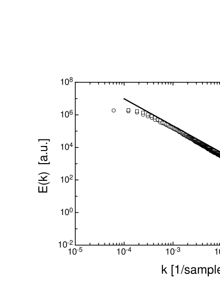
Figure 1: The wave number spectra $E(k)$ of the original data (circles) and the smoothed data set (squares). The wave number $k$ is given in units of samples. The straight line indicates scaling behaviour according to K41: $E(k)\propto k^{-5/3}$.

We therefore applied a digital low pass filter to the data multiplying the Fourier coefficients with the spectral filter function

$$\phi(k)=\frac{1}{1+(k/k_{0})^{4}}.$$ (23)

The cutoff wave number was chosen to be $k_{0}=0.2$, according to the observed transition to white noise for wave numbers $k>0.2$ (see fig. 1 which also displays the power spectrum of the filtered data set). Details on the method can be found in [23].

A digital filter is of course a serious manipulation of the data and it is by no means obvious that the smoothed data represent the ”real” velocity signal in a better approximation than the original data set. Therefore we compared the various results obtained from the original and the smoothed data. In both cases we used $\Delta=5$ for the estimation of the energy dissipation rate. It is found that for both cases the coefficients ${\mathbf{D}}^{(k)}$ show the same functional dependencies on their arguments $u$, $x$ and $r$. Thus the coefficients calculated from the original and smoothed data set, respectively, are identical up to constant factor [20]. For the purpose of the analysis presented in this paper, these effects are of no importance. We therefore restrict the discussion to the results obtained from the smoothed signal. For the filtered data set, the mean energy dissipation rate $\bar{\epsilon}$ is $0.52m^{2}/s^{3}$.

5 Experimental results

Let us start with the $u$–component of the driftvector. To this end, we have to calculate the conditional moment

$$M^{(1)}_{u}(u,x,r,\Delta r)\;=\;\frac{r}{\Delta r}\left<\,u^{\prime}(r-\Delta r)-u(r)\,|\,u(r),x(r)\,\right>$$ (24)

for various values of $u$, $x$, $r$ and $\Delta r$ and try to extrapolate it towards $\Delta r=0$ according to equation (9). Figure 2 shows the coefficient $M^{(1)}_{u}$ at scale $r=L/2$ for $u=+\sigma_{\infty}$ and $x=+1$ as a function of $\Delta r$. Over the whole range of (differences of) scales $0<\Delta r\leq 2\lambda$, the dependence of $M^{(1)}_{u}$ on $\Delta r$ can in good approximation be described by a polynomial of degree two in $\Delta r$ (see [16, 17]), thus allowing for an extrapolation towards $\Delta r=0$.

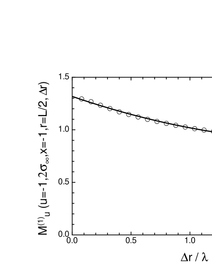
Figure 2: The coefficient $M^{(1)}_{u}(u,x,r,\Delta r)$ at scale $r=L/2$ as a function of $\Delta r$ for $u=+\sigma_{\infty}$ and $x=+1$ (circles). The data can be described and extrapolated by a polynomial of degree two in $\Delta r$ (line).

Figure 3(a) shows the result of the extrapolation for $D^{(1)}_{u}(u,x,r)$ at scale $r=L/2$ for various values of $x$ as a function of the velocity increment $u$. The $u$–component of the drift vector shows a linear dependence on the velocity increment and only weak variations for different values of $x$. To a first order approximation, the dependence of $D^{(1)}_{u}$ on $x$ can thus be neglected and we obtain:

$$D^{(1)}_{u}(u,x,r)\approx D^{(1)}_{u}(u,r)=-\tilde{\gamma}(r)u.$$ (25)

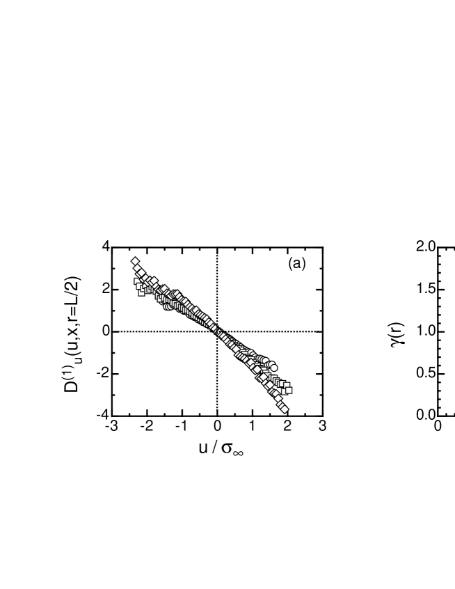
Figure 3: (a): The $u$–component $D^{(1)}_{u}(u,x,r)$ of the drift vector at scale $r=L/2$ as a function of the velocity increment $u$ for $x=-1$ (circles), $x=0$ (squares) and $x=+1$ (diamonds).
(b): The slope $\tilde{\gamma}(r)$ of $D^{(1)}_{u}(u,r)$ as a function of the scale $r$ (circles). $\tilde{\gamma}(r)$ turns out to be identical with the slope $\gamma(r)$ of the one dimensional drift coefficient (line).

The slope $\tilde{\gamma}(r)$, which for a given scale $r$ is obtained by averaging the results of the fits (25) for different $x$, has a value of $1.1$ at the scale $r=L/2$. By performing this procedure at several scales $r$ we are able to specify the scale dependence of $\tilde{\gamma}(r)$, see fig. 3(b). It turns out that the function $\tilde{\gamma}(r)$ is identical with the slope $\gamma(r)$ of the drift coefficient of the one dimensional Fokker–Planck equation (15) for $p(u,r)$.

The finding that $\tilde{\gamma}(r)$ is identical with the one dimensional coefficient $\gamma(r)$ may be surprising at first sight, but is a direct consequence of the fact that $D^{(1)}_{u}$ does (approximately) not depend on $x$. This can be seen by considering the Fokker–Planck equation (8) for the joint pdf $p(u,x,r)$:

$$-r\frac{\partial}{\partial r}p(u,x,r) = -\frac{\partial}{\partial u}\left(D^{(1)}_{u}p\right)-\frac{\partial}{\partial x}\left(D^{(1)}_{x}p\right)$$ (26)

$$+\frac{\partial^{2}}{\partial u^{2}}\left(D^{(2)}_{uu}p\right)+\frac{\partial^{2}}{\partial x^{2}}\left(D^{(2)}_{xx}p\right)+2\frac{\partial^{2}}{\partial u\partial x}\left(D^{(2)}_{ux}p\right)$$

From the two dimensional equation (26) the equation for $p(u,r)$ can be derived by integrating with respect to $x$: $p(u,r)=\int p(u,x,r)dx$. Assuming that the product $D^{(k)}_{i}(u,x,r)p(u,x,r)$ vanishes for $x\rightarrow\pm\infty$ one obtains:

$$-r\frac{\partial}{\partial r}p(u,r) = -r\frac{\partial}{\partial r}\int p(u,x,r)dx$$ (27)

$$= -\frac{\partial}{\partial u}\left(D^{(1)}_{u}(u,r)\int p(u,x,r)dx\right)$$

$$+\frac{\partial^{2}}{\partial u^{2}}\left(\int D^{(2)}_{uu}(u,x,r)p(u,x,r)dx\right)$$

$$= -\frac{\partial}{\partial u}\left(D^{(1)}(u,r)p(u,r)\right)$$

$$+\frac{\partial^{2}}{\partial u^{2}}\underbrace{\int D^{(2)}_{uu}(u,x,r)p(x,r|u,r)dx}_{D^{(2)}(u,r)}\,p(u,r).$$

The result of this calculation is a one dimensional Fokker–Planck equation for $p(u,r)$ with a drift coefficient $D^{(1)}(u,r)$ that is identical to its two dimensional counterpart $D^{(1)}_{u}(u,r)$.

The second order coefficient $D^{(2)}_{uu}(u,x,r)$ can be estimated by an extrapolation of the conditional second order moments

$$M^{(2)}_{uu}(u,x,r,\Delta r)=\frac{r}{2\Delta r}\left<\left(u^{\prime}(r-\Delta r)-u(r)\right)^{2}|u(r),x(r)\right>$$ (28)

towards $\Delta r\rightarrow 0$ in the same way as described above for the first order coefficient $D^{(1)}_{u}$. As can be seen in figure 4, the coefficient $D^{(2)}_{uu}$ does not depend on the velocity increment $u$ and shows an exponential dependence on $x$:

$$D^{(2)}_{uu}(u,x,r)=D^{(2)}_{uu}(x,r)=a_{0}(r)\exp\left(a_{1}(r)x\right)$$ (29)

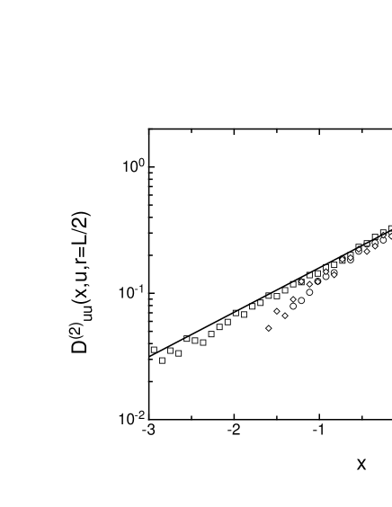
Figure 4: The $uu$–component $D^{(2)}_{uu}(u,x,r)$ of the diffusion matrix at scale $r=L/2$ as a function of $x$ for $u=-\sigma_{\infty}$ (circles), $u=0$ (squares) and $u=+\sigma_{\infty}$ (diamonds). The coefficient does not depend on $u$ and can be described by an exponential in $x$ (the straight line represents a fit to the data for $u=0$ according to eq. (29)).

The coefficients $a_{0}$ and $a_{1}$ defined in eq. (29) show simple dependencies on the scale $r$ (see figure 5): $a_{0}$ is a linear function of $r$, while $a_{1}$ is constant:

$$a_{0}(r) \approx 0.02\left(\frac{r}{\lambda}-1\right),$$

$$a_{1} \approx 0.9.$$ (30)

Note that the linear dependence of $a_{0}$ on the scale $r$ as specified in eq. (30) leads to negative values for $D^{(2)}_{uu}$ on scales smaller than the Taylor microscale $\lambda$. This is in contradiction to the definitions (9) and (10) of the diffusion matrix since, according to those definitions, the diagonal–elements of ${\mathbf{D}}^{(2)}$ are positive quantities. The finding of negative values for $D^{(2)}_{uu}$ on scales smaller than $\lambda$ indicates that, similar to the one dimensional case, the Markovian property cannot be fulfilled for such small scales.

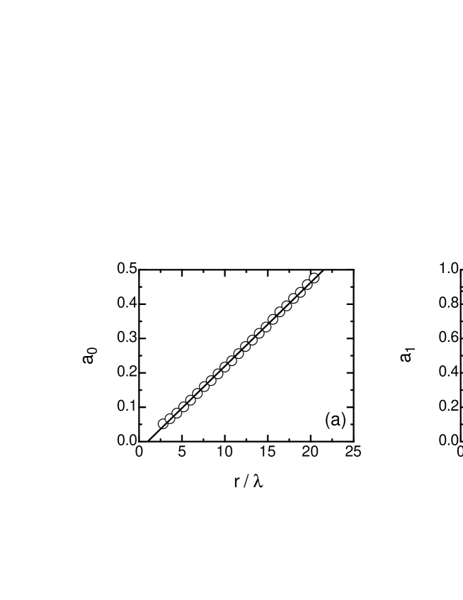
Figure 5: The coefficients $a_{0}$ (a) and $a_{1}$ (b) defined in eq. (4) as functions of the scale $r$. $a_{0}$ is a linear function of $r$, $a_{1}$ is approximately constant (straight lines).

The fact that $D^{(2)}_{uu}(u,x,r)$ does not depend on $u$ is a very interesting result since it states that the effect of intermittency is caused by the stochastic nature of the energy dissipation rate. This can be seen by considering equation (27) for the (hypothetical) K41–case that $\epsilon_{r}$ is not a stochastic variable but constant. In this case the conditional pdf $p(x,r|u,r)$ in equation (27) is formally given by $p(x,r|u,r)=p(x,r)=\delta(x-1)$ and the one dimensional coefficient $D^{(2)}$ can easily be calculated: $D^{(2)}=\int D^{(2)}_{uu}(x,r)p(x,r|u,r)dx=D^{(2)}_{uu}(x=1,r)=D^{(2)}(r)$. With a diffusion coefficient that does not depend on $u$ the resulting Fokker–Planck equation (27) for $p(u,r|\epsilon_{r}=const)$ can be shown to be solved by a Gaussian distribution [15]. The effect of intermittecy can thus be clearly traced back to the statistics of $\epsilon_{r}$. This result is in full agreement with the results for the conditional pdf $p(u(r)|\epsilon_{r})$ presented in [7, 8].

Before proceeding with the $x$–components of drift vector and diffusion matrix, let us draw attention to the mixed term $D^{(2)}_{ux}$ of the diffusion matrix. This term can be estimated by extrapolating the conditional moments

$$M^{(2)}_{ux}=\frac{r}{2\Delta r}\left<\,\left(u^{\prime}(r-\Delta r)-u(r)\right)\left(x^{\prime}(r-\Delta r)-x(r)\right)\,|\,u(r),x(r)\,\right>$$ (31)

towards $\Delta r\rightarrow 0$. Figure 6(a) shows the coefficient $M^{(2)}_{ux}$ at scale $r=L/2$ for exemplarily chosen values of $u$ and $x$ as a function of $\Delta r$. The coefficient exhibits large variations with $\Delta r$ and its absolute value shows a strong decrease as $\Delta r$ goes to zero. This may be taken as a first hint that $M^{(2)}_{ux}$ vanishes in the limit $\Delta r\rightarrow 0$.

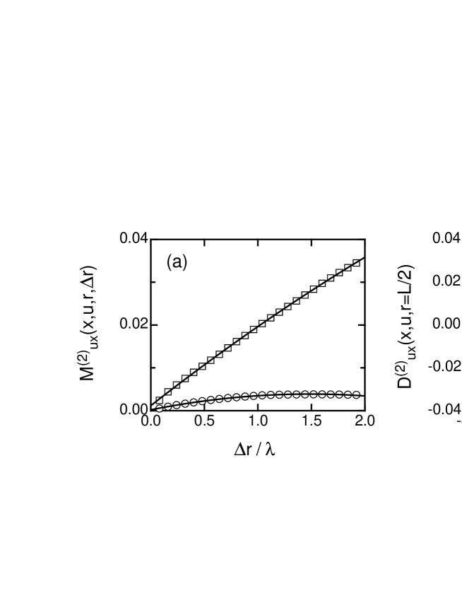
Figure 6: (a): The conditional moment $M^{(2)}_{ux}(u,x,r,\Delta r)$ at scale $r=L/2$ as a function of $\Delta r$ for $u=-0.6\sigma_{\infty},x=-3$ (squares) and $u=+0.6\sigma_{\infty},x=+1$ (circles). The data can be extrapolated by polynomials of degree two (lines).
(b): The extrapolated coefficient $D^{(2)}_{ux}(u,x,r)$ at scale $r=L/2$ as a function of $x$ for $u=-\sigma_{\infty}$ (squares), $u=0$ (circels) and $u=+\sigma_{\infty}$ (diamonds).

When the extrapolation towards $\Delta r\rightarrow 0$ is performed by fitting polynomials of degree two to the data in the interval $0<\Delta r\leq 2\lambda$ (see fig. 6a), we obtain values for $D^{(2)}_{ux}$ which are small compared to the corresponding values of $M^{(2)}_{ux}$ at finite $\Delta r$. Furthermore, the coefficient $D^{(2)}_{ux}$ shows fluctuations which are of the order of magnitude of the values themselves (see fig. 6b). We take this as evidence that the mixed coefficient $D^{(2)}_{ux}$ vanishes.

Given that the off–diagonal element $D^{(2)}_{ux}$ of the diffusion matrix vanishes, the functions ${\mathbf{g}}(u,x,r)$ in the Langevin–equation (11) can easily be calculated according to equation (12). In Itô’s formalism, ${\mathbf{g}}$ is then simply given by:

$$g_{uu}=\sqrt{\frac{1}{r}D^{(2)}_{uu}},\qquad g_{ux}=g_{xu}=0,\qquad g_{xx}=\sqrt{\frac{1}{r}D^{(2)}_{xx}}.$$ (32)

With the results obtained so far the Langevin–equation (11) takes the form:

$$-\frac{\partial}{\partial r}u(r) \;=\; \frac{\gamma(r)}{r}u\,+\,\sqrt{\frac{a_{0}(r)}{r}\exp\left(a_{1}x(r)\right)}\,\Gamma_{u}(r),$$

$$-\frac{\partial}{\partial r}x(r) \;=\; \frac{1}{r}D^{(1)}_{x}(u,x,r)\,+\,\sqrt{\frac{1}{r}D^{(2)}_{xx}(u,x,r)}\,\Gamma_{x}(r).$$ (33)

Even though the formulation (33) of the twodimensional Langevin–equation is yet incomplete, it can already be used to extract the $u$–component $\Gamma_{u}(r)$ of the stochastic force from measured realizations of $u(r)$, $\frac{\partial}{\partial r}u(r)$ and $x(r)$. These calculations are faciliated by the fact that the diffusion coefficient $D^{(2)}_{uu}$ does not depend on the velocity increment $u$. It is therefore not necessary to distinguish between the various definitions of stochastic calculus (Itô and Stratonovich, respectively), and a simple Euler–scheme can be applied to calculate $\Gamma_{u}(r)$ (for details on the numerical scheme see, for example, [13]).

The stoachstic process governing the $r$–evolution of the stochastic variable ${\mathbf{q}}(r)$ is Markovian, if the stochastic force ${\mathbf{\Gamma}}$ is $\delta$–correlated. However, as can be seen in figure 7, the autocorrelation function $R_{\Gamma}(\Delta r)$ of the stochastic force $\Gamma_{u}(r)$ exhibits nonzero values up to $\Delta r\approx\lambda$. This clearly indicates that the Markovian properties are fulfilled for scales $r$ (and differences of scales $\Delta r$) larger than the Taylor microscale $\lambda$ only. Again, we recall that this result is in agreement with the one dimensional analysis of the velocity increment (see [11]).

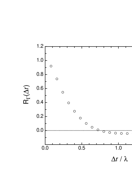
Figure 7: The autocorrelation function $R_{\Gamma}(\Delta r)$ of the $u$–component $\Gamma_{u}(r)$ of the stochastic force ${\mathbf{\Gamma}}(r)$ (open circles). $R_{\Gamma}(\Delta r)$ exhibits finite values up to scales $\Delta r\approx\lambda$.

To complete the description of the turbulent cascade by the Markov analysis, we still have to determine the coefficients $D^{(1)}_{x}$ and $D^{(2)}_{xx}$ by extrapolating the conditional moments $M^{(1)}_{x}(u,x,r,\Delta r)$ and $M^{(2)}_{xx}(u,x,r,\Delta r)$, respectively. As shown in fig. 8(a) for exemplarily chosen values of $u$, $x$ and $r$, the first order coefficient $M^{(1)}_{x}$ can be described by a polynomial of degree two in $\Delta r$ over the whole range of scales $0<\Delta r\leq 2\lambda$, which again allows for an extrapolation towards $\Delta r=0$.

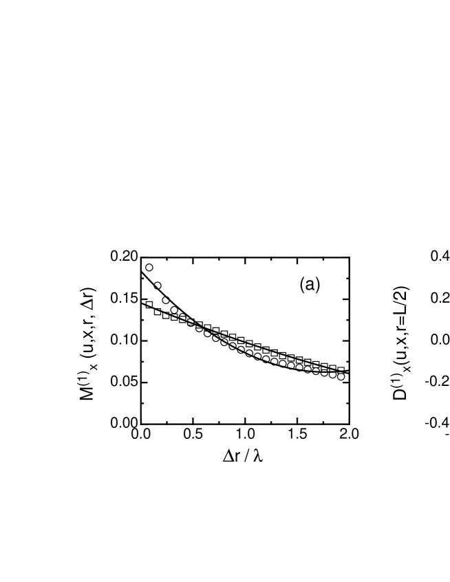
Figure 8: (a): The conditional moment $M^{(1)}_{x}(u,x,r,\Delta r)$ at scale $r=L/2$ as a function of $\Delta r$ for $u=-0.6\sigma_{\infty},x=+1$ (circles) and $u=+0,6\sigma_{\infty},x=+1$ (squares). The data can be extrapolated by polynomials of degree two (lines).
(b): The extrapolated coefficient $D^{(1)}_{x}(u,x,r)$ at scale $r=L/2$ as a function of $x$ for $u=-\sigma_{\infty}$ (squares), $u=0$ (circles) and $u=+\sigma_{\infty}$ (diamonds).

The coefficient $D^{(1)}_{x}$ turns out to be a linear function of the logarithmic energy dissipation rate $x(r)$ and does not depend on the velocity increment $u$, see fig. 8(b):

$$D^{(1)}_{x}(u,x,r)=D^{(1)}_{x}(x,r)=F(r)+G(r)x$$ (34)

Since the coefficient $D^{(1)}_{x}$ does not depend on $u$, it has to be identical with the coefficient $D^{(1)}$ of the one dimensional Fokker–Planck equation (17) for $p(x,r)$. This follows from an analogous consideration leading to equation (27).

Plotting $F$ and $G$ as functions of the linear scale $r$, we find that their scale dependence is best described by (see fig. 9):

$$F(r) \approx 0.05-0.04\ln\left(\frac{r}{\lambda}\right)$$

$$G(r) \approx 0.03\left(\frac{r}{\lambda}\right)^{0.57}.$$ (35)

Note that these parametrizations differ from those given for the one dimensional coefficients in equation (19). However, the discrepancy between the results given in (35) and (19) must not be taken too serious. In [13] $F$ and $G$ were plotted in terms of the invers logarithmic length scale $l=\ln\left(L/r\right)$, which may suggest a different functional dependence of those coefficients on the scale than it is found here. Furthermore, a data set at $R_{\lambda}=341$ was used, whereas for the data set used here the Taylor–Reynolds number is $463$. In addition, as mentioned above, numerical values such as those for $F(r)$ and $G(r)$ strongly depend on the method chosen to estimate the derivative $\frac{\partial v}{\partial x}$ (see chapter 4).

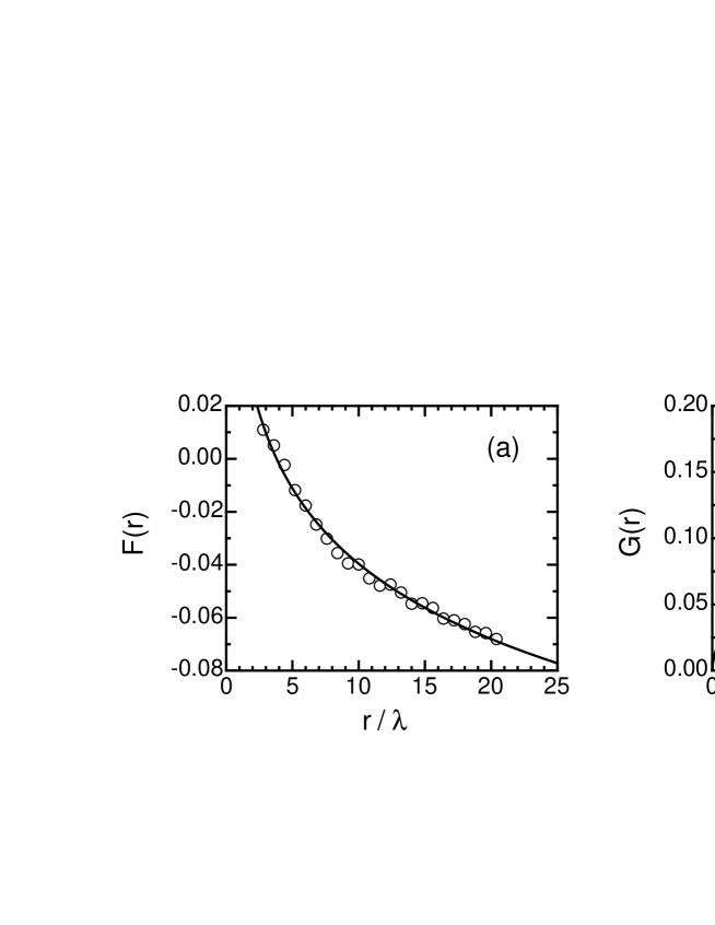
Figure 9: (a): The constant term $F(r)$ of the drift coefficient $D^{(1)}_{x}$ as a function of the scale $r$. The full line indicates a fit according to eq. (35).
(b): The slope $G(r)$ of $D^{(1)}_{x}$ as a function of $r$. Full line: fit according to eq. (35); dotted line: fit according to eq. (19).

The last coefficient which remains to be calculated is the $xx$–component of the diffusion matrix. Unfortunately, the estimation of $D^{(2)}_{xx}(u,x,r)$ from the conditional moment

$$M^{(2)}_{xx}(u,x,r,\Delta r)=\frac{r}{2\Delta r}\left<\left(x^{\prime}(r-\Delta r)-x(r)\right)^{2}|u(r),x(r)\right>$$ (36)

yields several difficulties. When plotted as a function of $\Delta r$, the conditional moment $M^{(2)}_{xx}$ shows a strong decrease as $\Delta r$ goes to zero (see fig. 10): The extrapolated values of $D^{(2)}_{xx}$ are small compared to the values of $M^{(2)}_{xx}$ for finite values of $\Delta r$.

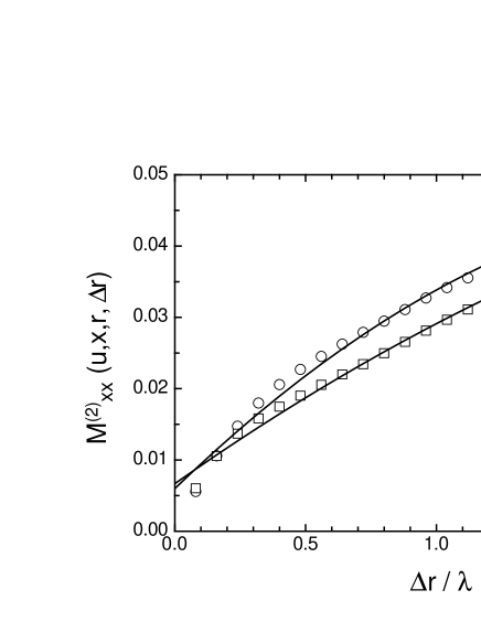
Figure 10: The conditional moment $M^{(2)}_{xx}(u,x,r,\Delta r)$ at scale $r=L/2$ as a function of $\Delta r$ for $u=-0.6\sigma_{\infty},x=+1$ (circles) and $u=+0,6\sigma_{\infty},x=+1$ (squares). The data were extrapolated by polynomials of degree two (lines).

Accordingly, the coefficient $D^{(2)}_{xx}$ at scale $r=L/2$ does not exhibit systematic dependencies on its arguments $x$ or $u$, see fig. 11(a). Although the values seem to decrease for large values of $|x|$ with a maximum at $x\approx-2$, the considerable scatter of the data also allows to assume a constant value for $D^{(2)}_{xx}$. A different result is obtained for smaller scales, as shown exemplarily for $r=4\lambda$ in fig. 11(b). In this case the coefficient $D^{(2)}_{xx}$ clearly exhibits a dependence on the energy dissipation rate $x$ as well as a dependence on the velocity increment $u$. However, from the data presented in fig. 11(b) it is still impossible to decide how the dependence of $D^{(2)}_{xx}$ is to be parametrized; the data can be fitted with several functions (Gaussian as well as Lorentzian distributions, for example) with almost equal accuracy. The question of whether one of these functions is to be preferred requires further detailled experimental as well as theoretical investigations and is the subject of an ongoing study.

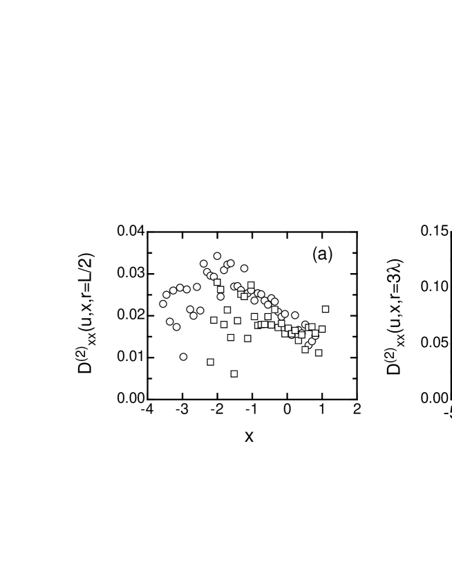
Figure 11: The $xx$–component $D^{(2)}_{xx}(u,x,r)$ of the diffusion matrix as a function of the logarithmic dissipation rate $x$. (a): At scale $r=L/2$ for $u=0$ (circles) and $u=+\sigma_{\infty}$ (squares). (b): At scale $r=3\lambda$ for $u=0$ (circles) and $u=\frac{1}{4}\sigma_{\infty}$ (squares).

6 Conclusion and Comments

Although further investigations will be necessary to complete the two dimensional Markov analysis of the turbulent cascade, the results obtained so far already allow for several interesting statements on the joint statistical properties of the longitudinal velocity increment and the averaged energy dissipation rate.

A particularly remarkable result is obtained for the $u$–component $D^{(2)}_{uu}$ of the diffusion matrix, which is found not to depend on the velocity increment. This means that if the averaged energy dissipation rate $\epsilon_{r}$ was not a stochastic variable but constant, the pdf of $u(r)$ would reduce to a rather simple Gaussian distribution. The effect of small scale intermittency can thus clearly be traced back to the stochastic nature of $\epsilon_{r}$.

So far, our results are in accordance with earlier experimental investigations [7, 8] as well as with the assumptions underlying Kolmogorov’s models. Significant new information, however, are found for the $u$–component of the drift vector. We found that $D^{(1)}_{u}(u,x,r)$ does not depend on the energy dissipation rate, in a first order approximation. This means that this coefficient is identical with the drift term of the one dimensional Fokker–Planck equation for $p(u,r)$, i.e. it reveals a linear dependence on $u$ with a slope $\gamma(r)$ given by eq. (16). With respect to the works [9, 10, 24, 25] it remains open to explain why $\gamma$ deviates from the value $1/3$.

A further new important result is that the drift coefficient $D^{(1)}_{x}$ does not depend on the velocity increment $u$ and is a linear function of the logarithmic energy dissipation rate $x$ as specified by eq. (34). One thus obtains a system of two stochastic differential equations for the evolution of $u$ and $x$ in $r$ which are linked only via their stochastic terms while the deterministic parts of the equations for $u$ and $x$ do not depend on the other variable.

To summarize, the Langevin–equation for the two dimensional stochastic variable ${\mathbf{q}}(r)=\left(\,u(r),x(r)\,\right)$ reads:

$$-\frac{\partial}{\partial r}\,u(r)\; = \;-\frac{1}{r}\,\gamma(r)\,u(r)\;+\;m\,\exp\left(\frac{a_{1}}{2}x(r)\right)\;\Gamma_{u}(r),$$

$$-\frac{\partial}{\partial r}\,x(r)\; = \;+\frac{1}{r}\,G(r)\,x(r)\;+\;\frac{1}{r}\,F(r)\;+\;\sqrt{\,\frac{1}{r}\,D^{(2)}_{xx}(u,x,r)\,}\;\Gamma_{x}(r)\,.$$ (37)

According to eq. (30), the coefficient $m=\sqrt{\frac{a_{0}(r)}{r}}$ in the stochastic part of the equation for $u(r)$ is approximately constant in $r$ (see also fig. 5). Note also that, when rewritten in terms of $\epsilon_{r}$, the stochastic term in the equation for $u(r)$ exhibits a simple power–law dependence on the energy dissipation rate: $\exp\left(a_{1}x/2\right)=\left(\epsilon_{r}/\bar{\epsilon}\right)^{a_{1}/2}\approx\sqrt{\epsilon_{r}/\bar{\epsilon}}$ (see fig. 5b).

It is interesting to compare the two dimensional equation (37) with the one dimensional Langevin–equations for $u(r)$ and $x(r)$ discussed in section 3. Those equations read:

$$-\frac{\partial}{\partial r}\,u(r)\; = \;-\frac{1}{r}\,\gamma(r)\,u(r)\;+\;\sqrt{\,\frac{1}{r}\,\left(\,\alpha(r)-\delta(r)u+\beta(r)u^{2}\,\right)\,}\;\Gamma(r)\,,$$

$$-\frac{\partial}{\partial r}\,x(r)\; = \;+\frac{1}{r}\,G(r)\,x(r)\;+\;\frac{1}{r}\,F(r)\;+\;\sqrt{\,\frac{1}{r}\,D(r)\,}\;\Gamma(r)\,.$$ (38)

Compared to the one dimensional Langevin–equation, the stochastic part of the equation for $u(r)$ is considerably simpler for the two dimensional process. Note also that the resulting equation for the evolution of $u(r)$ in two dimensions is symmetric in $u\rightarrow-u$: if $x$ was constant, the solutions of eq. (37) would be symmetric in $u$, thus leading to vanishing odd order moments. Asymmetries of the velocity increment, which are of importance in Kolmogorov’s four–fifths law, can thus clearly be attributed to the influence of the energy cascade.

While the equation for the velocity increment simplifies considerably in the two dimensional formulation, the diffusion coefficient $D^{(2)}_{xx}(u,x,r)$ seems to exhibit a more complex dependence on its arguments (see fig. 11) than the one dimensional coefficient $D(r)$. Whether the dependence of $D^{(2)}_{xx}$ on $x$ is in fact given by the rather complex form indicated in fig. 11(b) is yet an open problem which requires further discussions of the experiemental uncertainties. However, it is also conceivable that an even more complete characterization of the turbulent cascade has to include the transversal velocity increment as well. Such a three–dimensional analysis might lead to further simplifications of the diffusion terms.

Nevertheless, the results obtained so far give reason to believe that the mathematical framework of stochastic Markovian processes is a suitable tool for experimental investigations concerning the joint statistical properties of velocity increments and the energy dissipation rate in fully developed turbulence. As it is known that the Fokker–Planck equation holds for the conditional pdf as well, the knowledge of this equation also provides all information about any N–scale joint pdf of $x$ and $u$, see equations 7 and 8. Thus any general moment of $u(r)^{\alpha}x(r^{\prime})^{\beta}$ is known. In this way the phenomenological Fokker–Planck equation derived from the data provides a closed description for all moments on all scales.

References

- [1] K.R. Sreenivasan, R.R. Antonia, Ann. Rev. Fluid Mech., 29 435 (1997); U. Frisch, Turbulence. Cambridge University Press, Cambridge 1996; S.B. Pope, Turbulent Flows. Cambridge University Press, Cambridge, 2000.
- [2] A.N. Kolmogorov, The local structure of turbulence in an incompressible viscous fluid for very high Reynolds number. Dokl. Akad. Nauk. SSSR 30, 301 (1941).
- [3] A.N. Kolmogorov, A refinement of previous hypotheses concerning the local structure of turbulence in a viscous incompressible fluid at high Reynolds number. J. Fluid Mech 13, 82 (1962).
- [4] L.F. Richardson, Weather prediction by numerical process. Cambridge University Press, Cambridge, 1922.
- [5] L.D. Landau & E.M. Lifschitz, Fluid Mechanics, 2nd edition, Pergamon Press, Oxford, 1987.
- [6] B. Castaing, Y. Gagne & E.J. Hopfinger, Velocity probability density functions of high Reynolds number turbulence. Physica D 46, 177 (1990).
- [7] Y. Gagne, M. Marchand & B. Castaing, Conditional velocity pdf in 3–D turbulence. J. Phys. II France 4, 1 (1994).
- [8] A. Naert et al., Conditional statistics of velocity fluctuations in turbulence. Physica D 113(1), 73 (1998).
- [9] R. Friedrich & J. Peinke, Description of a turbulent cascade by a Fokker–Planck equation. Phys. Rev. Lett. 78(5), 863 (1997).
- [10] R. Friedrich & J. Peinke, Statistical properties of a turbulent cascade. Physica D 102, 147 (1997).
- [11] Ch. Renner, J. Peinke & R. Friedrich, Experimental Indications for Markov properties of small–scale turbulence. J. Fluid Mech, 433, 383 (2001).
- [12] A. Naert, R. Friedrich & J. Peinke, Fokker–Planck equation for the energy cascade in turbulence. Phys. Rev. E 56(6), 6719 (1997).
- [13] P. Marq & A. Naert, A Langevin equation for the energy cascade in fully developed turbulence. Physica D 124(4), 368 (1998).
- [14] J. Cleve & M. Greiner, The Markovian metamorphosis of a simple turbulent cascade model. Phys. Lett. A 273, 104-108 (2000).
- [15] H. Risken, The Fokker-Planck equation, Springer-Verlag Berlin, 1984.
- [16] M. Ragwitz & H. Kantz, Indispensable Finite Time Corrections for Fokker–Planck Equations from Time Series Data. Phys. Rev. Lett. 87, 254501 (2001).
- [17] R. Friedrich, Ch. Renner, M. Siefert & J. Peinke, Comment on ”Indispensable Finite Time Corrections for Fokker–Planck Equations from Time Series Data”. Phys. Rev. Lett. 87(14), 149401-1 (2002).
- [18] S. Siegert, R. Friedrich & J. Peinke, Analysis of data sets of stochastic systems. Phys. Lett. A 243(5-6), 275 (1998).
- [19] Ch. Renner, J. Peinke, R. Friedrich, O. Chanal & B. Chabaud, On the universality of small–scale turbulence. Phys. Rev. Lett. 89(12), 124502 (2002).
- [20] Ch. Renner, Markowanalysen stochastisch fluktuierender Zeitserien, PhD–thesis, Oldenburg, 2002
- [21] O. Chanal, Vers les echelles dissipatives dans und jet d’Helium gazeux a basse temperature. PhD–thesis, Grenoble, 1998.
- [22] O. Chanal et al., Intermittency in a turbulent low temperature gaseous helium jet. Eur. Phys. J. B 17(2), 309 (2000).
- [23] W.H. Press et al. Numerical Recipes in C. The Art of Scientific Computing. Cambridge University Press, Cambridge 1986.
- [24] V. Yakhot, Probability density and scaling exponents of the moments of longitudinal velocity difference in strong turbulence. Phys. Rev. E 57(2), 1737 (1998).
- [25] J. Davoudi & M.R. Tabar, Theoretical model of the Kramers–Moyal description of turbulence cascades. Phys. Rev. Lett. 82, 1680 (1999).
- [26] N. Mordant, J.–F. Pinton & F. Chilla, Characterization of turbulence in a closed flow. J. Phys. II 7 (11), 1729 (1997).