Compressibility effects on the scalar mixing in reacting homogeneous turbulence

Abstract

The compressibility and heat of reaction influence on the scalar mixing in decaying isotropic turbulence and homogeneous shear flow are examined via data generated by direct numerical simulations (DNS). The reaction is modeled as one-step, exothermic, irreversible and Arrhenius type. For the shear flow simulations, the scalar dissipation rate, as well as the time scale ratio of mechanical to scalar dissipation, are affected by compressibility and reaction. This effect is explained by considering the transport equation for the normalized mixture fraction gradient variance and the relative orientation between the mixture fraction gradient and the eigenvectors of the solenoidal strain rate tensor.

1 Introduction

Recent studies of scalar mixing in incompressible turbulence (e.g. Overholt & Pope 1996; Jaberi et al. 1996; Slessor, Bond & Dimotakis 1998; Livescu, Jaberi & Madnia 2000) have enhanced our understanding of the mixing mechanism, the behavior of the scalar PDF and the evolution of scalar moments. However, fundamental studies of scalar mixing in compressible turbulence are scarce. Blaisdell, Mansour & Reynolds (1994) show that the dilatational velocity has negligible contribution to the scalar flux in homogeneous turbulence. It is not clear, however, how the compressibility affects the scalar moments or the scalar dissipation. A better understanding of the compressibility effects is important in the analysis of the combustion processes. The main objective of this work is to study the influence of compressibility and heat release on the evolution of the scalar dissipation rate in homogeneous turbulence.

2 Numerical methodology and DNS parameters

In order to assess the influence of compressibility on the mixing process, direct numerical simulations (DNS) of decaying isotropic and homogeneous sheared turbulence are performed under reacting (heat - releasing) and nonreacting conditions. In the nonreacting cases a passive scalar is simulated along with the turbulent field. The compressible form of continuity, momentum, energy and species mass fractions transport equations are solved using the spectral collocation method. In the reacting cases, the chemical reaction is modeled by a one-step irreversible Arrhenius-type reaction. In order to assess the influence of heat of reaction on the mixing process, the statistics pertaining to the mixture fraction $Z$ are extracted from the two reacting scalar fields and compared to those obtained for a passive scalar in the nonreacting cases. The viscosity varies with the temperature according with a power law and $Le=1$ in all cases.

For the shear flow simulations, the velocity fluctuations are initialized as a random solenoidal, three-dimensional field with Gaussian spectral density function (with the peak at $k_{0v}=10$) and unity rms. The initial pressure fluctuations are evaluated from a Poisson equation (except for the high Mach number case for which they are set to zero). For the decaying isotropic simulations the initialization proposed by Ristorcelli & Blaisdell (1997) is employed. The variables are then allowed to decay until they develop realistic turbulence fluctuations before the scalars are initialized. This corresponds to time $t=0$ on all figures. The value of the Reynolds number at $t=0$ is $Re_{\lambda_{0}}=50$. The simulations are stopped at $t/\tau_{t}=14.4$ such that the scalar variance becomes two orders of magnitude less than the initial value. For the shear flow cases $Re_{\lambda_{0}}=21$ initially, and increases to values between $93-110$ in the direction of the mean velocity at the end of the simulations. The shear flow simulations are stopped between $18<St<20$, such that the integral scales remain small compared to box size and the Kolmogorov microscale is larger than the grid size. This corresponds to $t/\tau_{t}$ in the range $10.4$ to $11.5$.

The scalar fields are initialized as “random blobs”, with double-delta PDFs (Overholt & Pope, 1996). The initial length-scale of the scalar field is controlled by changing the location, $k_{0s}$, of the peak of the Gaussian spectrum used to generate the scalar field. The variables are time advanced in physical space using a second order accurate Adams-Bashforth scheme. The code developed for this work is based on a fully parallel algorithm and uses the standard Message Passing Interface (MPI).

In order to examine the compressibility effects on the scalar mixing, cases with different initial value of the turbulent Mach number, $M_{t_{0}}$, are considered. The heat release effects are investigated by varying the values of the heat release parameter, $Ce$, computational Damk$\ddot{\rm{o}}$hler number, $Da$, and the initial lengthscale of the scalar field. All reacting cases have the value of the Zeldovich number, $Ze=8$. Table 1 summarizes the cases considered for this study. The isotropic turbulence cases are labeled with $i$ and the shear flow cases with $s$. For the shear flow cases the value of the initial nondimensional mean shear rate, $S_{0}^{*}=\frac{S(2K)}{\epsilon}$, where $K$ is the turbulent kinetic energy and $\epsilon$ is the viscous dissipation, is in the range dominated by nonlinear effects. $S=\partial\tilde{u_{1}}/\partial x_{2}$ ($\tilde{\mbox{ }}$ is the Favre average) is the mean shear rate.

Table 1: Parameters for the DNS cases.

Case $\#$	$M_{t_{0}}$	$S_{0}^{*}$	$Da$	$Ce$	$k_{0_{s}}$
$i1$	0.2	0	0	0	4
$i2$	0.35	0	0	0	4
$i3$	0.5	0	0	0	4
$s1$	0.1	7.24	0	0	4
$s2$	0.2	7.24	0	0	4
$s3$	0.3	7.24	0	0	4
$s4$	0.4	7.24	0	0	4
$s5$	0.6	7.24	0	0	4
$s6$	0.3	7.24	1100	1.44	4
$s7$	0.3	7.24	1100	2.16	4
$s8$	0.3	7.24	1750	1.44	4
$s9$	0.3	7.24	1100	1.44	10

The reaction parameters chosen for the cases considered mimic the combustion of a typical hydrocarbon in air at low to moderate values of Reynolds number. For all reacting cases presented most of the reaction occurs between $2<St<8$ and the reaction rate peaks between $4<St<6$.

3 Results

In the absence of a mean scalar gradient, the transport equation for the mixture fraction variance, $\widetilde{Z^{\prime\prime}Z^{\prime\prime}}$, does not have a production term and $\widetilde{Z^{\prime\prime}Z^{\prime\prime}}$ decays continuously. Furthermore, if the transport equation for the mixture fraction variance is normalized by $\widetilde{Z^{\prime\prime}Z^{\prime\prime}}$ then the right hand side is proportional to the mixture fraction dissipation rate, $\epsilon_{Z}=\frac{1}{\widetilde{Z^{\prime\prime}Z^{\prime\prime}}}<\frac{\mu}{ReSc}\nabla Z^{\prime\prime}\cdot\nabla Z^{\prime\prime}>$ which is a key quantity in the modeling of both passive and reactive turbulent scalar fields. For all cases considered $\epsilon_{Z}$ increases initially as the turbulence breaks down the non-premixed “blobs” into smaller scalar structures, then it reaches a maximum and starts to decay. For the isotropic turbulence cases our results indicate a slight dependence of $\epsilon_{Z}$ on $M_{t_{0}}$. However, for the shear flow simulations, figure 1(a) shows that the values of $\epsilon_{Z}$ decrease as $M_{t_{0}}$ increases. Since for the nonreacting cases the variation of the viscosity is small, the decrease in $\epsilon_{Z}$ with Mach number can be associated with the decrease in the normalized mixture fraction gradient variance, $\xi=<\nabla Z^{\prime\prime}\cdot\nabla Z^{\prime\prime}>/\widetilde{Z^{\prime\prime}Z^{\prime\prime}}$. This is in agreement with the results obtained for forced isotropic turbulence by Cai, O’Brien & Ladeinde (1998). In the presence of heat release, $\epsilon_{Z}$ increases its magnitude during the time when the reaction is significant (figure 1b). A further increase in the values of $\epsilon_{Z}$ is obtained by increasing $Ce$ or $Da$. However, for the reacting cases, our results indicate that the values of $\xi$ decrease due to the reaction. Therefore, the increase in $\epsilon_{Z}$ can be associated with the significant enhancement of the molecular transport properties due to the heat of reaction. By increasing the value of $k_{0_{s}}$ (case $s9$) the initial length scale of the scalar field becomes smaller, which results in higher values of $\epsilon_{Z}$ compared to other cases.

Figure 1: a) Mach number and b) heat release influence on the evolution of the mixture fraction dissipation rate.

The scalar dissipation rate is usually modeled by assuming that the ratio, $C_{Z}=\frac{2K/\epsilon}{1/\epsilon_{Z}}$, of the time scale of mechanical dissipation to that of the mixture fraction variance dissipation is constant, although there is much evidence that it does not take a universal value (Livescu, Jaberi & Madnia 2000). Figure 2 shows that for the isotropic turbulence cases $C_{Z}$ varies in time initially and seems to asymptote to a constant at long time. Similar with the results obtained for the mixture fraction dissipation rate, $C_{Z}$ is slightly affected by the change in $M_{t_{0}}$ for the cases considered. For comparison, also shown are the corresponding values of $C_{Z}$ obtained using the model of Xu, Antonia & Rajagopalan (2000). The model assumes local isotropy, and the prediction plotted in figure 2 does not take into account the intermittency of the small scales. The values of $C_{Z}$ become close to the model prediction at late times.

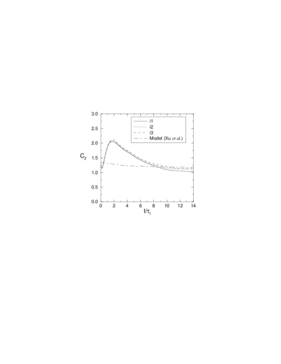
Figure 2: Time variation of $C_{Z}$ for the isotropic turbulence cases.

Both $M_{t_{0}}$ and heat of reaction influence the values of $C_{Z}$ in the shear flow simulations (figure 3). For the nonreacting cases, $C_{Z}$ decreases as $M_{t_{0}}$ increases (figure 3a). At early times this is due to an amplification of the viscous dissipation rate, $\epsilon/K$, and a decrease in $\epsilon_{Z}$. At later times $\epsilon/K$ has lower values at higher $M_{t_{0}}$, which explains the change in the slope of $C_{Z}$ observed in figure 3(a). For the reacting cases the viscous dissipation rate increases significantly during the time when reaction is important. This increase is larger than the increase in $\epsilon_{Z}$, and $C_{Z}$ becomes less than in the nonreacting case (figure 3b).

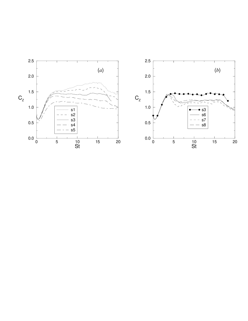
Figure 3: a) Mach number and b) heat release influence on the evolution of $C_{Z}$.

It is explained above that the normalized mixture fraction gradient, decreases at higher values of $M_{t_{0}}$ or in the presence of heat release. This behavior is further examined by considering the transport equation for the normalized variance of the mixture fraction gradient:

$$\frac{d\xi}{dt}=I+II+III+IV+V$$ (1)

where

$$I = -2<\nabla Z^{\prime\prime}\cdot\underline{\underline{S}}\cdot\nabla Z^{\prime\prime}>/\widetilde{Z^{\prime\prime}Z^{\prime\prime}}$$

$$II = -2<\nabla Z^{\prime\prime}\cdot\underline{\underline{s^{s}}}\cdot\nabla Z^{\prime\prime}>/\widetilde{Z^{\prime\prime}Z^{\prime\prime}}$$

$$III = -2<\nabla Z^{\prime\prime}\cdot\underline{\underline{s^{d}}}\cdot\nabla Z^{\prime\prime}>/\widetilde{Z^{\prime\prime}Z^{\prime\prime}}$$

$$IV = <\Delta(\nabla Z^{\prime\prime}\cdot\nabla Z^{\prime\prime})>/\widetilde{Z^{\prime\prime}Z^{\prime\prime}}$$

$$V = -\left[\frac{2\tilde{\mu}}{ReSc<\rho>}\left<\left(\nabla^{2}Z^{\prime\prime}\right)^{2}-\frac{<\nabla Z^{\prime\prime}\cdot\nabla Z^{\prime\prime}>^{2}}{\widetilde{Z^{\prime\prime}Z^{\prime\prime}}}\right>\right]/\widetilde{Z^{\prime\prime}Z^{\prime\prime}}$$

and the terms involving fluctuations of the viscosity are neglected. Here $s_{ij}^{d}=\frac{1}{2}\left(\frac{\partial u_{i}^{\prime\prime d}}{\partial x_{j}}+\frac{\partial u_{j}^{\prime\prime d}}{\partial x_{i}}\right)$ and $s_{ij}^{s}=\frac{1}{2}\left(\frac{\partial u_{i}^{\prime\prime s}}{\partial x_{j}}+\frac{\partial u_{j}^{\prime\prime s}}{\partial x_{i}}\right)$ are the dilatational and solenoidal strain rate tensors, respectively, and $\Delta=\frac{\partial u_{i}^{\prime\prime}}{\partial x_{i}}$ is the dilatation. The first two terms in equation 3 are production terms, due to the mean shear and solenoidal strain rate, respectively, terms III and IV are explicit dilatational terms and the last term is the molecular dissipation. For both reacting and nonreacting cases considered the explicit dilatational terms are found to be much smaller than the rest of the terms in equation 3, and will not be shown.

Figure 4 shows that for isotropic turbulence the two important terms in equation 3 (terms II and V), and therefore the rate of change of $\xi$, are slightly affected by the change in $M_{t_{0}}$.

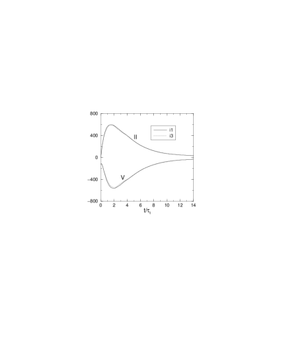
Figure 4: Important terms in equation 3 for isotropic turbulence cases.

For the shear flow simulations, term I, production due to the mean shear is also important (figure 5). However, for the value of $S_{0}^{*}$ considered for this study, this term is smaller than term II. Unlike the isotropic cases, for the shear flow cases $M_{t_{0}}$ has a strong influence on the evolution of the terms in equation 3 (figure 5a). The production terms and the dissipation term decrease their values significantly as $M_{t_{0}}$ increases. However, the decrease in the viscous dissipation term leads to an increase in the values of $\xi$. Therefore, the reduction in $\xi$ at higher $M_{t_{0}}$ is due to a decrease in the production terms, primarily due to the reduction of term II. Similarly, all terms in equation 3 decrease their values for the reacting cases as compared to the nonreacting case (figure 5b). Nevertheless, during the time when the reaction is significant, the reduction in the production terms (mainly term II) is responsible for the decrease in $\xi$.

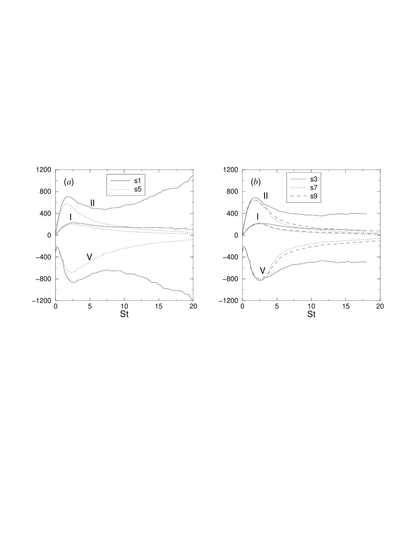
Figure 5: a) Mach number and b) heat release effect on the terms in equation 3.

The results presented suggest that the reduction in the values of $\xi$ (and hence $\epsilon_{Z}$ for the nonreacting cases) can be associated mainly to a decrease in the production due to the solenoidal strain. This term is dependent on the relative orientation between the mixture fraction gradient and the solenoidal strain rate tensor, the magnitude of the corresponding eigenvalues and the mixture fraction gradient variance. For compressible isotropic turbulence, Jaberi, Livescu & Madnia (2000) showed that the scalar gradient tends to align with the most compressive eigenvector of the strain rate tensor, similar with the behavior observed earlier in incompressible turbulence (Ashurst et al. 1987). Our results indicate that this alignment is also obtained with the solenoidal part of the strain rate tensor and it does not change significantly with increasing $M_{t_{0}}$.

However, for the shear flow simulations the PDF of the cosine of the angle between $\nabla Z^{\prime\prime}$ and the $\gamma$-eigenvector of $\underline{\underline{s^{s}}}$ peaks at a value different than 1, indicating a most probable distribution towards an angle different than zero (figure 6). $\chi_{1}$, $\chi_{2}$, and $\chi_{3}$, are angles between $\nabla Z^{\prime\prime}$ and the $\alpha$-, $\beta$-, and $\gamma$-eigenvectors, respectively. These eigenvectors correspond to the eigenvalues labeled using the usual convention $\alpha>\beta>\gamma$. For a homogeneous flow, $<\alpha>+<\beta>+<\gamma>=0$. Since $<\alpha>>0$, it has a negative contribution to the magnitude of the production term (term II in equation 3), while $<\gamma>$ has a positive contribution. For all cases considered $<\beta>>0$ and it is small compared to $<\alpha>$ and $<\gamma>$. As the initial turbulent Mach number increases, the peak of the PDF of $\cos\chi_{3}$ moves to smaller values, so the alignment worsens (figure 6a), contributing to a decrease in the production term. Furthermore, the peak of the PDF of $\cos\chi_{1}$ tends to occur at higher values as $M_{t_{0}}$ increases, so that the alignment with the most dilatational eigenvalue improves, further decreasing the production term. Moreover, all three eigenvalues of the solenoidal strain rate tensor decrease their magnitude at higher $M_{t_{0}}$ and it can be shown that this effect also contributes to the decrease in the production term.

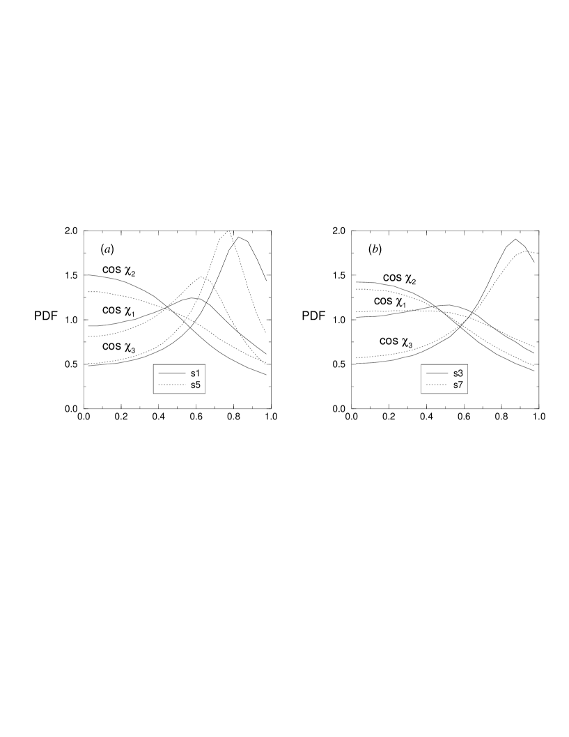
Figure 6: PDFs of the cosines of the angles between the eigenvectors of the solenoidal strain rate tensor and the mixture fraction gradient. a) Mach number effect ($St=8$) and b) heat release effect ($St=6$).

For the reacting cases, near the time when the reaction rate peaks, the alignment between $\nabla Z^{\prime\prime}$ and the $\gamma$-eigenvector improves slightly (the peak of the PDF of $\cos\chi_{3}$ moves to higher values), which has a positive contribution to the production term (figure 6b). Later, the alignment becomes close to that obtained for the nonreacting cases. However, the decrease in the magnitudes of the eigenvalues is more significant and the production term has smaller values than in the nonreacting case.

4 Conclusion

DNS of compressible homogeneous turbulent shear flow and isotropic decaying turbulence are performed under reacting (heat releasing) and nonreacting conditions to examine the role of compressibility and heat release on the scalar mixing. For the reacting cases the chemical reaction is modeled as one step, irreversible, and Arrhenius type. The statistics pertaining to the mixture fraction are extracted from the reacting scalars and compared to those obtained for a passive scalar in the nonreacting cases.

For the range of $M_{t_{0}}$ examined, it is found that the mixture fraction dissipation rate is less sensitive to the changes in $M_{t_{0}}$ in isotropic turbulence than in shear flow. For the shear flow cases $\epsilon_{Z}$ is strongly affected by compressibility and it decreases as $M_{t_{0}}$ increases. Although $\epsilon_{Z}$ increases for the reacting cases during the time when the reaction is important, this is primarily due to the increase in the viscosity. Similar with the Mach number effect, the mixture fraction gradient variance decreases for the reacting cases. The mechanical to scalar dissipation time scale ratio is also dependent on $M_{t_{0}}$ in shear flow, unlike the isotropic turbulence where the dependence was found to be weak.

The transport equation for the normalized mixture fraction gradient variance was examined and was found that the explicit dilatational terms are much smaller than the other terms in the equation. For the shear flow simulations, the mixture fraction gradient variance decreases with Mach number primarily due to a misalignment between the mixture fraction gradient and the eigenvectors of the solenoidal strain rate tensor, and also a decrease in the magnitudes of the corresponding eigenvalues. However, for the reacting cases the normalized scalar gradient variance decreases mainly due to a reduction in the eigenvalues of the solenoidal strain rate tensor.

References

- [1] Ashurst, W. T., Kerstein, A. R., Kerr, R. M & Gibson, C. H. 1987 Alignment of vorticity and scalar gradient with strain rate in simulated Navier-Stokes turbulence. Phys. Fluids 30, 2343-2353.
- [2] Blaisdell, G. A., Mansour, N. N. & Reynolds, W. C. 1994 Compressibility effects on the passive scalar flux within homogeneous turbulence. Phys. Fluids 6, 3498-3500.
- [3] Cai, X. D., O’Brien, E. E. & Ladeinde, F. 1998 Advection of mass in forced, homogeneous, compressible turbulence. Phys. Fluids 10, 2249-2259.
- [4] Jaberi, F. A., Miller, R. S., Madnia, C. K. & Givi, P. 1996 Non-Gaussian scalar statistics in homogeneous turbulence. J. Fluid Mech. 313, 241-282.
- [5] Jaberi, F. A., Livescu, D. & Madnia, C. K. 2000 Characteristics of chemically reacting compressible homogeneous turbulence. Physics of Fluids 12, 1189-1209.
- [6] Livescu, D., Jaberi, F. A. & Madnia, C. K. 2000 Passive scalar wake behind a line source in grid turbulence. J. Fluid Mech. 416, 117-149.
- [7] Livescu, D., Jaberi, F. A. & Madnia, C. K. 2001 Heat release effects on the energy exchange in reacting turbulent shear flow. To appear in J. Fluid Mech.
- [8] Overholt, M. R. & Pope, S. B 1996 Direct numerical simulation of a passive scalar with imposed mean gradient in isotropic turbulence. Phys. Fluids 8, 3128-3148.
- [9] Ristorcelli, J. R. & Blaisdell, G. A. 1997 Consistent initial conditions for the DNS of compressible turbulence. Phys. Fluids 9, 4-6.
- [10] Slessor M. D., Bond C. L. & Dimotakis P. E. 1998 Turbulent shear-layer mixing at high Reynolds numbers: effects of inflow conditions. J. Fluid Mech. 376, 115-138.
- [11] Xu, G., Antonia, R. A. & Rajagopalan, S. 2000 Scaling of mean temperature dissipation rate. Phys. Fluids 12, 3090-3093.