Dipolar Relaxation of Cold Sodium Atoms in
a Magnetic Field

Abstract

A quantum mechanical close coupling theory of spin relaxation in the stretched $F=2,M_{F}=2$, hyperfine level of sodium is presented. We calculate the dipolar relaxation rate of magnetically trapped cold sodium atoms in the magnetic field range $\rm 0<B<4\,Tesla$. The influence of shape resonances and the anisotropy of the dipolar interaction on the collision dynamics are explored. We examine the sensitivity of the calculated cross sections on the choice of asymptotic atomic state basis. We calculate and compare elastic scattering with dipolar relaxation cross sections for temperatures ranging from the ultra-cold to $\rm 2\,K$. We find that the value for the ratio of elastic to inelastic cross sections favor application of proposed buffer gas cooling and loading schemes.

I introduction

Advances in the cooling and trapping of atoms have greatly facilitated the exploration of quantum degenerate matter leg01 . The realization of Bose-Einstein condensation (BEC) and95 ; dav95 ; brad95 ; fried98 in atomic vapors validates the standard theory huang57 for non-interacting and weakly interacting systems, but experiments kett98 ; cour98 ; rob98 demonstrate that atomic interactions, though weak in an ensemble of atoms in the gas phase, lead to interesting phenomena that are not present in the ideal gas system moer95 ; kett99 ; rob00 ; don01 .

In a dilute, cold, gas, atoms interact primarily via long range dispersion and exchange forces. However, inelastic processes are driven by spin exchange dalg61 ; zyg03 and dipolar interactions ver86 . The latter process does not conserve total, atom pair, spin angular momentum and it is a primary mechanism by which atoms, having hyperfine structure, can suffer an inelastic transition. Dipolar relaxation determines the lifetime of the hydrogen atom BEC grey00 , contributes to heating and influences the operation of atomic clocks kok97 . Rates for dipolar relaxation have been measured in $\rm{}^{7}Li$ hul99 , $\rm Cs$ sod98 , $\rm{}^{85}Rb$ rob00 , $\rm H$ grey00 and $\rm Cr$ wein01 . The rates are generally small, typically having values that range $10^{-14}-10^{-16}\,cm^{3}s^{-1}$, but in the cases of $\rm Cs$ and $\rm Cr$ anomalously large values have been reported sod98 ; wein01 ; decarv03 . Calculations for dipolar relaxation rates, in the zero temperature limit, of several species have also been reported stoof88 ; ver86 ; ver91 ; ver93 ; ver96 ; mies96 ; mies00 .

New magnetic trapping and buffer gas cooling schemes doy99 ; harris03 create the opportunity to study a host of atomic and molecular species that are not amenable to laser cooling technology. In a typical loading scheme, species with large magnetic moments are trapped by external fields at relatively high temperatures, on the order of 1 K, before they are cooled into the sub-Kelvin regime. In order to model this process one needs a detailed understanding of the collision processes that can lead to trap loss and heating. To that end, we present a comprehensive quantum mechanical theory of dipolar relaxation in alkali atoms. The theory is suited for application in gases at temperatures where many partial waves in the collision wave function contribute, and is applicable at arbitrary external magnetic field intensity. We apply the theory to calculate the dipolar relaxation rate of the stretched hyperfine level in the $\rm{}^{23}Na(3s)$ atom and, in this paper, present results for temperatures that range from the ultra-cold to several Kelvin and magnetic field intensities in the range $\rm 0<B<4\,\rm Tesla$. The results of our calculation are compared to previous theoretical predictionsver91 ; ver96 . We present, the first fully quantum mechanical calculation for dipolar relaxation of sodium atoms in a magnetic field at higher temperatures where many partial waves contribute. We give a detailed description of the collision theory and explore the consequences of anisotropy on the collision dynamics. We point out the importance of shape resonances and their influence on the value of the inelastic rate. We identify a feature in the cross section that corresponds to the presence of an above threshold resonance, or a virtual state, in the $l=2$ partial wave of the scattering amplitude.

In section I we provide an introduction to the theoretical formalism that is applied in the calculations. A detailed discussion of the close coupling equations, asymptotic boundary conditions and symmetry requirements is given in sections II, and III. In section IV we present the results of our calculations, and provide a detailed analysis of these results. Unless it is otherwise stated, atomic units are used throughout the discussion.

II Channel basis

We consider two sodium atoms in their $F=2,\,M_{F}=2$ hyperfine level, the maximal stretched state. In Table I we itemize two-atom hyperfine levels with the notation $|FM_{F}f_{a}f_{b}>$, where $F$ is the total angular momentum of the two atoms, $M_{F}$ the azimuthal projection of that angular momentum, and $f_{a}$, $f_{b}$ are the total angular momenta for atoms $a$ and $b$ respectively. The states listed can mix, through dipolar and spin exchange interactions, with the maximal stretched state during a collision.

Table 1: Quantum numbers associated with the various basis representations. $M_{F}$ is the total spin angular momentum along the quantization axis and $\Delta_{F}$ is the energy defect between the $F=2$ and $F=1$ hyperfine levels in Sodium.

$M_{F}$	index	$|f_{a}m_{a}f_{b}m_{b}>$	level	Energy	$|FM_{F}f_{a}f_{b}>$	$|SM_{S}IM_{I}>$
4	1	2 2 2 2	h h	$2\Delta_{F}$	4 4 2 2	1 1 3 3
3	2	2 2 2 1	h g	$2\Delta_{F}$	4 3 2 2	1 1 3 2
3	3	2 1 2 2	h g	$2\Delta_{F}$	3 3 2 2	1 0 3 3
3	4	2 2 1 1	h a	$\Delta_{F}$	3 3 2 1	1 1 2 2
3	5	1 1 2 2	h a	$\Delta_{F}$	3 3 1 2	0 0 3 3
2	6	2 2 2 0	h f	$2\Delta_{F}$	4 2 2 2	1 1 3 1
2	7	2 0 2 2	h f	$2\Delta_{F}$	3 2 2 2	1 0 3 2
2	8	2 2 1 0	h b	$\Delta_{F}$	3 2 2 1	1 1 2 1
2	9	1 0 2 2	h b	$\Delta_{F}$	3 2 1 2	1 0 2 2
2	10	2 1 2 1	g g	$2\Delta_{F}$	2 2 2 2	1 -1 3 3
2	11	1 1 2 1	g a	$\Delta_{F}$	2 2 1 2	1 1 1 1
2	12	2 1 1 1	g a	$\Delta_{F}$	2 2 2 1	0 0 3 2
2	13	1 1 1 1	a a	$0$	2 2 1 1	0 0 2 2

Dipolar interaction selection rules(discussed in the sections below), allow a change in the azimuthal quantum number $\Delta_{M_{F}}=2,1$ and thus the states itemized in Table I must be included in the close coupling expansion. States within a given $M_{F}$ manifold can undergo spin-exchange transitions. In Table I we also list the basis $|f_{a}m_{a}f_{b}m_{b}>$ in which the individual atom azimuthal angular momenta are good quantum numbers. The basis $|SM_{S}IM_{I}>$ diagonalizes the asymptotic Hamiltonian if the hyperfine interaction can be neglected, i.e. at large magnetic field strengths. Here, $S,\,M_{S}$ are the total two-atom spin angular momentum quantum numbers, and $I,M_{I}$ the nuclear angular momentum quantum numbers. Allowed values for $\rm{}^{23}Na_{2}$ are $S=1,0$ and $I=3,2,1,0$. In the close coupling expansion involving molecular channel states we keep the notation that is appropriate for the asymptotic region to itemize the states in the expansion. For example, we define molecular channel basis $|SM_{S}IM_{I}>\equiv|^{3}\Sigma_{u}>\otimes|IM_{I}>$ for $S=1$, and $|SM_{S}IM_{I}>\equiv|^{1}\Sigma_{g}>\otimes|IM_{I}>$ for $S=0$, where $|^{3}\Sigma_{u}>,|^{1}\Sigma_{g}>$ are Born-Oppenheimer (BO) eigenstates for the ground $\rm Na_{2}$ system. The molecular channel basis merge to the correct asymptotic basis at large inter-nuclear separation. The states $|FM_{F}f_{a}f_{b}>$ are then defined by the linear combination of the BO channel states given above,

$$|FM_{F}f_{a}f_{b}>\equiv\sum|SM_{S}IM_{I}><M_{I}IM_{S}S|FM_{F}f_{a}f_{b}>$$ (1)

where the coefficients $<M_{I}IM_{S}S|FM_{F}f_{a}f_{b}>$ are standard recoupling coefficients appropriate for the asymptotic basis. In this way we insure the molecular close coupling expansion accounts for the asymptotic hyperfine interaction within each atom. In the case of a homonuclear system, the basis $|FM_{F}f_{a}f_{b}>$ is not an eigenstate of the electron inversion operator, but we can define the states $|FM_{F}(f_{a}f_{b})>\equiv{1\over\sqrt{2}}(|FM_{F}f_{a}f_{b}>\pm|FM_{F}f_{b}f_{a}>$, that are eigenstates.

In a non-zero magnetic field, the asymptotic Hamiltonian is not diagonal in the representation defined by the basis vectors introduced above. In addition to asymptotic hyperfine interactions, each atom experiences the Zeeman interaction. In that case, a linear combination of the basis states defined above must be found so that the asymptotic Hamiltonian is diagonal in the new representation. We express these states using the notation $|M_{F}\,p\,\epsilon_{i}>$, where $M_{F}$ is the total angular momentum along the direction fixed by the magnetic field, $p$ is an inversion parity quantum number, and $\epsilon_{i}$ is the asymptotic energy level eigenvalue. We discuss the construction of that basis in the sections below.

In Figs. 1a,1b we illustrate the energy spectrum of the asymptotic Hamiltonian for the $\rm Na_{2}$ system, as a function of magnetic field strength.

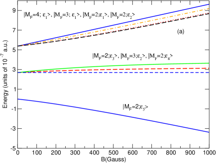
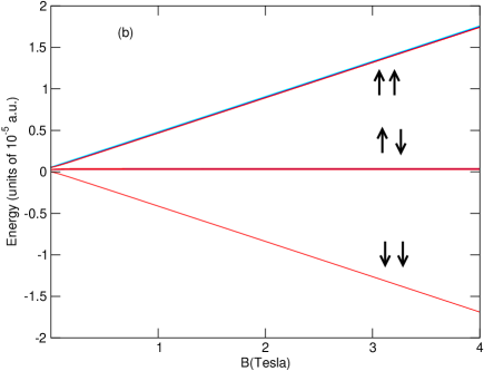
Figure 1: (a) Energy levels for a pair of sodium atoms in a magnetic field. The levels correspond to the states itemized in Table II. In the figure they are grouped in order of decreasing energy. (b) In the large $B$ field limit the arrows represent the total electronic, azimuthal, spin angular momentum of the corresponding levels shown.

III Close coupling expansion

In the Pauli approximation, the magnetic Breit interaction between the two valence electrons is given by bs57

$$\alpha^{2}\Biggl{[}-{8\pi\over 3}{\bf S}_{1}\cdot{\bf S}_{2}\,\delta^{3}({\bf r}_{12})+{1\over r_{12}^{3}}\Bigl{\{}{\bf S}_{1}\cdot{\bf S}_{2}-3{{\bf S}_{1}\cdot{\bf r}_{12}\,{\bf S}_{2}\cdot{\bf r}_{12}\over r_{12}^{2}}\Bigl{\}}\Biggr{]}$$ (2)

where $\alpha$ is the fine structure constant, ${\bf S}_{i}$ the spin of electron $i$ and ${\bf r}_{ij}$ the displacement vector for the two electrons. In order to include the magnetic interactions in the scattering equations we substitute ${\bf r}_{ij}\rightarrow{\bf R}$, where ${\bf R}$ is the inter-nuclear vector of the two atoms. This approximation is valid at large inter-nuclear separations and we replace expression (2) by the model interaction

$$H_{di-polar}\equiv{\alpha^{2}\over R^{3}}\Biggl{[}{\bf S}_{1}\cdot{\bf S}_{2}-3{({\bf S}_{1}\cdot{\bf R})({\bf S}_{2}\cdot{\bf R})\over{R^{2}}}\Biggr{]}$$ (3)

where we have ignored the Fermi-contact term. We did not include the electron spin-nuclear spin and the nuclear spin-nuclear spin interactions since they contribute to the interaction energy an amount that is at least three orders of magnitude smaller than the interaction energy obtained from Eq. (3).

Using standard Racah-algebra techniques, we re-express $H_{di-polar}$ in terms of irreducible tensor operators, thus weis78

$$H_{di-polar}=v(R)\sum_{q}(-1)^{q}{Y^{(2)}}_{q}(\theta\phi)S^{(2)}_{-q}$$ (4)

where $Y^{(2)}_{q}$ are the components of the spherical harmonic of rank 2, $S^{(2)}$ is a second rank tensor in the product space spanned by the states $|S_{1}m_{1}S_{2}m_{2}>$, and $v(R)\equiv-\sqrt{24\pi\over 5}{\alpha^{2}\over R^{3}}$ expressed in atomic units.

In the special of case of a null external magnetic field, both $|FM_{F}f_{a}f_{a}>$ and $|f_{a}m_{a}f_{b}m_{b}>$ basis vectors, itemized in Table I, diagonalize the total Hamiltonian in the asymptotic region. We use the former set to express the system wavefunction by the close coupling expansion,

$$\Psi({\bf R},{\bf r})=\sum F_{FM_{F}f_{a}f_{b}}({\bf R})|FM_{F}f_{a}f_{b}>$$ (5)

where the sum is over all quantum numbers itemized in Table I, and from which we obtain the coupled equations,

$$-{1\over 2\mu}{\nabla^{2}}F_{i}({\bf R})+\sum_{j}V^{e}_{ij}(R)F_{j}({\bf R})+\sum_{j}V^{hf}_{ij}F_{j}({\bf R})+\sum_{j}V^{m}_{ij}({\bf R})F_{j}({\bf R})=EF_{i}({\bf R}).$$ (6)

In deriving Eq.(6) we have ignored non-adiabatic effectszyg03 ; wol83 , since they are expected to provide a small correction in the sodium-sodium system. The subscript on the scattering amplitude denotes the channel quantum numbers, $i\equiv({FM_{F}f_{a}f_{b}})_{i}$, $E$ is the total energy, and $V^{e}_{ij}(R)$, $V^{hf}_{ij}(R)$, $V^{m}_{ij}({\bf R})$ are multi-channel potentials that correspond to the electrostatic, nuclear hyperfine, and di-polar magnetic interaction Hamiltonian respectively. The explicit electrostatic and hyperfine terms are

$${V_{ij}}^{e}(R)=\sum_{SI}(-1)^{f_{a}+f_{b}+f^{\prime}_{a}+f^{\prime}_{b}}\,\delta_{F,F^{\prime}}\,\delta_{M_{F},M_{F^{\prime}}}[F,S,I][f_{a},f_{a^{\prime}},f_{b},f_{b^{\prime}}]^{1/2}\times$$

$$\begin{Bmatrix}1/2&3/2&f_{a}\cr 1/2&3/2&f_{b}\cr S&I&F\end{Bmatrix}\begin{Bmatrix}1/2&3/2&f_{a^{\prime}}\cr 1/2&3/2&f_{b^{\prime}}\cr S&I&F\end{Bmatrix}\epsilon_{S}(R)$$ (7)

$${V_{ij}}^{hf}=\delta_{ij}{A_{f}\over 2}\bigl{[}f_{a}(f_{a}+1)+f_{b}(f_{b}+1)\bigr{]}$$ (8)

where $A_{F}$ is the Fermi hyperfine constant for the ground state of sodium, $\mu$ is the nuclear reduced masszyg03 ; wol83 , and $\epsilon_{S}(R)$ are the $\rm Na_{2}$ ground state Born-Oppenheimer potentials, for the triplet $S=1$, and singlet $S=0$ states respectively. In deriving Eq. (7) we used the relation

$$<IM_{I}SM_{S}|FM_{F}f_{a}f_{b}> = [F,f_{a},f_{b},S,I]^{1/2}(-1)^{F+M_{F}}\times$$

$$\begin{pmatrix}S&F&I\cr M_{S}&-M_{F}&M_{I}\end{pmatrix}\begin{Bmatrix}1/2&3/2&f_{a}\cr 1/2&3/2&f_{b}\cr S&I&F\end{Bmatrix}.$$ (9)

We now derive an expression for the di-polar interaction. Using Eq. (4) we have

$$V^{m}_{ij}({\bf R})=v(R)\sum_{q}(-1)^{q}Y^{(2)}_{q}(\theta\phi)<f_{a^{\prime}}f_{b^{\prime}}M_{F^{\prime}}F^{\prime}|S^{(2)}_{-q}|FM_{F}f_{a}f_{b}>$$ (10)

but

$$<f_{a^{\prime}}f_{b^{\prime}}M_{F^{\prime}}F^{\prime}|S^{(2)}_{-q}|FM_{F}f_{a}f_{b}>=\sum_{SM_{S}IM_{I}}\sum_{S^{\prime}M_{S^{\prime}}I^{\prime}M_{I^{\prime}}}(-1)^{F+F^{\prime}+M_{F}+M_{F^{\prime}}}\delta_{I,I^{\prime}}\delta_{M_{I},M_{I^{\prime}}}\times$$

$${[F,F^{\prime},S,S^{\prime},I,I^{\prime},f_{a},f_{a^{\prime}},f_{b},f_{b^{\prime}}]}^{1/2}<SM_{s}|S^{(2)}_{-q}|S^{\prime}M_{S^{\prime}}>\begin{Bmatrix}S&F&I\cr M_{S}&-M_{F}&M_{I}\end{Bmatrix}\times$$

$$\begin{pmatrix}S^{\prime}&F^{\prime}&I\cr M_{S^{\prime}}&-M_{F^{\prime}}&M_{I}\end{pmatrix}\begin{Bmatrix}1/2&3/2&f_{a}\cr 1/2&3/2&f_{b}\cr S&I&F\end{Bmatrix}\begin{Bmatrix}1/2&3/2&f_{a^{\prime}}\cr 1/2&3/2&f_{b^{\prime}}\cr S^{\prime}&I^{\prime}&F^{\prime}\end{Bmatrix}$$ (11)

and since

$$<SM_{s}|S^{(2)}_{-q}|S^{\prime}M_{S^{\prime}}> = (-1)^{S-M_{S}}\begin{pmatrix}S&2&S^{\prime}\cr-M_{S}&-q&M_{S^{\prime}}\end{pmatrix}<S||S^{(2)}||S^{\prime}>=$$ (12)

$$\delta_{S,S^{\prime}}\delta_{S,1}\sqrt{{15\over 12}}(-1)^{M_{S}+1}\begin{pmatrix}S&2&S\cr-M_{S}&-q&M_{S^{\prime}}\end{pmatrix}$$

we get

$$<f_{a^{\prime}}f_{b^{\prime}}M_{F^{\prime}}F^{\prime}|S^{(2)}_{-q}|FM_{F}f_{a}f_{b}> = \sum_{M_{S}M_{S^{\prime}}}\sum_{IM_{I}}(-1)^{F+F^{\prime}+M_{F}+M_{F^{\prime}}+M_{S}+1}\times$$

$${[F,F^{\prime},f_{a},f_{a^{\prime}},f_{b},f_{b^{\prime}}]}^{1/2}\sqrt{{15\over 12}} \begin{pmatrix}1&2&1\cr-M_{S}&-q&M_{S^{\prime}}\end{pmatrix}\begin{pmatrix}1&F&I\cr M_{S}&-M_{F}&M_{I}\end{pmatrix}\times$$

$$\begin{pmatrix}1&F^{\prime}&I\cr M_{S^{\prime}}&-M_{F^{\prime}}&M_{I^{\prime}}\end{pmatrix} \begin{Bmatrix}1/2&3/2&f_{a}\cr 1/2&3/2&f_{b}\cr 1&I&F\end{Bmatrix}\begin{Bmatrix}1/2&3/2&f_{a^{\prime}}\cr 1/2&3/2&f_{b^{\prime}}\cr 1&I&F^{\prime}\end{Bmatrix}.$$ (13)

Therefore,

$$V^{m}_{ij}({\bf R}) = \sum_{q}(-1)^{q}Y^{(2)}_{q}(\theta\phi)v_{ij}(q,R)$$

$$v_{ij}(q,R) \equiv v(R)\sum_{M_{S}M_{S^{\prime}}}\sum_{IM_{I}}(-1)^{F+F^{\prime}+M_{F}+M_{F^{\prime}}+M_{S}+1}{[F,F^{\prime},f_{a},f_{a^{\prime}},f_{b},f_{b^{\prime}}]}^{1/2}\times$$

$$\begin{pmatrix}1&2&1\cr-M_{S}&-q&M_{S^{\prime}}\end{pmatrix} \begin{pmatrix}1&F&I\cr M_{S}&-M_{F}&M_{I}\end{pmatrix}\begin{pmatrix}1&F^{\prime}&I\cr M_{S^{\prime}}&-M_{F^{\prime}}&M_{I}\end{pmatrix}\times$$ (14)

$$\sqrt{{45\over 4}}\begin{Bmatrix}1/2&3/2&f_{a}\cr 1/2&3/2&f_{b}\cr 1&I&F\end{Bmatrix}\begin{Bmatrix}1/2&3/2&f_{a^{\prime}}\cr 1/2&3/2&f_{b^{\prime}}\cr 1&I&F^{\prime}\end{Bmatrix}.$$

We express amplitude (5) by a partial wave expansion in spherical harmonics,

$$F_{i}({\bf R})=\sum_{lm}{F_{i}(lm,R)\over R}Y_{lm}(\theta\phi).$$ (15)

Though $V_{ij}^{e},\,V_{ij}^{hf}$ are isotropic in the nuclear orientation $V_{ij}^{m}$, according to Eq. (14), is not and the partial wave expansion does not lead to radial equations that are diagonal in the nuclear angular momentum $l$ and $m$. Inserting (15) into Eq. (6) we obtain,

$$-{1\over 2\mu}\bigl{(}{d^{2}\over dR^{2}}-{l(l+1)\over R^{2}}\bigr{)}F_{i}(lm,R)+\sum_{j}V^{e}_{ij}(R)F_{j}(lm,R)+\sum_{j}V^{hf}_{ij}F_{j}(lm,R)+$$

$$\sum_{j}\sum_{l^{\prime},m^{\prime}}u_{ij}(lm,l^{\prime}m^{\prime},R)F_{j}(l^{\prime}m^{\prime},R)=EF_{i}(lm,R)$$ (16)

where,

$$u_{ij}(lm,l^{\prime}m^{\prime},R) = ({[l,l^{\prime},2]\over 4\pi})^{1/2}\sum_{q}v_{ij}(q,R)(-1)^{q+m}\begin{pmatrix}l&2&l^{\prime}\cr-m&q&m^{\prime}\end{pmatrix}\begin{pmatrix}l&2&l^{\prime}\cr 0&0&0\end{pmatrix}$$ (17)

According to Eq. (14) $q=M_{F}-M_{F^{\prime}}\equiv\Delta M_{F}$, and from Eq. (17) $q=m-m^{\prime}\equiv\Delta m$. Therefore we obtain the selection rule $\Delta m=\Delta M_{F}$ and from the selection rules for the $3j$ symbols in Eq. (16) we require $l-l^{\prime}\equiv\Delta l=0,2$ , and $l=l^{\prime}\neq 0$.

IV Scattering formalism

It is useful to re-express the coupled radial equations in the form

$$-{1\over 2\mu}\bigl{(}{d^{2}\over dR^{2}}-{{\underline{l}}({\underline{l}}+1)\over R^{2}}\bigr{)}{\underline{F}}(R)+{\underline{V}}^{e}(R){\underline{F}}(R)+{\underline{V}}^{hf}{\underline{F}}(R)+{\underline{V}}^{m}(R){\underline{F}}(R) =$$

$$E{\underline{F}}(R).$$ (18)

In the notation introduced above ${\underline{F}}(R)$ is a square matrix whose columns contain the independent solution vectors to the coupled equations (16). The row and column indices for matrix ${\underline{F}}(R)$ itemize both the internal and orbital angular momentum quantum numbers. A given value of index $i$, identifies the set $i\equiv\{(FM_{F}f_{a}f_{b})_{i}l_{i}m_{i}\}$ where $l_{i}$, $m_{i}$ are the total and azimuthal quantum numbers for channel $i$. At a given collision energy, we are allowed to truncate the partial wave expansion (15) at some maximum value $l_{max}$ and matrix ${\underline{F}}(R)$ is a finite $n$-dimensional square matrix where $n=n_{i}\prod_{l=0}^{l_{max}}(2l+1)$, and $n_{i}$ is the dimension of the internal Hilbert space.

Matrices ${\underline{V}}^{e}(R)$, ${\underline{V}}^{hf}$, correspond to the electrostatic and hyperfine Hamiltonian respectively, and they are diagonal with respect to the angular momentum quantum numbers. The matrix ${\underline{l}}$ is diagonal and contains the channel angular momenta along the diagonal. However, ${\underline{V}}^{m}(R)$, whose components are ${\underline{V}}^{m}_{ij}(R)=u_{ij}(l_{i}m_{i};l_{j}m_{j};R)$, is not diagonal.

In the limit $R\rightarrow\infty$ we require that

$${\underline{F}}_{ij}(R)\rightarrow{1\over\sqrt{k_{i}}}\Biggl{\{}\delta_{ij}sin(k_{i}R-l_{i}{\pi\over 2})+{\underline{K}}_{ij}cos(k_{i}R-l_{i}{\pi\over 2})\Biggr{\}}$$ (19)

where ${\underline{K}}_{ij}$ are the elements of the $K$ matrix.

We introduce the amplitude ${\underline{G}}(R)\equiv{\underline{F}}(R)\,{\underline{C}}$ where ${\underline{C}}$ is a constant matrix chosen so that in the limit $R\rightarrow\infty$

$${\underline{G}}_{ij}(R)={1\over k_{i}^{1/2}}\Biggl{\{}\delta_{ij}\exp(-i(k_{i}R-l_{i}{\pi\over 2}))-{\underline{S}}_{ij}\exp(i(k_{i}R-l_{i}{\pi\over 2}))\Biggr{\}}$$ (20)

where the radial S-matrix ${\underline{S}}$ is,

$${\underline{S}}=({\underline{I}}-i{\underline{K}})({\underline{I}}+i{\underline{K}})^{-1}$$ (21)

We construct a reduced multichannel amplitude, ${\underline{G}}_{[ij]}({\bf R})$, where the notation $[ij]$ implies that the indices denote the quantum numbers of the internal states only. We define

$${\underline{G}}_{[ij]}({\bf R})=\sum_{l_{i}m_{i}}\sum_{l_{j}m_{j}}Y_{l_{i}m_{i}}(\theta\phi)Y^{*}_{l_{j}m_{j}}(\theta_{i}\phi_{i}){2\pi i^{l_{j}+1}\over k_{j}^{1/2}}{{\underline{G}}_{ij}(R)\over R}$$ (22)

and find that in the asymptotic limit $R\rightarrow\infty$

$${\underline{G}}_{[ij]}({\bf R})\rightarrow\delta_{[ij]}\exp(i{\bf K}_{i}\cdot{\bf R})+f_{[ij]}(\theta\phi;\theta_{i}\phi_{i}){\exp(ik_{i}R)\over R}$$ (23)

where we have used Eq. (20), and $f_{[ij]}(\theta\phi;\theta_{i}\phi_{i})$ is the scattering amplitude for the system to undergo a transition from an initial internal state $j$ into an internal state $i$ and into solid angle $d\theta(sin\theta)d\phi$ following an initial approach along the incident wave vector ${\bf K}_{i}$ with polar angles $\theta_{i}\phi_{i}$. Comparing expression (22) and (23) we find that

$$f_{[ij]}(\theta\phi;\theta_{i}\phi_{i})\equiv\sum_{l_{i}m_{i}}\sum_{l_{j}m_{j}}Y_{l_{i}m_{i}}(\theta\phi)Y^{*}_{l_{j}m_{j}}(\theta_{i}\phi_{i}){2\pi i^{l_{j}+1}\over k_{i}^{1/2}k_{j}^{1/2}}(\delta_{ij}-{\underline{S}}_{ij}).$$ (24)

Though ${\underline{G}}_{[ij]}({\bf R})$ has the desired asymptotic behavior for scattering solutions it does not posses the symmetry required by the Pauli principle. Because the sodium nuclei are identical fermions, the total wavefunction must be odd under their interchange. Let $P^{N}_{12}$ be the nuclear permutation operator, thenzyg94

$$P^{N}_{12}|FMf_{a}f_{b}>=(-1)^{F+f_{a}+f_{b}+1}|FMf_{b}f_{a}>.$$ (25)

We introduce a shorthand notation for the channel indices that label the matrix ${\underline{G}}({\bf R})$; if $i={FMf_{a}f_{b}}$ then ${\tilde{i}}\equiv{FMf_{b}f_{a}}$. In this notation the above relation is written $P^{N}_{12}|i>=(-1)^{F+f_{a}+f_{b}+1}|{\tilde{i}}>$. If the system is initially prepared in state $j$, and is given by $|\Psi>=\sum_{i}G_{[ij]}({\bf R})|i>$ , then we require that $G_{[ij]}(-{\bf R})=(-1)^{F+f_{a}+f_{b}}G_{[{\tilde{i}}j]}({\bf R})$.

Using this notation we replace (22) with,

$$G_{[ij]}({\bf R})\equiv\sum_{l_{i}m_{i}}\sum_{l_{j}m_{j}}Y_{l_{i}m_{i}}(\theta\phi)Y^{*}_{l_{j}m_{j}}(\theta_{i}\phi_{i}){2\pi i^{l_{i}+1}\over k_{j}^{1/2}}\times$$

$$\Biggl{\{}{G_{ij}(R)\over R}+(-1)^{F+l_{i}+f_{a}+f_{b}}{G_{{\tilde{i}}j}(R)\over R}\Biggr{\}}$$ (26)

which has the desired symmetry.

In the asymptotic limit we get,

$$G_{[ij]}({\bf R}) \rightarrow \delta_{[ij]}\exp(i{\bf K}_{i}\cdot{\bf R})+(-1)^{F+f_{a}+f_{b}}\delta_{[{\tilde{i}}j]}\exp(-i{\bf K}_{i}\cdot{\bf R})+$$

$$\Bigl{[}f_{[ij]}(\theta\phi;\theta_{i}\phi_{i}) + (-1)^{F+f_{a}+f_{b}}f_{[{\tilde{i}}j]}(-\theta+\pi\,\phi+\pi;\theta_{i}\phi_{i})\Bigr{]}{\exp(ik_{i}R)\over R}$$ (27)

where we have used $k_{i}=k_{{\tilde{i}}}$. The cross section for a system in an internal state $|j>=|F^{\prime}M^{\prime}f_{a^{\prime}}f_{b^{\prime}}>$ to undergo a transition into state $|i>=|FMf_{a}f_{b}>$ is

$$\sigma(j\rightarrow i) = {v_{i}\over v_{j}}{1\over 2}\,{1\over 4\pi}\times$$ (28)

$$\int d{\hat{\bf\Omega}}\int d{\hat{\bf\Omega_{i}}}|f_{[ij]}(\theta\phi;\theta_{i}\phi_{i})+(-1)^{F+f_{a}+f_{b}}f_{{[\tilde{i}}j]}(-\theta+\pi\,\phi+\pi;\theta_{i}\phi_{i})|^{2}$$

where we integrate over all scattering angles and average over all directions of the incident wave. $v_{j}$ is the velocity in the incoming channel and $v_{i}$ the final channel velocity. We have included a factor of ${1\over 2}$ in order to insure that the incoming flux is normalized to unity. Using expression (26) we can re-write Eq. (27),

$$\sigma(j\rightarrow i) = {\pi\over 2k^{2}_{j}}\sum_{l_{i}m_{i}}\sum_{l_{j}m_{j}}|T_{[ij]}(l_{i}m_{i};l_{j}m_{j})+(-1)^{F+f_{a}+f_{b}+l_{i}}T_{[{\tilde{i}}j]}(l_{i}m_{i};l_{j}m_{j})|^{2}$$

$$T_{[ij]}(l_{i}m_{i};l_{j}m_{j}) \equiv \delta_{[ij]}-S_{[ij]}$$ (29)

We use Eq. (29) to calculate the total inelastic transition cross section in the case for zero, or small, magnetic field intensities. The initial state corresponds to the maximal extended state $|F=4\,M=4\,f_{a}=2\,f_{b}=2>$ and at low energies only incident s-waves contribute. According to the dipolar selection rules the exit channels are d-waves, and we obtain a simple expression for the total inelastic cross section

$$\sigma_{T}=\sum_{FM_{F}f_{a}f_{b}}\,\sum_{m_{i}=-2}^{m_{i}=2}{2\pi\over k^{2}}\,|{\tilde{T}}_{FM_{F}f_{a}f_{b}}(m_{i})|^{2}$$ (30)

where, ${{\tilde{T}}}_{FM_{F}f_{a}f_{b}}(m_{i})\equiv T_{[ij]}(l_{i}=2,m_{i};l_{j}=0,m_{j}=0)$ for $i={FM_{F}f_{a}f_{b}}$ and $j={F=4\,M_{F}=4,f_{a}=2\,f_{b}=2}$, and $k=k_{j}$. In deriving Eq. (30) we used the fact $T_{[{\tilde{i}}j]}=(-1)^{F+f_{a}+f_{b}}T_{[ij]}$.

For a large magnetic field, such that the Zeeman splitting is much greater than the hyperfine interaction, we construct close coupling equations by using the basis vectors $|SM_{S}IM_{I}>$ in expansion Eq. (5). We obtain an equation analogous to Eq. (18) except that ${\underline{V}}^{hf}$ is replaced by an expression that describes the Zeeman interaction with the external field. In addition, the electrostatic and dipolar interaction matrices are replaced by ${\underline{\tilde{V}}}^{e}(R)$ and ${\underline{\tilde{V}}}^{m}(R)$ respectively. They are related by the unitary transformation ${\underline{\tilde{V}}}^{e}(R)={\underline{U}}{\underline{V}}^{e}(R){\underline{U}}^{-1}$, ${\underline{\tilde{V}}}^{m}(R)={\underline{U}}{\underline{V}}^{m}(R){\underline{U}}^{-1}$, where $U_{ij}=<FM_{F}f_{a}f_{b}l_{j}m_{j}|l_{i}m_{i}SM_{S}IM_{I}>$.

Because the states $|SM_{S}IM_{I}>$ are eigenstates of the nuclear interchange operator $P_{12}^{N}$, i.e.

$$P_{12}^{N}|SM_{S}IM_{I}>=(-1)^{S+I+1}|SM_{S}IM_{I}>$$ (31)

we obtain

$$\sigma(j\rightarrow i) = {\pi\over 2k^{2}_{j}}\sum_{l_{i}m_{i}}\sum_{l_{j}m_{j}}|T_{[ij]}(l_{i}m_{i};l_{j}m_{j})(1+(-1)^{I+S+l_{i}})|^{2}$$ (32)

where the channel indices now itemize the states in Table 1 under the $|SM_{S}IM_{I}>$ representation.

If the magnetic interaction energy is of the same order as the hyperfine energy, neither the $|FM_{F}f_{a}f_{b}>$ nor the $|SM_{S}IM_{I}>$ representations constitute a valid asymptotic basis since off-diagonal elements persist at large inter-nuclear separations. Instead, we choose a linear combination of these states that diagonalize the asymptotic Hamiltonian,

$$H^{hf}+H^{Z}$$

$$H^{Z}=2{\mu_{B}}{\bf B}\cdot{\bf S}$$ (33)

where $H^{hf}$ is the hyperfine interaction, ${\bf B}$ is the external magnetic field whose orientation defines our lab quantization axis, ${\bf S}$ is the total electronic spin for the atom-atom system and $\mu_{B}$ is the Bohr magneton. We ignored the magnetic-nuclear term since it provides a considerable smaller contribution to the total magnetic interaction energy than that given by Eq. (33). The diagonalization procedure can be carried out numerically, and in Table II we itemize those states which contribute to dipolar loss from the incident, extended state, channel. Good quantum numbers for these states include the total azimuthal quantum number $M_{F}$, the nuclear interchange parity, and the energy eigenvalues $e_{i}$ itemized in Table II. The extended state is odd under nuclear interchange i.e., $P^{N}_{12}|M_{F}=4;\,p=1\,e_{1}>=(-1)^{p}\,|M_{F}=4;\,p=1\,e_{1}>$ where we have used the notation described in Table II.

Table 2: Quantum numbers associated with the states $|M_{F}\,p\,\epsilon_{i}>$ that diagonalize the asymptotic Hamiltonian, Eq. (32). We itemize only those states whose parity, under nuclear interchange, is odd. The parameter $\zeta\equiv{4\mu_{B}B\over\Delta F}$ where $B$ is the magnetic field strength and $\Delta_{F}$ the energy defect between the $F=2$ and $F=1$ hyperfine levels of Sodium. The last column itemizes the $B\rightarrow 0$ limit of the states expressed in the $|FM_{F}(f_{a}f_{b})>$ representation.

$\epsilon$	$M_{F}$	Energy	$|M_{F}\,p\,\epsilon>$
$\epsilon_{1}$	4	2 $\Delta_{F}(1+{\zeta\over 4})$	$|4422>$
$\epsilon_{1}$	3	${\Delta_{F}\over 4}(6+\zeta+\sqrt{4+2\zeta+\zeta^{2}})$	$|4322>$
$\epsilon_{2}$	3	${\Delta_{F}\over 4}(6+\zeta-\sqrt{4+2\zeta+\zeta^{2}})$	$|33(12)>$
$\epsilon_{1}$	2	${\Delta_{F}\over 2}(2+\sqrt{4+2\zeta+\zeta^{2}})$	${2\over\sqrt{7}}|4222>-\sqrt{3\over 7}|2222>$
$\epsilon_{2}$	2	${\Delta_{F}\over 4}(6+\zeta+\sqrt{4+\zeta^{2}})$	$-\sqrt{3\over 7}|4222>-{2\over\sqrt{7}}|2222>$
$\epsilon_{3}$	2	${\Delta_{F}\over 4}(6+\zeta-\sqrt{4+\zeta^{2}})$	${1\over\sqrt{3}}|32(12)>-\sqrt{2\over 3}|22(12)>$
$\epsilon_{4}$	2	$\Delta_{F}$	$-\sqrt{2\over 3}|32(12)>-{1\over\sqrt{3}}|22(12)>$
$\epsilon_{5}$	2	${\Delta_{F}\over 2}(2-\sqrt{4+2\zeta+\zeta^{2}})$	$|2211>$

Only states of odd parity are allowed as exit channels and these states are listed in Table II. Invoking the procedure discussed above, we obtain for the total dipolar loss cross section

$$\sigma_{T}=\sum_{j}\,\sum_{m_{i}=-2}^{m_{i}=2}{2\pi\over k^{2}}\,|{\tilde{T}}_{j}(m_{i})|^{2}$$ (34)

where the sum over index $j$ denotes the channels itemized in Table II.

The rate coefficient for dipolar relaxation is given by the expression

$$k_{T}=\sqrt{{8kT\over\pi\mu}}({1\over kT})^{2}\int_{0}^{\infty}dE\,E\,\sigma_{T}(E)\exp(-{E\over kT})$$ (35)

where $\mu$ is the reduced mass of the $\rm{}^{23}Na_{2}$ system and $\sigma_{T}(E)$ the total inelastic cross section expressed as a function of collision energy.

V Results and discussion

In Fig. 2 we plot the total rate coefficient(solid line), in the $T\rightarrow 0$ limit, as a function of magnetic field strength. In Fig. 2 we notice that the total relaxation rate is nearly constant for field strengths up to about 100 Gauss(G). In the range $\rm{100\,G<B<400\,G}$ the rates exhibit significant structure. For larger values of $\rm B$ the total rate diminishes in a monotonic manner. In figure 2 we also plot, shown by the dashed line, results obtained using the approximation where the hyperfine states $|FM_{F}f_{a}f_{b}>$ define the asymptotic basis states and the asymptotic off-diagonal terms, due to magnetic interactions, are neglected. For small $\rm B$ the approximation gives excellent agreement, for the total dipolar loss rate, with the results obtained using the appropriate $|M_{F}\,p\,\epsilon>$ basis. However, for ${\rm B>60\,G}$ this approximation considerably overestimates the total rate.

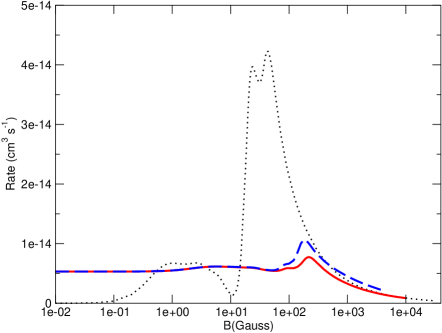
Figure 2: Total dipolar relaxation rate (heavy solid line) as a function of external magnetic field strength. The dashed lines corresponds to the approximation where the hyperfine basis $|FM_{F}f_{a}f_{b}>$ is used for the asymptotic channel states. The dotted line corresponds to the case where the $|SM_{S}IM_{I}>$ basis is used and the hyperfine interaction is ignored.

The dotted line in the figure presents the results of the calculation when we used the $|SM_{S}IM_{I}>$ representation to define the asymptotic channel basis, and where we ignored the hyperfine Hamiltonian. For small B this approximation is poor because it neglects the dominant hyperfine interaction. In the ${\rm B\rightarrow 0}$ limit, rates obtained in this approximation vanish due to the nature of the anisotropic dipolar interaction. According to the selection rules discussed in the previous sections, a pair of atoms approaching as an s-wave must exit as a d-wave, and therefore, the exit channel must be exothermic with respect to the entrance channel for the collision to proceed in the zero temperature limit. At $\rm B\rightarrow 0$ a finite energy defect is generated by the hyperfine interaction and, if hyperfine effects are ignored, the dipolar rate vanishes in the $\rm T\rightarrow 0$, limit. This effect is clearly evident in Fig. 2. As $\rm B\rightarrow\infty$ the neglect of the hyperfine interaction is justified and, in that case, we expect that the rate obtained using the $|SM_{S}IM_{I}>$ basis to be a good approximation. In Fig. 2 we note that for ${\rm B>1\,T}$ the dotted line merges with the solid line and illustrates the validity of that approximation at large field strengths.

To understand the nature of the observed structures in the total rates we neglect the fine structure and study the collision dynamics in the $|SM_{S}IM_{I}>$ basis and show the results in Fig. 3. In that figure, the dashed line denotes the partial rate into the state where both atoms flip their total electronic spin, whereas the solid line corresponds to the case where only one atom flips its spin. We first consider the kinematics of the latter case.

In the $|SM_{S}IM_{I}>$ basis the Zeeman energy splitting between the $|S=1;M_{S}=1;I=3;M_{I}>$ and the $|S=1;M_{S}=0;I=3;M_{I}>$ exit channel is given by

$$\Delta E=|2\mu_{B}{\rm B}|+{k^{2}\over 2\mu}$$ (36)

where $k$ is the wavenumber that corresponds to the kinetic energy of the system in the entrance channel and $\rm B$ is the absolute value of the magnetic field that is parallel to the laboratory z-axis. In the $k\rightarrow 0$ limit the exit channel is a d-wave and, using the potential for the ${}^{3}\Sigma_{u}$ state of $\rm{}^{23}Na_{2}$ system tabulated by Samuelis et al. sam00 , we find that the $l=2$ centrifugal barrier has a height $\Delta E(l=2)=1.6585\times 10^{-8}\,a.u.$ We equate the Zeeman splitting with the barrier height and find that the critical magnetic field strength required so enough kinetic energy is available in the exit channel to overcome the barrier has the value $\rm B_{c}=39.0\,\rm G$.

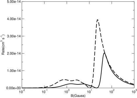
Figure 3: Resonance/threshold structures observed in the dipolar loss rates that were calculated ignoring hyperfine effects and in the $|SM_{S}IM_{I}>$ basis. The dashed line corresponds to dipolar loss involving total electronic spin flips for a single atom, whereas the solid line corresponds to spin flips involving both atoms.

According to Fig. 3, at this field strength the relaxation rate is rapidly increasing, as $\rm B$ increases, but it is in a region to the left of its maximum which occurs at $\rm B_{max}=46.0\,\rm G$. Therefore, the pronounced structure seen in this rate cannot be solely attributed to a threshold effect. Indeed we found a resonance in the $l=2$ partial wave that is due to the existence of a virtual state at $E_{v}=1.85\times 10^{-8}\,a.u.$ Using Eq. (36) to convert $E_{v}$ into a field strength, we find $\rm B^{*}=43.5\,\rm G$, a value that is about midway between $\rm B_{c}$ and $\rm B_{max}$. For transitions into the state $|S=1;M_{S}=-1;I=3;M_{I}>$, whose rate coefficient is shown by the dashed line in Fig 4, B we evaluate $\rm B^{*}={E_{v}/4\mu_{B}}$ and get $\rm B^{*}=21.8\,\rm G$. This value is close to $\rm B_{max}=23.0\,\rm G$ seen in the figure. These observations strongly suggest that the structure, evident in the in Fig. 3, is a consequence of shape resonance phenomena zyg02 ; laue02 . This conclusion is strengthened by studies, discussed below, of this collision process at higher temperatures.

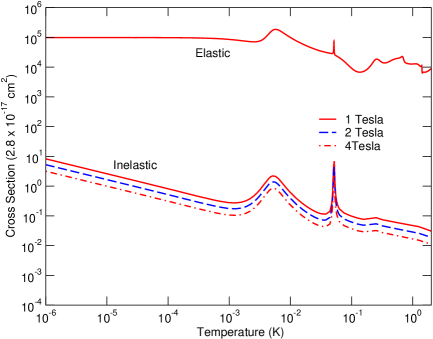
Figure 4: Elastic and inelastic cross sections in collisions of ${\rm Na}(F=2\,M_{F}=2)+{\rm Na}(F=2\,M_{F}=2).$ The collision energy is expressed in units of Kelvin.

Our rate in the $\rm B\rightarrow 0$ limit is in harmony with that that reported in a previous study ver96 , but several times larger from that predicted in an earlier study ver91 . In Refs.ver96 ; ver91 the authors used the $|f_{a}m_{a}f_{b}m_{b}>$ basis to calculate the rates for $B\neq 0$. We have shown here, that this approximation overestimates the relaxation rates for $\rm B>60\,G$. The largest uncertainty is probably associated with the choice for molecular potentials of the ground $\rm{}^{23}Na$ system. We adopted the most recent, and accurate, potentials tabulated by Samuelis et al. sam00 .

In Fig. 5 we present the results of our calculation for both the elastic and inelastic, dipolar relaxation, cross sections in collisions of spin polarized sodium atoms. The collision energies considered range from ultra-cold to 2 Kelvin. At higher temperatures many partial waves contribute and the multi-channel, close coupling theory described in the previous sections is applied. We display results obtained for magnetic fields that range between 1 and 4 Tesla. In the previous paragraphs we justified the neglect of the hyperfine interaction, in the calculations for field strengths $B>1T$. The results shown in Fig. 5 are based on this approximation, but because of the anisotropy in the dipolar interaction, this calculation still involves a large number of channels since coupled partial wave angular momenta up to $J\approx 20$ are required for convergence at temperatures $T>1K$. We find that the elastic cross sections dominate and are largely insensitive to the value of the applied field. In the range of applied fields considered and in the $\mu K$ collision energy region, the dipolar cross sections are about $10^{-3}$ smaller than the elastic cross sections. The ratio decreases at higher collision energies and at cryogenic temperatures the ratio of elastic to inelastic cross sections $\approx 10^{-6}$. At higher temperatures we find that the dipolar relaxation cross sections decrease as the applied field is increased. In Fig. 5, we note that the elastic cross sections tend to a constant value as the gas temperature approaches the $\mu\,\rm K$ range whereas the relaxation cross sections increase, in conformity with the Wigner threshold laws. Both the elastic and inelastic cross sections display resonance features discussed in the previous paragraphs. Because of the favorable ratio of elastic to inelastic cross sections, spin polarized sodium is, potentially, a good candidate for buffer gas loading and evaporative cooling.

References

• (1) Anthony J. Leggett, Rev. Mod. Phys. 73, 307 (2001).
• (2) M. H. Anderson, J. R. Ensher, M. R. Matthews, C. E. Wieman and E. A. Cornell, Science 269, 198 (1995).
• (3) K. B. Davis, M. -O. Mewes, M. R. Andrews, N. J. van Druten, D. S. Durfee, D. M. Kurn, and W. Ketterle, Phys. Rev. Lett. 75, 3969 (1995).
• (4) C. C. Bradeley, C. A. Sacket, J. J. Tollett, and R. G. Hulet, Phys. Rev. Lett. 75, 9 (1995).
• (5) D. G. Fried, T. C. Kilian, L. Willmann, D. Landhuis, S. C. Moss, D. Kleppner, and T. J. Greytak, Phys. Rev. Lett. 81, 3811 (1998).
• (6) K. Huang Statistical Mechanics, 2nd edition (Wiley, New York, 1987).
• (7) S. Inouye, M. R. Andrews, J. Stenger, H.-J. Miesner, D. M. Stamper-Kurn and W. Ketterle Nature 392, 151 (1998).
• (8) Ph. Courteille, R. S. Freeland, D. J. Heinzen, F. A. van Abeelen and B. J. Verhaar, Phy. Rev. Lett. 81, 69 (1998).
• (9) J. L. Roberts, N. R. Claussen, James P. Burke, Jr., Chris H. Greene, E. A. Cornell, and C. E. Wieman, Phys. Rev. Lett. 81, 5109 (1998).
• (10) A. J. Moerdijk, B. J. Verhaar, and A. Axelsson, Phys. Rev. A. 51, 4852 (1995).
• (11) J. Stenger, S. Inouye, M. R. Andrews, H. J. Miesner, D. M. Stemper-Kurn, and W. Ketterle, Phys. Rev. Lett. 82, 2422 (1989).
• (12) J. L. Roberts, N. R. Claussen, S. L. Cornish, and C. E. Wieman, Phys. Rev. Lett. 82 2422 (1999).
• (13) Elizabeth A. Donley, Neil R. Claussen, Simon L. Cornish, Jacob L. Roberts, Eric A. Cornell and C. E. Wieman, cond-mat/0105019 v3 1 Jun 2001.
• (14) A. Dalgarno, Proc. Roy. Soc. A, 262 132, (1961).
• (15) B. Zygelman, A. Dalgarno, M. J. Jamieson, P. C. Stancil, Phys. Rev. A 67, 042175 (2003).
• (16) L. Wolniewicz, J. Chem. Phys. 78, 6173 (1983).
• (17) Ad Lagendijk, Isaac F. Silvera, Boudewijn J. Verhaar Phys. Rev. B 33, 626 (1986).
• (18) B. Zygelman, A. Dalgarno, R. D. Sharma, Phys. Rev. A 49, 2587 (1994). In order to prove Eq. (25), we use a procedure similar to that described in the cited paper for the fine structure internal states.
• (19) T. J. Greytak, D. Kleppner, D. G. Fried, T. C. Killian, L. Willmann, D. Landhuis, S. C. Moss, Physica B 280, 20 (2000).
• (20) S. J. J. M. F. Kokkelmans and B. J. Verhaar, Phys. Rev. A 56, 4038 (1997).
• (21) J. M. Gerton, C. A. Sackett, B. J. Frew, and R. G. Hulet, Phys. Rev. A 59, 1514 (1999).
• (22) J. Soding, D. Guery-Odelin, P. Desbiolles, G. Ferrari, and J. Dalibard, PRL 80, 1869 (1998).
• (23) J. Weinstein et al. Phys. Rev. A 65, 021604 (2002).
• (24) Robert deCarvalho, Cindy I. Hancox, and John M. Doyle, J. Opt. Soc. Am. B 20, (2003).
• (25) J. G. E. Harris, R. A. Michniak, S. V. Nguyen, W. Ketterle, and J. M. Doyle, submitted Phys. Rev. Lett. 2003.
• (26) H. T. C. Stoof, J. M. V. Koelman, and B. J. Verhaar, Phys. Rev. B 38, 4688 (1988).
• (27) Mies et al., Res. Natl. Inst. Stand. Technol. 101, 521 (1996).
• (28) F. H. Mies and Raoult, Phys. Rev. A 62, 012708 (2000).
• (29) E. Tiesinga, S. J. M. Kuppens, B. J. Verhaar, and H. T. C. Stoof, Phys. Rev. A 43, 5188 (1991).
• (30) E. Tiesinga, B. J. Verhaar, and H. T. C. Stoof, Phys. Rev. A 47, 4114 (1993).
• (31) A. J. Moerdijk and B. J. Verhaar, Phys. Rev. A 53 R19 (1996).
• (32) R. deCarvalho, J. M. Doyle, B. Friedrich, T. Gillet, J. Kin, D. Patterson, and J. D. Weinstein, Eur. Phys. J. D 7, 289 (1999).
• (33) Bethe H. A. and Salpeter, E. E. (1957) Quantum Mechanics of the One-and Two-Electron Atoms,(Academic Press, New York 1957).
• (34) Mitchel Weisbluth, Atoms and Molecules, pg. 170, (Academic Press New York, 1978)
• (35) C. Samuelis, E. Tiesinga, T. Laue, M. Elbs, H. Knockel and E. Tiemann, Phys. Rev. A 63, 012710-1 (2000).
• (36) After the submission of this manuscript to this journal, it has come to our attention that there is spectroscopic evidence for an $l=2$ shape resonance in the ${}^{3}\Sigma_{u}$ state of sodium; T. Laue, E. Tiesinga, C. Samuelis, H. Knockel, and E. Tiemann, Phys. Rev. A 65, 023412 (2002).
• (37) B. Zygelman and A. Dalgarno, J. Phys. B. At. Mol. Opt. Phys. 35, L441 (2002).