Solving the boundary value problem for finite Kirchhoff rods

Abstract

The Kirchhoff model describes the statics and dynamics of thin rods within the approximations of the linear elasticity theory. In this paper we develop a method, based on a shooting technique, to find equilibrium configurations of finite rods subjected to boundary conditions and given load parameters. The method consists in making a series of small changes on a trial solution satisfying the Kirchhoff equations but not necessarily the boundary conditions. By linearizing the differential equations around the trial solution we are able to push its end point to the desired position, step by step. The method is also useful to obtain configurations of rods with fixed end points but different mechanical parameters, such as tension, components of the moment or inhomogeneities.

I Introduction

The study of conformations of slender elastic rods is of substantial utility in several applications, ranging from the fields of structural mechanics and engineering to biochemistry and biology. Examples are the study of coiling and loop formation of sub-oceanic cables coyne ; zajac ; sun ; vaz , filamentary structures of biomolecules zimm ; yang ; shi ; tamar ; golds and bacterial fibers golds2 ; klapper , the phenomenon of helix hand reversal in climbing plants goriely and the shape and dynamics of cracking whips alain3 .

The Kirchhoff model kirchhoff provides a powerful approach to study the statics and dynamics of elastic thin rods tamar ; olson . In this model the rod is described by a set of nine partial differential equations (the Kirchhoff equations) in the time and arclength of the rod. They contain the forces and torques plus a triad of vectors describing the deformations of the rod. These equations are the result of Newton’s second law for the linear and angular momentum applied to the thin rod plus a linear constitutive relationship between moments and strains. The Kirchhoff model holds true in the approximation of small curvatures of the rod, as compared to the radius of the local cross section dill . An interesting characteristic of this model, known as Kirchhoff kinetic analogy, is that the equations governing the static problem are formally equivalent to the Euler equations describing the motion of spinning tops in a gravity field. The Kirchhoff equations for equilibrium configurations can, therefore, be written in hamiltonian form.

The Kirchhoff equations have been solved for a number of simple situations. Shi and Hearstshi first obtained analytical solutions of the equilibrium equations and, recently, Nizzete and Goriely nizzete completed the study by making a classification of all kinds of equilibrium solutions. Goriely and Tabor tabor1 ; tabor2 developed a method to study the dynamical stability of these solutions and Fonseca and de Aguiar fonseca applied this method to study the near equilibrium dynamics of non-homogeneous closed rods in viscous media. Recently, Tobias et al. tobias developed the necessary and sufficient criteria for elastic stability of equilibrium configurations of closed rods.

In many cases of interest, including biological molecules, the filaments are subject to boundary conditions. Examples are the problem of multiprotein structures, such as histones and gyrase, about which long pieces of DNA wrap tobias2 , and multiprotein structures, such as the lac repressor complex mahade . Despite the many achievements described above, the study of the boundary value problem (BVP) associated with Kirchhoff filaments is still a big challenge. While the integration of differential equations from initial conditions is a relatively simple numerical task, the difficulties of finding solutions for given boundary conditions are well known in classical mechanics, electromagnetism and quantum mechanics. Typical examples are classical trajectories connecting two given space points in the time $t$, electric potentials that vanish at given surfaces and eigenvalues of the Laplace operator defined inside a finite domain (quantum billiards).

Because of the analogy with spinning tops, the case of trajectories of Hamiltonian systems is of particular interest here. The monodromy method, developed by Baranger and Davis baranger , was designed specifically to find periodic solutions of Hamiltonian systems with $N$ degrees of freedom. Xavier and de Aguiar xavier extended the method to find non-periodic trajectories with any given combination of $2N$ position and momenta at initial and/or final times.

A widely used method to solve BVPs is the so called shooting method keller ; Ha . For a single second-order differential equation, the method consists in finding the proper ’velocity’ at the initial point so as to reach the desired ’target’ at the end point, similar to the shooting of a projectile. Examples of applications of this method to the Kirchhoff equations are the search for homoclinic orbits in reversible systems spence , heteroclinic orbits resembling tendril pervesions tyler and the study of localized buckling modes of thin elastic filaments champ1 ; champ2 .

In the case of open rods some specific BVPs were solved recently. Károlyi and Domokos domokos , using symbolic dynamics, found global invariants for BVPs of elastic linkages, as natural discretization of continuous elastic beams, an old problem solved by Euler(see reference domokos ). Gottlieb and Perkins perkins investigated spatially complex forms in a BVP governing the equilibrium of slender cables subjected to thrust, torsion and gravity. Also, the criteria of Tobias et al. tobias was applied to linear segments subjected to strong anchoring end conditions, where not only the end points but also the tangent vector at the end points are held fixed. The dependence of DNA tertiary structure on end conditions was studied in tobias2 , where explicit expressions for equilibrium configurations were obtained for a specific case with symmetric end conditions.

Our aim in this paper is to develop a method to find equilibrium solutions of finite rods subjected to boundary conditions at their end points and with given load parameters. We emphasize that this is different from the approach in champ1 ; champ2 , where the authors use shooting methods to calculate localized buckling modes. These modes are treated as homoclinic solutions of the Kirchhoff equations, corresponding to infinite rods that become asymptotically straight in the infinite. Our objective is to find equilibrium solutions for finite rods subjected to boundary conditions at both ends.

Our method is an adaptation of the monodromy matrix method for non-periodic trajectories xavier to the hamiltonian formulation of the static Kirchhoff equations. We work with the Kirchhoff equations directly in Euler angles, instead of using the Cartesian position and tangent vectors champ1 ; champ2 . The difficulty in working with Euler angles is that the variables that one wants to hold fixed, the spatial position of the filament end points, are not the variables appearing in the differential equations describing the rod. However, the number of differential equations to be solved is much smaller in these variables. Using a symmetry of the Hamiltonian, we end up with only two independent equations to solve.

One of the motivations of this work is its possible biological applications as, for example, the study of single DNA molecules manipulated by optical traps wuite ; meiners ; vincent , and the DNA loops between multiprotein structures (such as the lac repressor-operator complex) schleif ; mahadevan .

This work is organized as follows. In Sec. II we review the Kirchhoff equations and, in Sec. III, their hamiltonian formulation. In Sec. IV we describe our method for solving the BVP. The monodromy method enters as part of the solution, and proves to be a very efficient tool. In Sec. V we give numerical examples, calculating the three dimensional configuration of rods with different sets of load parameters and end positions. We also discuss the existence of solutions as function of the load parameters. In Sec. VI, motivated by the repeated sequences of base-pairs commonly found in DNA molecules, we consider rods with periodically varying Young modulus. We compare the configurations of these non-homogeneous rods against their homogeneous counterparts, fixing the same end points and mechanical parameters. In Sec. VII we summarize our conclusions.

II The Kirchhoff Equations

The Kirchhoff model describes the dynamics of inextensible thin elastic filaments within the approximation of linear elasticity theory dill . They result from the application of Newton’s laws of mechanics to a thin rod, and consist of two equations describing the balance of linear and angular momentum plus a constitutive relationship of linear elasticity theory, relating moments to strains. The Kirchhoff model assumes that the filament is thin and weakly bent (i.e. its cross-section radius is much smaller than its length and its curvature at all points). In this approximation it is possible to derive a one-dimensional theory where forces and moments are averaged over the cross-sections perpendicular to the central axis of the filament.

A thin tube can be described by a smooth curve ${\bf x}$ in the 3D space parametrized by the arclength $s$, and whose position depends on the time: ${\bf{x}}={\bf{x}}(s,t)$. A local orthonormal basis, (or director basis) ${\bf{d}}_{i}={\bf{d}}_{i}(s,t)$, $i=1,2,3$, is defined at each point of the curve, with ${\bf{d}}_{3}$ chosen as the tangent vector, ${\bf{d}}_{3}={\bf{x}}^{\prime}$. In this paper we shall use primes to denote differentiation with respect to $s$ and dots to denote differentiation with respect to time. The two orthonormal vectors, ${\bf{d}}_{1}$ and ${\bf{d}}_{2}$, lie in the plane normal to ${\bf{d}}_{3}$, for example along the principal axes of the cross section of the rod. These vectors are chosen such that $\{{\bf{d}}_{1},{\bf{d}}_{2},{\bf{d}}_{3}\}$ form a right-handed orthonormal basis for all values of $s$ and $t$. The space and time evolution of the director basis along the curve are controlled by twist and spin equations

$${\bf{d}}_{i}^{\prime}={\bf{k}}\times{\bf{d}}_{i}\,,\qquad\quad\dot{{\bf{d}}}_{i}={\bm{\omega}}\times{\bf{d}}_{i}\qquad\quad i=1,2,3$$ (1)

which follow from the orthonormality relations ${\bf d}_{i}\cdot{\bf d}_{j}=\delta_{ij}$. The components of ${\bf k}$ and ${\bm{\omega}}$ in the director basis are defined as ${\bf k}=\sum_{i=1}^{3}k_{i}{\bf d}_{i}$ and ${\bm{\omega}}=\sum_{i=1}^{3}\omega_{i}{\bf d}_{i}$. $k_{1}$ and $k_{2}$ are the components of the curvature and $k_{3}$ is the twist density of the rod. The solution of the twist and spin equations determines ${\bf d}_{3}(s,t)$, which can be integrated to give the space curve ${\bf x}(s,t)$.

Let the material points on the rod be labeled by

$${\bf X}(s,t)={\bf x}(s,t)+{\bf r}(s,t),$$ (2)

where

$${\bf r}(s,t)=x_{1}\;{\bf d}_{1}(s,t)+x_{2}\;{\bf d}_{2}(s,t)$$ (3)

gives the position of the point on the cross section ${\mathcal{S}}(s)$, perpendicular to ${\bf x}^{\prime}(s)$, with respect to the central axis. The total force ${\bf F}={\bf F}(s,t)$ and the total moment ${\bf M}={\bf M}(s,t)$ (with respect to the axis of the rod) on the cross section are defined by

$${\bf F}=\int_{{\mathcal{S}}(s)}{\bf p}_{s}\;dS.$$ (4)

$${\bf M}=\int_{{\mathcal{S}}(s)}{\bf r}\times{\bf p}_{s}\;dS,$$ (5)

where ${\bf p}_{s}$ is the contact force per unit area exerted on the cross section ${\mathcal{S}}(s)$. In terms of the director basis we write ${\bf F}=\sum^{3}_{i=1}f_{i}{\bf d}_{i}$ and ${\bf M}=\sum^{3}_{i=1}M_{i}{\bf d}_{i}$.

In order to derive a set of equations describing the rod as a one-dimensional object, the rod is divided into thin disks of length ${\textrm{d}}s$ and cross section ${\mathcal{S}}(s)$. To each of these disks the conservation laws of linear and angular momentum are applied dill . The result is

$${\bf F}^{\prime}+\int_{{\mathcal{S}}(s)}{\bf f}_{ext}\;dS=\int_{{\mathcal{S}}(s)}\rho_{0}\ddot{{\bf X}}\;dS,$$ (6)

$${\bf M}^{\prime}+{\bf x}^{\prime}\times{\bf F}+\int_{{\mathcal{S}}(s)}{\bf r}\times{\bf f}_{ext}\;dS=\int_{{\mathcal{S}}(s)}\rho_{0}{\bf r}\times\ddot{{\bf X}}\;dS.$$ (7)

where ${\bf f}_{ext}$ is an external force that will not be considered in our calculations (${\bf f}_{ext}=0$ in what follows).

In this article we are interested only in the equilibrium solutions and, therefore, we shall drop the derivatives with respect to time. Assuming that the rod has a uniform circular cross section of area $A$, Eqs. (6) and (7) can be simplified to yield

$${\bf F}^{\prime}=0,$$ (8)

$${\bf M}^{\prime}+{\bf d}_{3}\times{\bf F}=0$$ (9)

which are a set of six equations for 9 variables: ${\bf F}$, ${\bf M}$ and ${\bf k}$ (from which we determine ${\bf d}_{i}$). In order to close the system of equations we need a constitutive relation relating the local forces and moments (stresses) to the elastic deformations of the body (strains). In the linear theory of elasticity, and for a homogeneous elastic material, the stress is proportional to the deformation. The Young’s modulus $E$ and the Shear modulus $\mu$ characterize the elastic properties of the material. Therefore, it is possible to obtain, for small deformations, a constitutive relation for the moment. For a isotropic material, in the director basis, this relation is dill :

$${\bf M}=EI\left(k_{1}-k_{1}^{u}\right){\bf d}_{1}+EI\left(k_{2}-k_{2}^{u}\right){\bf d}_{2}+2\mu I\left(k_{3}-k_{3}^{u}\right){\bf d}_{3},$$ (10)

where $I$ is the principal moment of inertia of the cross section, $k_{i}$ are the components of the strain vector and $k^{u}_{i}$ are the components of the twist vector in the unstressed configuration. The case $k^{u}_{i}=0$ corresponds to a naturally straight and untwisted rod. We shall assume $k^{u}_{i}=0$.

Eqs. (8), (9) and (10) can be further simplified by the introduction of scaled variables:

$$\begin{array}[]{c}s\rightarrow sL,\quad{\bf F}\rightarrow{\bf F}\frac{EI}{L^{2}},\\ \\ {\bf M}\rightarrow{\bf M}\frac{EI}{L},\quad{\bf k}\rightarrow{\bf k}\frac{1}{L}.\end{array}$$ (11)

In the new variables the rod has total length $L=1$. The static Kirchhoff equations become

$${\bf F}^{\prime}=0,$$ (12)

$${\bf M}^{\prime}+{\bf d}_{3}\times{\bf F}=0,$$ (13)

$${\bf M}=k_{1}{\bf d}_{1}+k_{2}{\bf d}_{2}+\Gamma k_{3}{\bf d}_{3}.$$ (14)

where $\Gamma=2\mu/E$ is an elastic parameter that does not affect the equilibrium solutions.

III Hamiltonian Formulation

In order to construct a hamiltonian formulation of the Kirchhoff equations we first note that Eqs. (12)-(14) are integrable if $E$ and $\mu$ are constant nizzete . Eq. (12) shows that the tension ${\bf F}$ is constant. Let us choose the direction of the force as the $z$ direction:

$${\bf F}=F{\bf e}_{Z}.$$ (15)

In analogy to the spinning top, the tension ${\bf F}$ corresponds to the gravity field $-m{\bf g}$. Here, $F$ can be considered as an external parameter and not as a first integral. Substituting Eq. (15) in Eq. (13) and projecting along ${\bf e}_{Z}$ we get

$${\bf M}^{\prime}\cdot{\bf e}_{Z}\equiv M^{\prime}_{Z}=0$$ (16)

which does represent a first integral. By projecting the Eq. (13) along ${\bf d}_{3}$ we obtain another integral, $M_{3}$, since

$${\bf M}^{\prime}\cdot{\bf d}_{3}\equiv M^{\prime}_{3}=0.$$ (17)

Finally, it is also possible to show that the elastic energy per unit arclength

$$H=\frac{1}{2}{\bf M}\cdot{\bf k}+{\bf F}\cdot{\bf d}_{3}$$ (18)

is constant, i.e., $H^{\prime}=0$. Therefore $H$ is the last integral.

The orthonormal Cartesian basis can be connected to the director basis by Euler angles with

$${\bf d}_{i}=\sum^{3}_{j=1}S_{ij}\;{\bf e}_{j}$$ (19)

where

$$S=\left(\begin{array}[]{ccc}\cos\theta\cos\phi\cos\psi-\sin\phi\sin\psi&\cos\theta\cos\phi\sin\psi+\sin\phi\cos\psi&-\cos\phi\sin\theta\\ -\cos\theta\sin\phi\cos\psi-\cos\phi\sin\psi&-\cos\theta\sin\phi\sin\psi+\cos\phi\cos\psi&\sin\phi\sin\theta\\ \sin\theta\cos\psi&\sin\theta\sin\psi&\cos\theta\end{array}\right).$$ (20)

The static Kirchhoff equations (12)-(14) can then be written in terms of $\theta$, $\phi$ and $\psi$. We get

$$\begin{array}[]{l}\theta^{\prime\prime}-(\psi^{\prime})^{2}\sin\theta\cos\theta+\Gamma\psi^{\prime}(\phi^{\prime}+\psi^{\prime}\cos\theta)\sin\theta=F\sin\theta\\ \psi^{\prime\prime}\sin\theta+2\psi^{\prime}\theta^{\prime}\cos\theta-\Gamma\theta^{\prime}(\phi^{\prime}+\psi^{\prime}\cos\theta)=0\\ \psi^{\prime\prime}\cos\theta=\psi^{\prime}\theta^{\prime}\sin\theta-\phi^{\prime\prime}\end{array}\;.$$ (21)

These equations can also be derived directly from Eqs. (16)-(18). In terms of the Euler angles the Hamiltonian becomes

$$H=\frac{P^{2}_{\theta}}{2}+\frac{P^{2}_{\phi}}{2\Gamma}+\frac{(P_{\psi}-P_{\phi}\cos\theta)^{2}}{2\sin^{2}\theta}+F\cos\theta,$$ (22)

where

$$P_{\theta}=\theta^{\prime},$$ (23)

$$P_{\phi}\equiv M_{3}=\Gamma(\phi^{\prime}+\psi^{\prime}\cos\theta),$$ (24)

$$P_{\psi}\equiv M_{Z}=\psi^{\prime}\sin^{2}\theta+P_{\phi}\cos\theta.$$ (25)

Eqs. (21) correspond to Hamilton’s equations $P^{\prime}_{\alpha}=-\frac{\partial H}{\partial\alpha^{\prime}}$ and $\alpha^{\prime}=\frac{\partial H}{\partial P_{\alpha}}$ for $\alpha=\theta,\psi$ or $\phi$. We see immediately that $P_{\phi}$ and $P_{\psi}$ are constants and that $\theta$ is the only independent variable.

The total elastic energy of the rod can be calculated by the integration of the Eq. (22):

$$E_{T}=\int^{1}_{0}H(s)ds,$$ (26)

The energy is a function of $P_{\psi}$, $P_{\phi}$ and $F$. It also depends on the initial conditions $\theta(s=0)\equiv\theta_{0}$ and $P_{\theta}(s=0)\equiv P_{\theta 0}$.

The procedure to construct equilibrium solutions for given constants $P_{\psi}$ and $P_{\phi}$ and initial condition $(\theta_{0},P_{\theta 0})$ is as follows: first we solve the equations $P^{\prime}_{\theta}=-\frac{\partial H}{\partial\theta^{\prime}}$ and $\theta^{\prime}=\frac{\partial H}{\partial P_{\theta}}$ to obtain $(\theta(s),P_{\theta}(s))$. Second, using Eq. (25), we obtain $\psi(s)$. The solutions $\theta(s)$ and $\psi(s)$ are sufficient to construct the rod by integrating the tangent vector ${\bf d}_{3}$:

$${\bf x}(s)=\int^{s}_{0}{\bf d}_{3}(s^{\prime})ds^{\prime}\;.$$ (27)

Explicitly,

$$x(s)=\int^{s}_{0}\sin\theta(s^{\prime})\cos\psi(s^{\prime})ds^{\prime}\;,$$ (28)

$$y(s)=\int^{s}_{0}\sin\theta(s^{\prime})\sin\psi(s^{\prime})ds^{\prime}\;,$$ (29)

$$z(s)=\int^{s}_{0}\cos\theta(s^{\prime})ds^{\prime}\;,$$ (30)

where

$$\psi(s)=\psi_{0}+\int^{s}_{0}\frac{P_{\psi}-P_{\phi}\cos\theta(s^{\prime})}{\sin^{2}\theta(s^{\prime})}ds^{\prime}.$$ (31)

Substituting equation (31) in (28-(30) and re-arranging the terms we obtain, in matrix form,

$$\left(\begin{array}[]{c}x(s)\\ y(s)\\ z(s)\end{array}\right)=\left(\begin{array}[]{ccc}\cos\psi_{0}&\sin\psi_{0}&0\\ -\sin\psi_{0}&\cos\psi_{0}&0\\ 0&0&1\end{array}\right)\left(\begin{array}[]{c}x_{0}(s)\\ y_{0}(s)\\ z(s)\end{array}\right).$$ (32)

where $x_{0}(s)$ and $y_{0}(s)$ are the equations (28) and (29) for $\psi_{0}\equiv 0$. Therefore, it suffices to find the solution with $\psi_{0}=0$. The solutions for other values of $\psi_{0}$ are simple rotations of this basic solution.

IV The Linearized Method

In this section we present our method for finding the configuration of finite rods subject to boundary conditions in the position of its initial and final points. In fact, since the Kirchhoff equations are invariant under space translations, we can always choose the initial point be the origin. As we saw in the previous section, equilibrium solutions for the static Kirchhoff equations depend only on two initial conditions, namely, $\theta_{0}$ and $P_{\theta 0}$. The third initial condition, $\psi_{0}$ corresponds to a rotation of this solution around the z-axis. The problem is then that of finding a solution that starts from the origin and ends at $z_{f}$ and at a distance $r_{f}\equiv\sqrt{y_{f}^{2}+x_{f}^{2}}$ from the z-axis. Our method is based on a series of small deformations made upon an initial solution of the Kirchhoff equations which, however, does not have the desired boundary values for $r_{f}$ and $z_{f}$. We call this initial solution the trial solution. The method consists in pushing the end point of the trial solution to the desired position, step by step. The basic idea, which is a type of shooting procedure, is to find a variation in the initial conditions so as to obtain the desired variation in the end point.

In order to do so, we shall employ a variation of the Monodromy Method baranger ; xavier , originally devised to calculate periodic solutions of chaotic Hamiltonian systems. As discussed in the Introduction, working with the Kirchhoff equations in Euler angles poses an extra difficulty on the already hard problem of satisfying boundary conditions: the variables to be held fixed, $r_{f}$ and $z_{f}$, are not the ones entering the equations of motion, namely, $\theta$, $P_{\theta}$ and $\psi$. The advantage is that we can find the solutions solving only two differential equations.

The rod can be obtained from the Euler angles the equations (28), (29) and (30). The Euler angles, in their turn, obey the equations

$$\theta^{\prime}=P_{\theta}$$ (33)

$$P^{\prime}_{\theta}=-\frac{(P_{\psi}-P_{\phi}\cos\theta)P_{\phi}}{\sin\theta}+\frac{(P_{\psi}-P_{\phi}\cos\theta)^{2}\cos\theta}{\sin^{3}\theta}+F\sin\theta$$ (34)

and

$$\psi(s)=\int^{s}_{0}\frac{P_{\psi}-P_{\phi}\cos\theta(s^{\prime})}{\sin^{2}\theta(s^{\prime})}ds^{\prime}.$$ (35)

If we integrate Eqs.(33)-(35) using the initial condition provided by the trial solution and further integrate Eqs.(28)-(30) with the resulting Euler angles, we get, of course, the trial rod. Variations in these initial conditions will produce variations in the rod configuration, and, in particular, in its end point. In what follows we shall construct an explicit relation between a small variation in the initial variables $\theta_{0}$ and $P_{\theta 0}$ and the rod’s end point, represented by $r_{f}$ and $z_{f}$. Explicitly, we shall find the matrix $B$ such that

$$\left(\begin{array}[]{c}\delta r_{f}\\ \delta z_{f}\end{array}\right)=B\left(\begin{array}[]{c}\delta\theta_{0}\\ \delta P_{\theta 0}\end{array}\right).$$ (36)

Once $B$ is obtained (and if it can be inverted) we can work our way from the trial solution, whose end point is at, say, $r_{t}$ and $z_{t}$, to the desired end point at $r_{f}$ and $z_{f}$, provided we do that in a series of small steps. In each step we use the previous solution as the trial input, pushing the rod’s end point slowly towards its final destination.

Using $r_{f}=\sqrt{x_{f}^{2}+y_{f}^{2}}$, the components of the matrix $B$ can be written as:

$$B_{11}=\frac{\partial r_{f}}{\partial\theta_{0}}=\frac{x_{f}}{r_{f}}\frac{\partial x_{f}}{\partial\theta_{0}}+\frac{y_{f}}{r_{f}}\frac{\partial y_{f}}{\partial\theta_{0}}$$ (37)

$$B_{12}=\frac{\partial r_{f}}{\partial P_{\theta 0}}=\frac{x_{f}}{r_{f}}\frac{\partial x_{f}}{\partial P_{\theta 0}}+\frac{y_{f}}{r_{f}}\frac{\partial y_{f}}{\partial P_{\theta 0}}$$ (38)

$$B_{21}=\frac{\partial z_{f}}{\partial\theta_{0}}$$ (39)

$$B_{22}=\frac{\partial z_{f}}{\partial P_{\theta 0}}\;.$$ (40)

From Eqs. (28)-(30) and (35) we find

$$\delta x_{f}=\int^{1}_{0}\cos\theta(s)\cos\psi(s)\delta\theta(s)ds-\int^{1}_{0}\sin\theta(s)\sin\psi(s)\delta\psi(s)ds,$$ (41)

$$\delta y_{f}=\int^{1}_{0}\cos\theta(s)\sin\psi(s)\delta\theta(s)ds+\int^{1}_{0}\sin\theta(s)\cos\psi(s)\delta\psi(s)ds,$$ (42)

$$\delta z_{f}=-\int^{1}_{0}\sin\theta(s)\delta\theta(s)ds,$$ (43)

and

$$\delta\psi(s)=\int^{s}_{0}A(\theta(s^{\prime}))\delta\theta(s^{\prime})ds^{\prime},$$ (44)

where $A(\theta)$ is given by

$$A(\theta)=\frac{P_{\phi}}{\sin\theta}-\frac{2(P_{\psi}-P_{\phi}\cos\theta)\cos\theta}{\sin^{3}\theta}.$$ (45)

Finally, to find the relation between the variations $\delta\theta(s)$ and $\delta P_{\theta}(s)$ and their values at the initial point $s=0$, we consider small variations of Eqs.(33) and (34) around the trial solution :

$$\begin{array}[]{l}\delta\theta^{\prime}=\delta P_{\theta},\\ \delta P^{\prime}_{\theta}=C(\theta)\delta\theta,\end{array}$$ (46)

where $C(\theta)$, given by

$$C(\theta)=-P^{2}_{\phi}-\frac{(P_{\psi}-P_{\phi}\cos\theta)(P_{\psi}-4P_{\phi}\cos\theta)}{\sin^{2}\theta}-\frac{3(P_{\psi}-P_{\phi}\cos\theta)^{2}\cos^{2}\theta}{\sin^{4}\theta}+F\cos\theta,$$ (47)

is computed at the trial solution.

The solution to these linear equations can be written in matrix form as

$$\left(\begin{array}[]{c}\delta\theta(s)\\ \delta P_{\theta}(s)\end{array}\right)=\left(\begin{array}[]{cc}M_{11}(s)&M_{12}(s)\\ M_{21}(s)&M_{22}(s)\end{array}\right)\left(\begin{array}[]{c}\delta\theta_{0}\\ \delta P_{0}\end{array}\right),$$ (48)

where $M$ is the tangent matrix, satisfying $M(0)=1$. In the special case where the trial solution is periodic, $M$ is called the monodromy matrix.

Writing $\delta\theta(s)$ explicitly as

$$\delta\theta(s)=M_{11}(s)\delta\theta_{0}+M_{12}(s)\delta P_{0},$$ (49)

and using Eqs.(41)-(44) we can readily obtain

$$\begin{array}[]{l}\displaystyle{\frac{\partial x_{f}}{\partial\theta_{0}}=\int^{1}_{0}\cos\theta(s)\cos\psi(s)M_{11}(s)ds-\int^{1}_{0}\sin\theta(s)\sin\psi(s)\int^{s}_{0}A(\theta(s^{\prime}))M_{11}(s^{\prime})ds^{\prime}ds}\\ \displaystyle{\frac{\partial x_{f}}{\partial P_{\theta 0}}=\int^{1}_{0}\cos\theta(s)\cos\psi(s)M_{12}(s)ds-\int^{1}_{0}\sin\theta(s)\sin\psi(s)\int^{s}_{0}A(\theta(s^{\prime}))M_{12}(s^{\prime})ds^{\prime}ds}\\ \displaystyle{\frac{\partial y_{f}}{\partial\theta_{0}}=\int^{1}_{0}\cos\theta(s)\sin\psi(s)M_{11}(s)ds+\int^{1}_{0}\sin\theta(s)\cos\psi(s)\int^{s}_{0}A(\theta(s^{\prime}))M_{11}(s^{\prime})ds^{\prime}ds}\\ \displaystyle{\frac{\partial y_{f}}{\partial P_{\theta 0}}=\int^{1}_{0}\cos\theta(s)\sin\psi(s)M_{12}(s)ds+\int^{1}_{0}\sin\theta(s)\cos\psi(s)\int^{s}_{0}A(\theta(s^{\prime}))M_{12}(s^{\prime})ds^{\prime}ds}\\ \displaystyle{\frac{\partial z_{f}}{\partial\theta_{0}}=-\int^{1}_{0}\sin\theta(s)M_{11}(s)ds}\\ \displaystyle{\frac{\partial z_{f}}{\partial P_{\theta 0}}=-\int^{1}_{0}\sin\theta(s)M_{12}(s)ds}\\ \end{array}$$ (50)

and, therefore, the matrix $B$,

Since we linearized the equations of motion, we have to check if the new solution, starting from $\theta_{1}=\theta_{0}+\delta\theta_{0}$ and $P_{\theta 1}=P_{0}+\delta P_{\theta 0}$ generates a rod with the chosen final point, within a given precision. If the precision is not reached, we can use the newly computed solution as a new trial one, using again Eq. (36), now with ($\delta r_{f},\delta z_{f}$) corresponding to the distance between the fixed end point and the end point of the previously computed rod. The process can be repeated until the desired accuracy is obtained.

Finally we note that the elements $M_{ij}(s)$ can be computed by solving the linear equations (46) with proper initial conditions. Indeed, setting $\delta\theta_{0}=1$ and $\delta P_{\theta 0}=0$, Eq. (48) gives $M_{11}(s)=\delta\theta(s)$ and $M_{21}(s)=\delta P_{\theta}(s)$. If, on the other hand, we set $\delta\theta_{0}=0$ and $\delta P_{\theta 0}=1$ we get $M_{12}(s)=\delta\theta(s)$ and $M_{22}(s)=\delta P_{\theta}(s)$. Therefore, $M_{11}(s)$ and $M_{21}(s)$ are solutions of the linearized Eqs. (46) with the initial conditions $\delta\theta_{0}=1$ and $\delta P_{\theta 0}=0$ and $M_{12}(s)$ and $M_{22}(s)$ are the solutions of the same equations with $\delta\theta_{0}=0$ and $\delta P_{\theta 0}=1$.

In many cases we might want to push the rod’s end-point to a position ${\bf r}_{f}=(r_{f},z_{f})$ far from that of the initial trial solution, ${\bf r}_{t}=(r_{t},z_{t})$. To do that we can divide the line connecting ${\bf r}_{t}$ to ${\bf r}_{f}$ into $N$ small segments and apply the linearized method $N$ times, moving a small distance at each step. The number of steps required will depend on the particular configuration and possibly on the stability of the rod. In all integrations presented in this paper, we used a fourth order Runge-Kuta method with fixed step. In all cases the distance between the end-point of the trial rod and the target position was divided into $10$ segments and the solution converged to the desired boundary condition with a precision of $10^{-6}$ in each component $r$ and $z$.

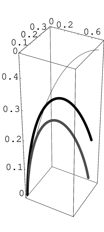
Figure 1: Trial (thin line), intermediate (thick line) and final (thick gray line) solutions for a rod with desired end point at ${\bf r}_{f}=(0.7,0.0)$. The load parameters are $P_{\psi}=1$, $P_{\phi}=1$ and $F=1$, in scaled units.

Figure 1 shows a example of the method. We have chosen the following load parameters in scaled units (see Eq. (11): $P_{\psi}=1.0$, $P_{\phi}=1.0$ and $F=1.0$. The desired end point is $r_{f}=0.7$ and $z_{f}=0.0$. We plot the trial, an intermediate and the converged rods together, in order to show the process of convergence from the trial to the desired solution. The trial solution was computed integrating the Kirchhoff equations starting from $\theta_{0}=0.5$ and $P_{\theta 0}=1.0$, which corresponds to a rod whose final point is $r_{f}\simeq 0.8$ and $z_{f}\simeq 0.455$. The intermediate solution was computed from $\theta_{0}\simeq 0.216$ and $P_{\theta 0}\simeq 2.257$, which corresponds to a rod whose final point is $r_{f}\simeq 0.73$ and $z_{f}\simeq 0.15$. Finally, the initial conditions obtained for the converged solution are $\theta_{0}\simeq 0.307$ and $P_{\theta 0}\simeq 2.510$.

V Numerical Examples

The particular trial solution used in the previous numerical example converged smoothly to the chosen final position. In some cases, however, a given trial solution does not converge to its destination no matter how many intermediate steps are used to divide the line between ${\bf r}_{t}$ and ${\bf r}_{f}$. As we shall see, this problem has to do with the existence or not of solutions for a given ${\bf r}_{f}$. In scaled units, it is obvious that there are no solutions if $\sqrt{r_{f}^{2}+z_{f}^{2}}>1$. The restrictions are actually much stronger than this simple ’length rule’, and depend on the values of $P_{\phi}$, $P_{\psi}$ and $F$. It might also happen that the solution for a given ${\bf r}_{f}$ does exist, but that the straight line connecting ${\bf r}_{t}$ to ${\bf r}_{f}$ passes through forbidden regions, hindering the convergence. In this section we investigate the space of possible solutions and give several examples of rods computed with our method.

Each initial condition $\theta_{0}$ and $P_{\theta 0}$ leads to an end point ${\bf r}_{f}$. The easiest way to map all possible final points is to scan the space of initial conditions. Therefore, for a fixed set of parameters $P_{\psi}$, $P_{\phi}$ and $F$ we calculate ${\bf r}_{f}={\bf r}_{f}(\theta_{0},P_{\theta 0})$ and plot the resulting figure in the $(r_{f},z_{f})$ space. Points outside this region are unreachable by the rod. Changing the parameters, such as the tension, changes the region of possible solutions, including end-points that were not previously present and excluding others.

The results in this section are presented as follows: for each fixed set of $P_{\psi}$, $P_{\phi}$ and $F$ we show the $(r_{f},z_{f})$-space of possible solutions. On the same plot we draw curves of constant $D=\sqrt{r_{f}^{2}+z_{f}^{2}}$ and, for each $D$ we compute the three dimensional configuration of a few rods.

In order to compare the rods, we always adjust the value of $\psi_{0}$ such that the rod ends in $y_{f}=0$ plane. $\psi_{0}$ is determined by:

$$\tan\psi_{0}=\frac{y_{f}^{0}}{x_{f}^{0}}$$ (51)

where $x_{f}^{0}$ and $y_{f}^{0}$ are the final values of $x$ and $y$ for the rod calculated with $\psi_{0}=0$.

In all cases tested our method converged with at least six significant figures to the previously defined final values of $r_{f}$ and $z_{f}$.

V.1 $P_{\psi}=0,P_{\phi}=1$ and $F=0.1$

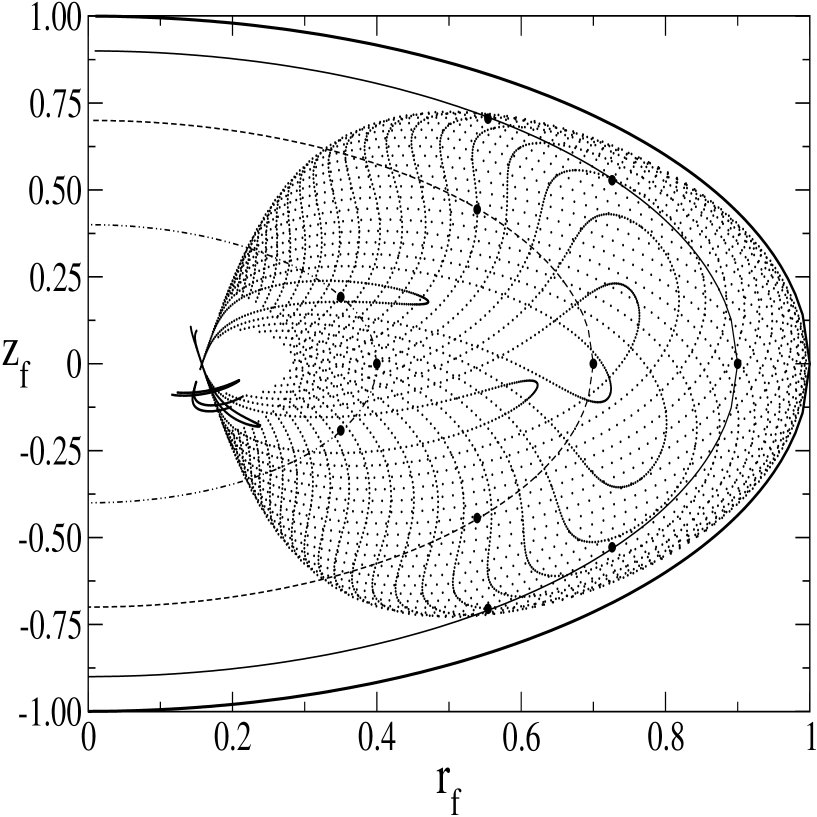
Figure 2: Regions of the existence of final points for $P_{\psi}=0$, $P_{\phi}=1$, $F=0.1$. The curves $D=1.0$ (full thick line), $D=0.9$ (full line), $D=0.7$ (dashed line) and $D=0.4$ (dotted-dashed line) are also shown. The circles correspond to the rods in the Figure 3.The plot was generated by varying the initial conditions in the intervals $0<\theta_{0}<\pi$ ($30$ points) and $-5.0<P_{\theta 0}<5.0$ ($200$ points).

Figure 2 shows the $(r_{f},z_{f})$ map for this case. The map was generated by varying the initial condition in the intervals $0<\theta_{0}<\pi$ ($30$ points) and $-5.0<P_{\theta 0}<5.0$ ($200$ points). For larger values of $P_{\theta 0}$ the total elastic energy of the rod increases and the final points tend to concentrate in the region near the origin (data not shown). The full thick line represents the curve $D=1.0$, which is the natural limit for the solutions. But there is a large region inside the $D=1$ line where no solutions exist. We shall compare it with that of other load parameters later on. We also show the lines of constant $D$ for $D=0.9$ (full line), $D=0.7$ (dashed line) and $D=0.4$ (dotted-dashed line). It is also interesting to note a forbidden region centered around $z_{f}\sim 0$ and $r_{f}\sim 0.25$. From the sequence of points crossing each other, it is evident that there are two sets of initial conditions $(\theta_{0},P_{\theta 0})$ that generate rods with the same end point. In general they correspond to rods that are above or below the $z$ axis, and we shall call them the ’up’ solution and the ’down’ solution respectively.

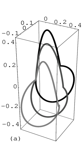
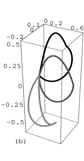
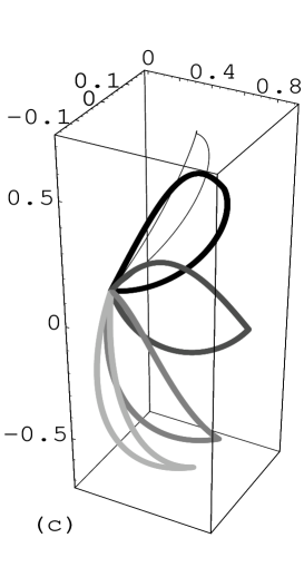
Figure 3: Up and down solutions (drawn in the same color) for the end points shown by the circles in Fig. 2. (a) $D=0.4$; (b) $D=0.7$; and (c) $D=0.9$.

Figure 3 shows examples of the rods whose end points are marked with circles in Fig. 2. We show the up and down solutions for each final point. Figs. 3a and 3b show three rods each for $D=0.4$ and $D=0.7$. Fig. 3c shows 5 different rods for $D=0.9$.

Notice that when $P_{\phi}$ or $P_{\psi}$ are zero, the hamiltonian (22), becomes symmetric under the transformation $F\rightarrow-F$ and $\theta\rightarrow\pi-\theta$. In these cases the ’up’ solution for a given $F$ and $\theta_{0}$ is identical to the ’down’ solution for $-F$ and $\pi-\theta_{0}$. When both $P_{\phi}$ and $P_{\psi}$ are non-zero the symmetry disappears.

V.2 $P_{\psi}=0,P_{\phi}=5$ and $F=1$

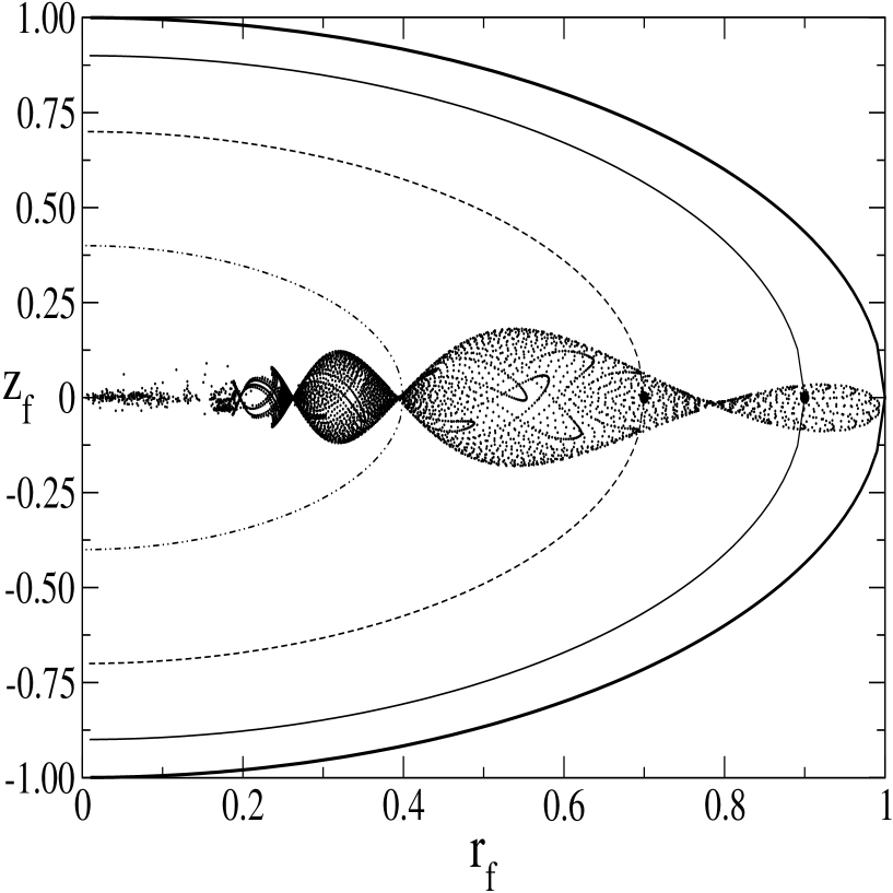
Figure 4: Regions of the existence of final points for $P_{\psi}=0$, $P_{\phi}=5$, $F=1$. The curves $D=1.0$ (full thick line), $D=0.9$ (full line), $D=0.7$ (dashed line) and $D=0.4$ (dotted-dashed line) are also shown. The circles indicate the rods drawn in Figure 5. The plot was generated by varying the initial conditions in the intervals $0<\theta_{0}<\pi$ ($30$ points) and $-20.0<P_{\theta 0}<20.0$ ($200$ points).

The $(r_{f},z_{f})$ map for these parameters is shown in Fig. 4. It has a curious pattern of thin bulbs centered around the $z_{f}=0$ axis, that degenerate for small $r_{f}$. The only rods possible in this case are those that return close to the $z=0$ plane.

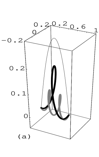
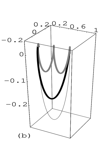
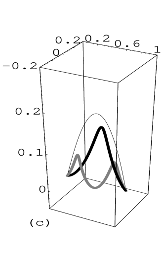
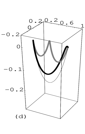
Figure 5: Rods for $P_{\psi}=0$ and $F=1$. The lines corresponds to $P_{\phi}=1$ (thin black), $P_{\phi}=5$ (thick black) and $P_{\phi}=10$ (gray). (a) up solutions for $r_{f}=0.7$; (b) down solutions for $r_{f}=0.7$; (c) up solutions for $r_{f}=0.9$; (d) down solutions for $r_{f}=0.9$.

Keeping $P_{\psi}=0$ and $F=1$ but increasing $P_{\phi}$ results in even thiner bulbs. Figures 5 (a) and (b) show the up and down solutions, respectively, for $r_{f}=0.7$, $z_{f}=0$ and $P_{\phi}=1$, $5$ and $10$. Panels (c) and (d) show the up and down solutions for the same parameters, except for $r_{f}=0.9$. Notice that large values of $P_{\phi}$ correspond to horizontal helical rods.

V.3 $P_{\psi}=P_{\phi}$ and $F=1$

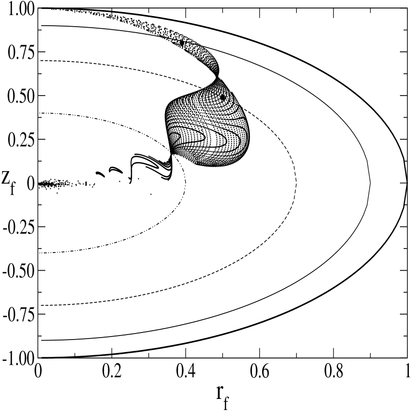
Figure 6: Regions of the existence of final points for $P_{\psi}=P_{\phi}=5$, $F=1$. The curves $D=1.0$ (full thick line), $D=0.9$ (full line), $D=0.7$ (dashed line) and $D=0.4$ (dotted-dashed line) are also shown. The circles indicate the rods drawn in Figure 7. The plot was generated by varying the initial conditions in the intervals $0<\theta_{0}<\pi$ ($30$ points) and $-10.0<P_{\theta 0}<10.0$ ($200$ points).

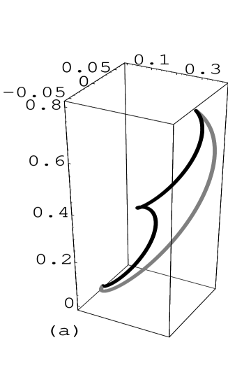
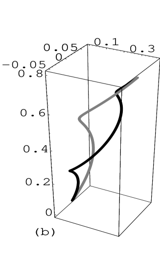
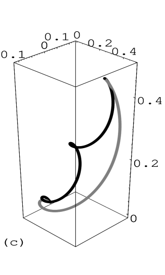
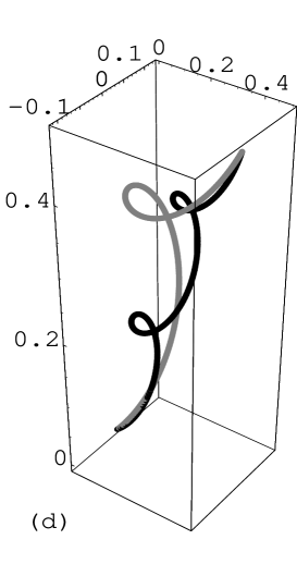
Figure 7: Rods for $P_{\psi}=P_{\phi}$ and $F=1$. The lines corresponds to $P_{\phi}=P_{\psi}=10$ (black) and $P_{\phi}=P_{\psi}=5$ (gray). (a) and (b) show the up and down solutions for $r_{f}=0.39$ and $z_{f}=0.8$; (c) and (d) show the up and down solutions for $r_{f}=0.5$ and $z_{f}=0.49$

Figure 6 shows the $(r_{f},z_{f})$ map for $P_{\psi}=P_{\phi}=5$. It resembles the map on Fig. 4, only distorted towards $z_{f}=1$. For these values of the parameters the rod admits ’vertical’ configurations, as opposed to the ’horizontal’ configurations displayed in the previous case. Figures 7 show examples of rods with $P_{\psi}=P_{\phi}=5$ and $P_{\psi}=P_{\phi}=10$ for $r_{f}=0.39$ and $r_{f}=0.5$.

VI Application to Non-homogeneous DNA

As a last application of our method we shall consider the equilibrium configurations of non-homogeneous rods. We restrict ourselves to the simplest case of periodic non-homogeneities in Young’s modulus. The motivation for this study is the fact that repeated (and therefore periodic) DNA sequences form a substantial fraction of all eukaryotic genomes jenny ; brian . The calculations presented here are based on the stiffness parameters recently computed for the 32 tri-nucleotide units from DNA data gromiha . Our goal is to understand how much the equilibrium configuration of a non-homogeneous rod differs from that of the homogeneous case when the rod is subject to fixed mechanical conditions.

Repetitive DNA is formed by nucleotide sequences of varying lengths and compositions. Repeated sequences, reaching up to 100 megabasepairs of length brian , appear to have little or no functional role, and are commonly regarded as “selfish” or “junk” DNA mclister . We shall use a simple periodic formula for the (scaled) Young’s modulus that covers most of the parameter interval spanned by the tri-nucleotides given in ref. gromiha :

$$E(s)=1+\alpha\cos\frac{2\pi}{{\cal L}}s\;.$$ (52)

${\cal L}$ is the period of the oscillations of the Young’s modulus along the DNA and $\alpha$ is a parameter that depends on the specific sequence being repeated and that can not be greater than $0.66$.

Eqs.(22)-(25) have to be slightly modified to include the non-constant Young’s and shear moduli. We obtain

$$H=\frac{P^{2}_{\theta}}{2E(s)}+\frac{P^{2}_{\phi}}{2\Gamma_{0}\mu(s)}+\frac{(P_{\psi}-P_{\phi}\cos\theta)^{2}}{2E(s)\sin^{2}\theta}+F\cos\theta,$$ (53)

with

$$P_{\theta}=E(s)\theta^{\prime},$$ (54)

$$P_{\phi}\equiv M_{3}=\Gamma_{0}\mu(s)(\phi^{\prime}+\psi^{\prime}\cos\theta),$$ (55)

$$P_{\psi}\equiv M_{Z}=E(s)\psi^{\prime}\sin^{2}\theta+P_{\phi}\cos\theta.$$ (56)

The solutions do not depend on $\mu(s)$, since it does not enter in the differential equations for $\theta$, $P_{\theta}$ and $\psi$. Notice that these equations are not integrable if $\alpha\neq 0$. Although $P_{\psi}$ and $P_{\phi}$ are still constants, the elastic energy per unit arclength is not.

The method for solving the BVP for a non-homogeneous rod is the following: consider a solution extending from the origin to ${\bf r}_{f}$ with $\alpha=0$ and initial conditions $\theta_{0}$ and $P_{\theta_{0}}$. Now integrate the Kirchhoff equations from the same initial conditions but using Eq.(52) with $\alpha\neq 0$. This new solution, whose end point is ${\bf r}_{f}+\delta{\bf r}$, can be used as a trial solution for the non-homogeneous rod. Using the method of section IV we push the rod back to ${\bf r}_{f}$.

Figure 8 shows the up and down solutions for load parameters $F=1$, $P_{\psi}=0$, $P_{\phi}=10$, $r_{f}=0.9$ and $z_{f}=0$ for the homogeneous rod (black curve) and a non-homogeneous rod with $\alpha=0.66$ and ${\cal L}=0.1$ (gray curve).

Finally, Figure 9 shows the effect of changing the period of oscillations in Young’s modulus. We show the up and down solutions for non-homogeneous rods with the same load parameters of the previous figure and $\alpha=0.66$. The curves show rods for ${\cal L}=0.1$ (gray), ${\cal L}=0.5$ (thick black) and ${\cal L}=0.65$ (thin black). The changes in the three-dimensional shape of the rods are evident for these values of load parameters. The sensitivity of the three-dimensional shape to the base-pair sequences indicated that DNA repeats may have conformational roles.

VII Conclusions

In this work we presented a general method to solve the boundary value problem (BVP) for finite Kirchhoff filaments. The method consists in making small changes to a known trial rod that satisfies the Kirchhoff equations but not necessarily the boundary conditions. We combine a shooting technique with the method of monodromy matrix to push the end point of the trial solution to the desired position, step by step. By linearizing the Kirchhoff equations we obtain an explicit relation between a variation of the initial conditions (expressed in terms of Euler angles) and the consequent variation of the rod’s end point.

The solutions of the BVP are limited by the physical constraints of the rod, such as the moments and tension. A sketch of the allowed end points can be constructed by integrating the Kirchhoff equations for a large number of initial conditions. The regions of possible end points form complex figures reflecting the non-linear character of the equations. The regions of existence of end points may serve as a guide to find the appropriate load parameters needed for a desired solution.

We presented several examples of rods with different end positions at different distances from the origin for various sets of load parameters. In all cases the method worked very well and the BVP was solved with at least six significant figures in the values of $r_{f}$ and $z_{f}$. We also applied the method to non-homogeneous, sequence-dependent, DNAs. We modeled pieces of repeated sequences by a sinusoidal oscillation of the Young’s modulus. We showed that the tri-dimensional structure of the DNA is indeed sensitive to the presence of such sequences, a property that has been considered before hogan but studied only in terms of the DNA intrinsic curvature manning . The effect studied here may contribute to other sequence-dependent properties that affect the three-dimensional conformations of the DNA.

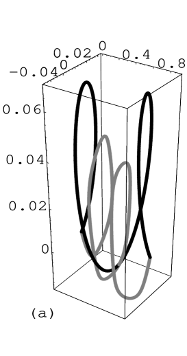
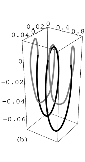
Figure 8: Comparison between homogeneous and non-homogeneous rods. Panels (a) and (b) show the up and down solutions respectively. The parameters are $P_{\psi}=0$, $P_{\phi}=10$, $F=1$, $r_{f}=0.9$ and $z_{f}=0$. The black curve shows the homogeneous rod and the gray curve the non-homogeneous rod with $\alpha=0.66$ and ${\cal L}=0.1$.

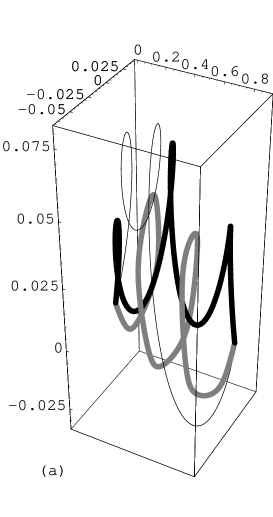
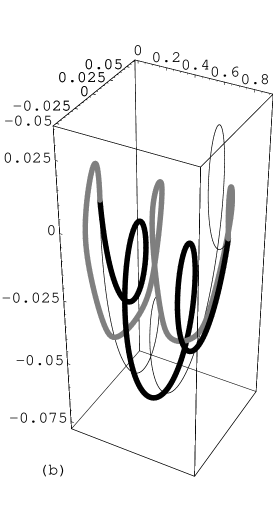
Figure 9: Comparison between non-homogeneous rods with different periods ${\cal L}$. Panels (a) and (b) show the up and down solutions respectively. The load parameters and final position $\mathbf{r}_{f}$ are the same as in Fig. 8. The curves show rods for ${\cal L}=0.1$ (gray), ${\cal L}=0.5$ (thick black) and ${\cal L}=0.65$ (thin black)

- (1) J. Coyne, IEE Journal of Oceanic Engineering 15, 72 (1990).
- (2) E. E. Zajac, Trans. ASME, 29, 136 (1962).
- (3) Y. Sun and J. W. Leonard, Ocean Engineering 25, 443 (1997).
- (4) M. A. Vaz and M. H. Patel, Appl. Ocean Res. 22, 45 (2000).
- (5) M. D. Barkley and B. H. Zimm, J. Chem. Phys. 70, 2991 (1979);
- (6) Y. Yang, I. Tobias and W. K. Olson, J. Chem. Phys. 98, 1673 (1993);
- (7) Y. Shi and J. E. Hearst, J. Chem. Phys. 101, 5186 (1994).
- (8) T. Schlick, Curr. Opin. Struct. Biol. 5, 245 (1995). W. K. Olson, Curr. Opin. Struct. Biol. 6, 242 (1996).
- (9) R. E. Goldstein and S. A. Langer, Phys. Rev. Lett. 75, 1094 (1995);
- (10) C. W. Wolgemuth, T. R. Powers and R. E. Goldstein, Phys. Rev. Lett. 84, 1623 (2000).
- (11) I. Klapper, J. Comput. Phys. 125, 325 (1996).
- (12) A. Goriely and M. Tabor, Phys. Rev. Lett. 80, 1564 (1998).
- (13) A. Goriely and T. McMillen, Phys. Rev. Lett. 88, art. no. 244301 (2002).
- (14) G. Kirchhoff, J. Reine Anglew. Math. 56, 285 (1859).
- (15) W. K. Olson and V. B. Zhurkin, Curr. Opin. Struct. Biol. 10, 286 (2000).
- (16) E. H. Dill, Arch. Hist. Exact. Sci. 44, 2 (1992); B. D. Coleman, E. H. Dill, M. Lembo, Z. Lu and I. Tobias , Arch Rational Mech. Anal. 121, 339 (1993).
- (17) M. Nizzete and A. Goriely, J. Math. Phys. 40, 2830 (1999).
- (18) A. Goriely and M. Tabor, Physica D 105 20 (1997); Physica D 105, 45 (1997).
- (19) A. Goriely and M. Tabor, Nonl. Dyn. 21, 101 (2000).
- (20) A. F. Fonseca and M. A. M. de Aguiar, Phys. Rev. E 63, art. n. 016611 (2001).
- (21) I. Tobias, D. Swigon and B. D. Coleman, Phys. Rev. E 61, 747 (2000); B. D. Coleman, D. Swigon and I. Tobias, Phys. Rev. E 61, 759 (2000).
- (22) I. Tobias, B. D. Coleman and W. K. Olson, J. Chem. Phys. 101, 10990 (1994).
- (23) A. Balaeff, L. Mahadevan and K. Schulten, Phys. Rev. Lett. 83, 4900 (1999).
- (24) M. Baranger and K. T. R. Davis, Ann. Phys. (N.Y.) 177, 330 (1987).
- (25) A.L. Xavier Jr. and M. A. M. de Aguiar, Ann. Phys. (N.Y.) 252, 458 (1996).
- (26) H. B. Keller, Numerical Solution of Two Point Boundary Value Problems (Capital City Press, Montpelier, 1990).
- (27) S. N. Ha, Int. J. Comp. and Math. 42, 1411 (2001).
- (28) A. R. Champneys and A. Spence, Adv. Comp. Math. 1, 81 (1993).
- (29) T. McMillen and A. Goriely, J. Nonlinear Science 12, 241 (2002).
- (30) A. R. Champneys, G. H. M. van der Heijden and J. M. T. Thompson, Phil. Trans. R. Soc. Lond. A 355, 2151 (1997).
- (31) G. H. M. van der Heijden, A. R. Champneys and J. M. T. Thompson, SIAM J. App. Math. 59, 198 (1997).
- (32) G. Károlyi and G. Domokos, Physica D 134, 316 (1999).
- (33) O. Gottlieb and N. C. Perkins, ASME J. Appl. Mech. 66, 352 (1999).
- (34) G. J. L. Wuite, R. J. Davenport, A Rappaport and C. Bustamante, Biophys. J. 79, 1155 (2000).
- (35) J. C. Meiners and S. R. Quale, Phys. Rev. Lett. 84, 5014 (2000).
- (36) A. Bensimon, A. Simon, A. Chiffaudel, V. Croquette, F. Heslot and D. Bensimon, Science 265, 2096 (1994).
- (37) R. Schleif, Annu. Rev. Biochem. 61, 199 (1992).
- (38) A. Balaeff, L. Mahadevan and K. Schulten, Phys. Rev. Lett. 83, 4900 (1999).
- (39) J. Hsieh and A. Fire, Annu. Rev. Genet. 34, 187 (2000).
- (40) B. Charlesworth, P. Sniegowski and W. Stephan, Nature 371, 215 (1994).
- (41) M. M. Gromiha, J. Biol. Phys. 26, 43 (2000).
- (42) B. F. McAllister and J. H. Werren, J. Mol. Evol. 48, 469 (1999).
- (43) M. E. Hogan and R. H. Austin, Nature (London) 329, 263 (1987).
- (44) R. S. Manning, J. H. Maddocks and J. D. Kahn, J. Chem. Phys. 105, 5626 (1996).