A stochastic model for heart rate fluctuations

Abstract

Normal human heart rate shows complex fluctuations in time, which is natural, since heart rate is controlled by a large number of different feedback control loops. These unpredictable fluctuations have been shown to display fractal dynamics, long-term correlations, and 1/f noise. These characterizations are statistical and they have been widely studied and used, but much less is known about the detailed time evolution (dynamics) of the heart rate control mechanism. Here we show that a simple one-dimensional Langevin-type stochastic difference equation can accurately model the heart rate fluctuations in a time scale from minutes to hours. The model consists of a deterministic nonlinear part and a stochastic part typical to Gaussian noise, and both parts can be directly determined from the measured heart rate data. Studies of 27 healthy subjects reveal that in most cases the deterministic part has a form typically seen in bistable systems: there are two stable fixed points and one unstable one.

I Introduction

Various methods and models have been used in attempts to characterize the dynamics of the heart rate control mechanism. For short time periods and under stationary conditions there are successful models of heart rate and blood pressure regulation Seidel (1998); ten Voorde (1992), but the characterization of long-term behavior has been a very difficult problem. Some models have been introduced in order to explain long-term fluctuations, but usually they can only describe well-controlled in vitro experiments, or the models depend on large number of parameters, which cannot be easily determined from experimental data Glass and Mackey (1988). Furthermore, these models can predict only global statistical features like scaling properties of power spectrum and correlations Ivanov et al. (1998) and tell us very little about the details of the time evolution.

Many features can be extracted from long time series of heart rate measurements, quantities like entropy measures Bettermann and van Leeuwen (1998); Kaspar and Schuster (1987); Pincus and Goldberger (1995); Pincus (1995); Rezek and Roberts (1998); Richman and Moorman (2000); Zhang and Roy (1999) correlation dimension Farmer et al. (1983); Fell et al. (1996); Grassberger and Procaccia (1983); Kantz and Schreiber (1995); Mayer-Kress et al. (1988); Yum et al. (1999), detrended fluctuations Peng et al. (1993, 1995); Iyengar et al. (1996), fractal dimensions Bassingthwaighte and Raymond (1995); Chau et al. (1993); Gough (1993); Zhang and Roy (1999), spectrum power-law exponents Bigger et al. (1996); Iyengar et al. (1996)) and symbolic dynamics complexity Palazzolo et al. (1998); Voss et al. (1995, 1996), but these are all purely statistical characterizations and as such cannot provide us a mathematical model of heart rate dynamics, not even a simple one. However, some of these statistical methods do characterize the complexity of the dynamics underlying the time series Kuusela et al. (2002), or are directly related to their fractal or chaotic features. Mathematical analysis of many physiological rhythms, including long-term heart rate fluctuations, has revealed that they are generated by processes which must be nonlinear, since linear systems can not produce such a complex behaviour Glass (2001). Nonlinear purely deterministic models can display chaotic dynamics and generate apparently unpredictable oscillations, but in practice it has not yet been possible to extract such models from real noisy experimental data. It is also possible that the underlying system is stochastic, i.e., the time evolution of the system is subject to a noise source. [This kind of dynamical noise is different from measurement noise, which is mostly generated in the experimental apparatus.] In any case, there is increasing evidence that noise, originated either from the system itself or as a reflection of external influences, is actually an integral part of the dynamics of biological systems Collins et al. (1996); Hidaka et al. (2000); Mar et al. (1999).

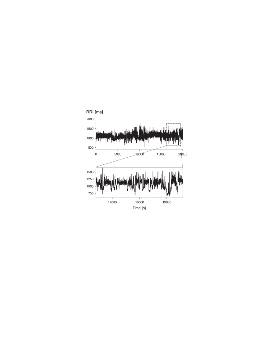
Figure 1: Typical R-R interval time series recorded at night

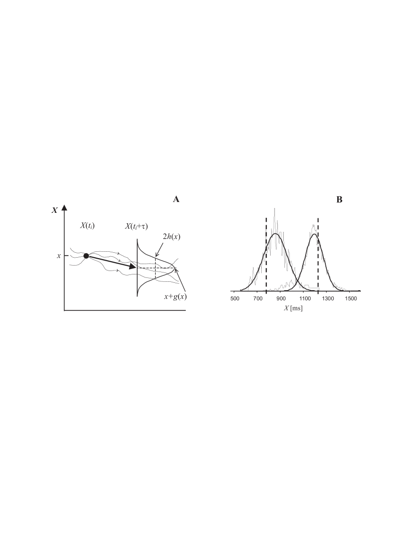
Figure 2: Schematic presentation of the method for analyzing stochastic time series and calculating the deterministic and stochastic part of the dynamics (Fig. A). Whenever the trajectory of the system passes near certain point $x$ in the state phase, i.e. $X(t_{i})\approx x$, the future value $X(t_{i}+\tau)$ of the trajectory is recorded. The distribution of these values is fitted by a Gaussian function with the mean $x+g(x)$ and deviation $h(x)$, cf. equation (2). This is repeated for all $x$-values. On the right are two typical examples of the distribution of future values, the initial $x$ values are marked with dashed vertical bars and the fitted Gaussian curves with a thick line (Fig. B).

A typical R-R interval recording is shown in Fig. 1. The time series is generated by recording a 24-hour electrocardiogram and detecting the R-peak from each heartbeat, the R-R interval is the time difference between two consecutive R-peaks. In the upper panel of Fig. 1 we have the R-R interval time series for 6 hours. We can see sections where the oscillations are rather regular but there are also abrupt changes. In the lower panel of Fig. 1 we have zoomed into a part of the time series, about $50$ minutes, and also on this time range we can see apparently random oscillations with rapid changes.

It is well known that most short-time fluctuations of heart-rate are generated by respiration (periods typically in the couple of seconds range) and blood pressure regulation (so called Meyer waves with periods of about 10 seconds Guyton and Hall (1996)). In the following we are not interested in these fast rhythms (which can be analyzed quite well using linear or semi-linear models) but rather in time scales from minutes to hours. We will show that in this time range the dynamics of the heart-rate fluctuations can be well described by a one-dimensional Langevin type difference equation. This equation contains a deterministic part and additive Gaussian noise, and we have found that it works well when the delay parameter in the equation is in the range of 2–20 minutes.

II The Model

An important and wide class of dynamic systems can be described by the Langevin differential equation van Kampen (1981); Risken (1984)

$$\dfrac{dX(t)}{dt}=g(X(t),t)+h(X(t),t)\Gamma(t).$$ (1)

Here $X(t)$ represent the state of the system at time $t$, the function $g$ gives the nonlinear deterministic change, and the last term $h$ is the amplitude of the stochastic contribution and $\Gamma(t)$ stands for uncorrelated white noise with vanishing mean. These kinds of stochastic differential equations always need an interpretation rule for the noise term, normally one uses the Ito interpretation Ito (1950). In general the functions $g$ and $h$ could depend explicitly on time $t$. The equation (1) can be easily generalized to higher dimensions. We will now show that long-term behaviour of heart rate can be modeled using a difference version of the Langevin equation van Kampen (1981)

$$X(t+\tau)=X(t)+g(X(t);\tau)+h(X(t);\tau)\Gamma(t).$$ (2)

Here $X(t)$ again represents the state of the system, in this case the R-R interval, at time $t$, and $\tau$ is the time delay. If arbitrary small delays $\tau$ are possible then one can take the limit $\tau\rightarrow 0$ and get the differential equation (1) [if the $\tau$ dependence is given by $g(X(t);\tau)\approx\tau g(X(t))$], but in the present case it will turn out that there is a minimum $\tau$ for which the model (2) seems to be valid. We assume that $g$ and $h$ do not have explicit time dependence but they may depend on the delay $\tau$. It is convenient to extract the term $X(t)$ in the deterministic part, as is done in (2), then a nonzero $g(X(t);\tau)$ stands for changes in the state of the system. An essential feature of models of the above type is that for time evolution we only need to know the state at one given moment and not its evolution in the past, i.e., they are Markovian Hänggi and Thomas (1982); van Kampen (1981).

The computational problem is now to determine the functions $g$ and $h$ from measured time series and to verify that the description using (2) is accurate. The principle of the method is very simple Gradišek et al. (2000); Siegert et al. (1998): at every time $t_{i}$ when the trajectory of the system meets an arbitrary but fixed point $x$ in state space, we look at the future state of the system at time $t_{i}+\tau$. The set of these future values (for a chosen $x$ and $\tau$) has a distribution in the state space and from this distribution we can determine the deterministic part $g(x)$ and the stochastic part $h(x)$, see Fig. 2A. In practice we first divide the range of the dynamical variable $X$ into equal boxes. By scanning the whole measured time series we check when $X$ is inside a given box $x$, i.e., $|X(t_{i})-x|\leq\Delta x$ , where $x$ is the middle value of the box and $\Delta x$ is the half width of the box. When $X$ is found on the box, we look at the future value of the variable, $X(t_{i}+\tau)$, where $\tau$ is the fixed delay parameter. Since the trajectory of the system passes each box several times, we can calculate the distribution of the future values $X(t_{i}+\tau)$ for each box $x$. If we assume that the noise is Gaussian, we can fit a Gaussian function on each distribution, and as a result we get the mean and the deviation parameters for each $x$; the mean of this distribution is equal to $x+g(x)$ and the deviation is equal to $h(x)$ Friedrich et al. (2000); Timmer (2000). A typical case is given in Fig. 2B, and it shows that the distribution is actually very well described by Gaussian noise (the correlation is better than 0.95; the correlation is calculated as $\sqrt{1-S_{res}/{S_{tot}}}$, where $S_{res}$ is the sum of the squared residuals and $S_{tot}$ is the variance). From the given data we can in this way determine the functions $g(X)$ and $h(X)$ needed in the stochastic model (2). It should be noted that we can calculate only the absolute value of $h(X)$ since the deviation parameter found from the fitted Gaussian function is in squared form.

In our analysis we have used R-R interval time series of $22$–$24$ hours, corresponding to $80.000$–$100.000$ data points. Our data is actually interval data, i.e., it consists of a sequence of R-R interval values. It is then convenient to count the delay in our analysis in terms of heart-beats rather than seconds, i.e., we have not used cumulative time as time variable but the beat index. However, since the R-R interval values vary a lot within the used delay range, the beat index actually gives a delay as if computed with the average beat-rate. We have tested both methods and found only minor differences between them (in the details of the functions $g$ and $h$). We will show later that the functional forms of $g$ and $h$ are quite insensitive on the time delay, and since this holds for both methods we will use the more convenient beat index.

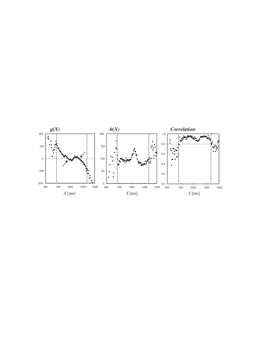
Figure 3: Typical results derived from R-R interval time series using time delay $\tau=500$. We have shown the deterministic part $g(X$) (the left panel), the stochastic part $h(X)$ (the middle panel) and the correlation coefficient of the distribution (the right panel) as a function of the dynamical variable $X$. The range corresponding to the correlation threshold level of $0.8$ is marked with the vertical lines.

III Results

III.1 A typical case

In Fig. 3 we have presented results obtained for a particular case using the method described earlier. The value of the delay parameter $\tau$ was $500$ beats, and the number of boxes used to construct local distributions was $150$. Distributions were fitted using Gaussian function. The $g(X$) function, the deterministic part of the system, is displayed on the left panel in Fig 3. It has a very clear and simple functional form (between the vertical lines) which is typical for systems exhibiting bistable behaviour Bergé et al. (1986); van Kampen (1981). The function crosses the zero line three times, these crossings are the fixed points of the system. The fixed points marked with arrows are stable: without any noise term these points attract all nearby states, because the control function $g(X)$ is locally decreasing. The middle fixed point is repulsive. Due to the stochastic part the system has a tendency to jump between the stable points if the amplitude of the noise is high enough. Far away from the stable points $g(X)$ increases or decreases strongly forcing the system rapidly back to oscillate around the stable points. The amplitude of the stochastic part of the system, function $h(X)$, is almost constant except between the stable points where it has a clear maximum (the middle panel in Fig. 3). One interpretation is that the system has a larger inherent freedom to oscillate randomly when the trajectory is between the stable points but outside this range the character of the system is more deterministic. From the physiological point of view this kind of dynamics can be useful since it lets the R-R interval to wander most of the time but prevents it from escaping too far away from the normal range. On the right panel in Fig. 3 we have shown the correlation coefficient of each local distribution. Most of the time the correlation is remarkably high, about $0.85$–$0.95$, but near the largest and smallest $X$ values there are only rather few data points and therefore the corresponding distributions do not have clear Gaussian shape resulting with lower correlation. The high average correlation value is a clear indication that the noise in this system is really Gaussian type. We have used the value of $0.8$ as a threshold level, and the corresponding range is marked with the vertical lines in Fig. 3.

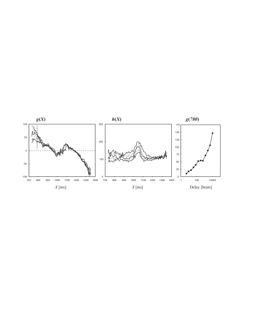
Figure 4: Examples of the deterministic part $g(X$) (the left panel) and the stochastic part $h(X$) (middle panel) calculated with various values of the delay parameter $\tau$ : $40$ (thick line), $80$ (thin line), $160$ (thick line), $320$ (thin line) and $640$ (thick line). The values of the $g(X$) function at $X=780$ ms (marked with vertical dashed line in the left panel) are plotted as a function of the delay in the right panel, there is a plateau around a delay of $100$–$1000$ beats.

What is remarkable in this description is that the functional forms of $g(X)$ and $h(X)$ are fairly independent of the delay parameter $\tau$ in a rather extensive delay range, typically $100$–$1000$ beats (corresponding to $2$–$20$ minutes). In Fig. 4 we have plotted the functions $g(X)$ and $h(X)$ for a range of $\tau$ values. The $g$-function is practically $\tau$ independent, except for the shortest R-R intervals, where some cumulative effects show up. The $h$-function seems to grow very slowly as $\tau$ increases. For still smaller delay values $g(X)$ is more flat and $h(X)$ is more scattered, and for longer delays $g(X)$ is typically a straight line and $h(X)$ is constant. Behavior at these extremes can be easily understood by recalling that when the time scale is small, the heart rate system is clearly multidimensional depending directly on blood pressure, respiration and other rapidly changing physiological variables and our 1-dimensional description is no longer valid. On the other hand, if the delay parameter is very large, we cannot reconstruct the local dynamics in terms of local distributions, we just get the global distribution that is independent of dynamics and no longer Gaussian. In the right panel of Fig. 4 we have given the values of the $g(X)$ function at $X=780$ ms (marked with a vertical dashed line in the left panel) computed with delays of $5$–$10240$ beats. We can see a plateau in the delay range of $100$–$1000$ beats which means that the $g(X)$ curves for these delays are bundled. In principle the curves for a delay of $2\tau$ should be obtainable by iterating (2) with delay $\tau$. Direct numerical calculations of joint probabilities using experimentally determined $g(X)$ (within $100$–$1000$ beats delay range) indicate that $g(X)$ and $h(X)$ do not change significantly in one iteration, mostly because in our case the Gaussian distribution is not so narrow. In general iterations tend to sharpen the bends in $g(X)$ and this feature is indeed visible in Fig. 4. The small $\tau$-dependency of $g$ and $h$ in the range of short R-R intervals can then be interpreted either as the expected result from repeated iterations, or as a sign of higher order dynamics: possibly the heart rate regulation system is more complex when the system must readjust at a fast heart rate.

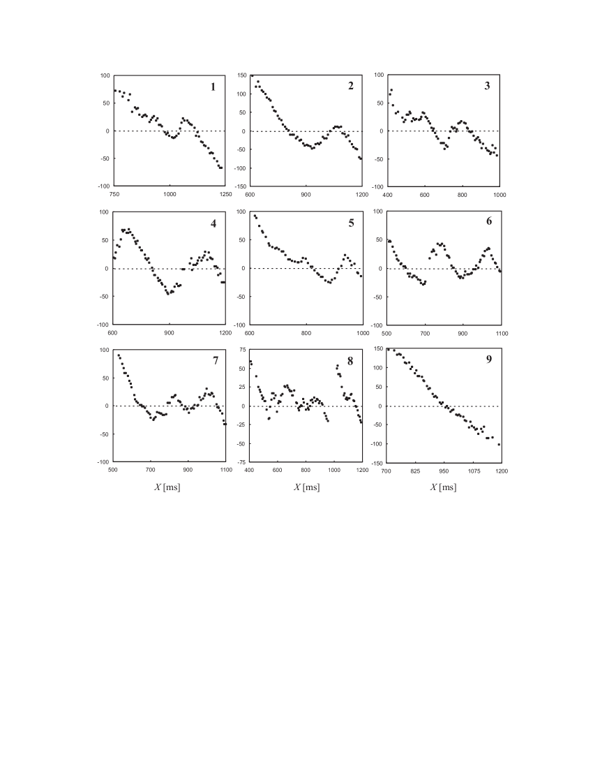
Figure 5: Typical deterministic functions $g(X)$ derived from different subjects. The cases 1 - 5 represent simple bistable situation, the cases 6 and 7 have three stable points, the case 8 is multistable, and the case 9 has only a single stable fixed point.

III.2 Variation between subjects

In order to find whether different subjects have are any common features in the deterministic and stochastic parts $g(X)$ and $h(X)$ we analyzed the data from $27$ healthy subjects of various age and gender [$18$ cases from PhysioBank Goldberger et al. (2000) and $9$ cases from Kuopio University Hospital]. Analyses were done using the same parameter values as in Fig. 3. The deterministic part, the $g(X)$ function, is displayed in Fig. 5 for a set of $9$ typical cases. The most common form for this function is the bistable type, already shown in Fig. 3, where the $g(X)$ function has three zeroes, and $60$% of all cases can be classified to this group (cases 1–5 in Fig. 5). The next most common group, $25$% of all cases, has a $g(X)$ function with $5$ zeroes, a kind of double pitchfork system (cases 6 and 7 in Fig. 5). We also found $3$ cases where the $g(X)$ function seems to have even more zeroes (case 8 in Fig. 5). Only very few cases could not be clearly classified as bi- or multistable. In these cases it can be difficult to interpret the results. It is possible that the dynamical variable did not explore the whole state phase, and therefore we can see only part of the $g(X)$ function; for example case 9 in Fig. 5, where the system has only one stable fixed point and no unstable points at all, can be an example of this. The stochastic parts (function $h(X)$) are fairly similar: they are almost constant except that in all cases there are maxima on the R-R interval ranges between the stable fixed points of the deterministic part, as in the example in Fig. 3.

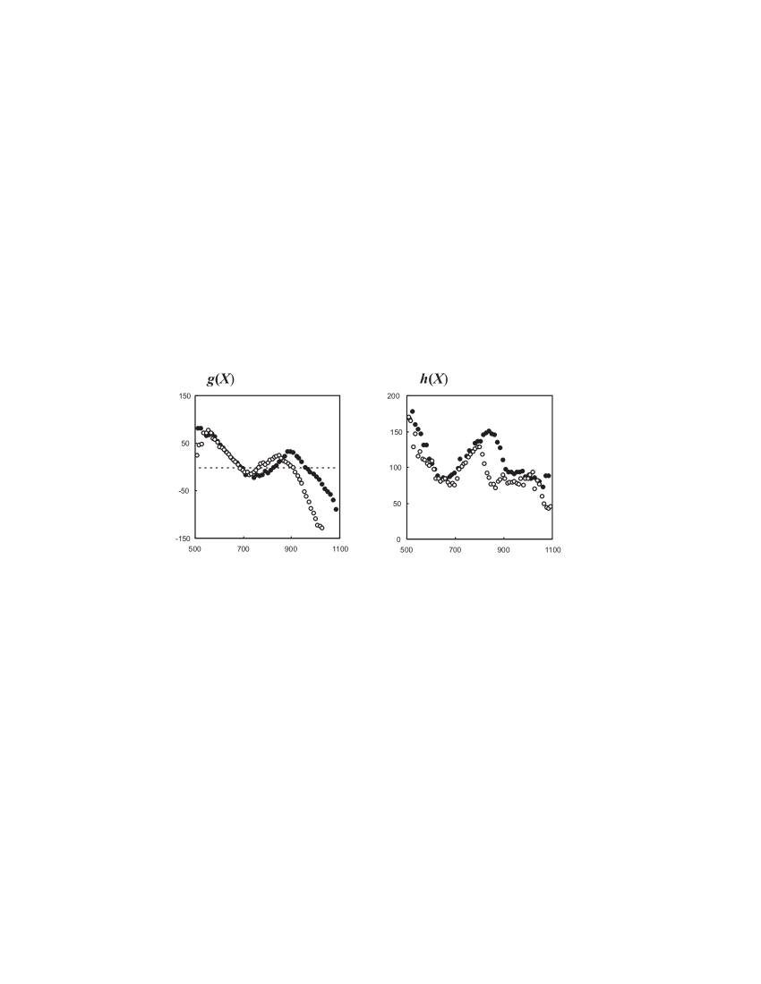
Figure 6: The deterministic parts $g(X)$ (left panel) and stochastic parts $h(X)$ (right panel) computed from the R-R interval time series recorded from the same subject on different days. The data from the first recording is marked with solid dots and data from the second recording, 4 days later, with open dots.

The description given by equation (2) contains both a deterministic and a stochastic component. It is an important to realize that the stochastic part is not a small perturbation but in fact forms an essential part of the description, furthermore it is $10$–$20$ times higher than the measurement noise (uncertainty in detecting the position of the R-peak), which is typically only $2$–$5$ ms. One way to compare the deterministic and stochastic components is to note that the size of the bend in the $g(X)$ function is of the order of $30$ to $50$ ms, while the average size of the $h(X)$ function is about $70$ to $110$ ms, as can be seen in Fig. 3. [The extraction of small details in the $g(X)$ function under such noise is of course possible only because the noise is so cleanly Gaussian.] On the other hand, the distance between the stable fixed points in the $g(X)$ function is of the order of $50$ to $250$ ms, and therefore the probability that the systems jumps between stable points is not extremely high, but nevertheless possible. It is also possible that external factors drive the system from one stable point to another, since during night-time the mean R-R interval is typically longer than during day-time [although the R-R interval can abruptly jump to the faster rate also during the night, as can be seen on the lower panel in Fig. 1].

III.3 Same subject at different times

If the model (2) were to describe true heart rate dynamics, the functions $g(X)$ and $h(X)$ should have some constant features specific for each subject. In order to look at this aspect we made two recordings from the same subject within 4 days, the results are shown in Fig. 6. In general the deterministic and stochastic parts from different recordings are remarkably similar both having clear bistable character. In the R-R interval range of $500$–$800$ ms the results are almost identical and the only difference seems to be a scaling towards the shorter R-R intervals in the $800$–$1100$ ms range of the second recording. In the first recording the mean value of R-R interval calculated over the 24 hour period was $781$ ms and in the second one $726$ ms. Therefore in the second recording the shortest R-R intervals are significantly more frequent and this can affect on the analysis results. These deviations could also reflect true changes on the underlying control system: it is well know that there are daily variations on functions of the autonomic nervous system.

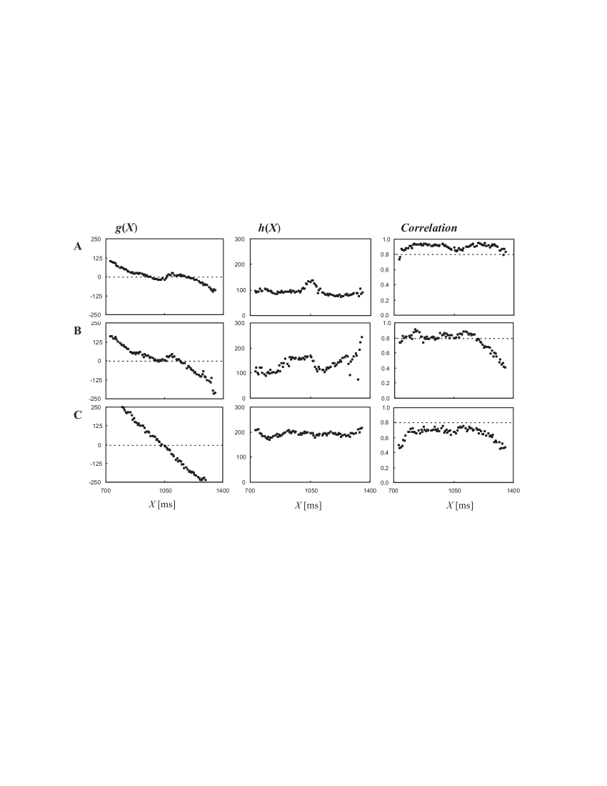
Figure 7: The deterministic part $g(X)$ (left column), stochastic part $h(X)$ (middle column) and correlation coefficient (right column) for the original data (row A) and for two surrogate versions (B and C). For surrogate data the original data has been shuffled using section sizes of $800$ (B) and $400$ (C) data points.

III.4 Surrogate analysis

As a further validity check we also performed surrogate analysis Schreiber and Schmitz (2000); Theiler et al. (1992) in order to eliminate the possibility that the results are generated just from peculiar distribution of the R-R intervals imitating real dynamics. For this purpose the data was shuffled by dividing it into sections of equal size which were then repositioned randomly. As a result we get a new time series where the dynamical structure has been partially destroyed depending on the section size. Results of this surrogate analysis are shown in Fig. 7. The top panels display the deterministic $g(X)$ and stochastic $h(X)$ parts of the system and the correlation coefficient without any data shuffling (row A in Fig. 7). On the next row (row B in Fig. 7) we have used sections of $800$ data points for shuffling. There are only small changes in the deterministic part, but the correlation has decreased noticeably. When the section size is $400$ (row C in Fig. 7) we can no longer see the bistable character in the deterministic part, the stochastic part is flat with higher mean level, and the average level of the correlation coefficient has dropped well below our threshold value $0.8$. With still smaller section sizes the results do not change any further. In this analysis we have used the same delay of $500$ data points as previously and when the section size used in the shuffling process is less than this delay all dynamical properties disappear, as expected in the case of true time evolution. Therefore we conclude that our results are derived from the dynamical properties of the heart beat data, and not from their overall statistical characteristics.

IV Conclusion

Our results indicate that the human heart-rate control dynamics can be accurately modeled with the 1-dimensional stochastic difference equation (2), where the time delay parameter is within $2$–$20$ minutes. Stochasticity is an integral part of the dynamics, and in this delay range the effects of other variables are either embedded into the stochastic part of the system or averaged over time with no net effect. It is remarkable that the form of the control function $g(X)$ is similar from case to case. Their typically bistable character is also well justified on common physiological grounds. From this initial study we cannot yet identify what kind of dynamical structure is typical for healthy subjects (although our results already indicate that a simple bistable system is most common feature) and therefore the model cannot yet be used directly for clinical work, for that purpose one needs extensive demographic studies. We can nevertheless speculate that the form of the control function $g(X)$ should tell us something about the health of the subject. Also, some of the current knowledge based on statistical measures of heart rate time series can probably be explained within the framework of our model. Another interesting observation is the importance of the stochastic part, it could be the result of integrating the effects of a more detailed control mechanism over time, but it could also reflect some truly stochastic internal and external influences.