An accelerator mode based technique for studying quantum chaos

Abstract

We experimentally demonstrate a method for selecting small regions of phase space for kicked rotor quantum chaos experiments with cold atoms. Our technique uses quantum accelerator modes to selectively accelerate atomic wavepackets with localized spatial and momentum distributions. The potential used to create the accelerator mode and subsequently realize the kicked rotor system is formed by a set of off-resonant standing wave light pulses. We also propose a method for testing whether a selected region of phase space exhibits chaotic or regular behavior using a Ramsey type separated field experiment.

Chaos in quantum mechanics is still a relatively poorly defined concept. Typically it is taken to refer to the behavior of a quantum system which in the classical limit exhibits an exponential sensitivity to initial conditions. A much studied example of such a system is the delta-kicked rotor Lichtenberg and Lieberman ; Casati . A realization of its quantum version, in the guise of cold atoms exposed to the ac-Stark shift potential of an off-resonant standing wave of light Raizen 1st QDKR , has elucidated many of the concepts associated with quantum chaos ResonancePRL ; Tunnelling2 ; Quantum-Classical ; Multi-dimensions . However, one substantial problem remains: there is no clear way of distinguishing regular from chaotic dynamics. In the quantum regime it is not possible to define a chaotic region of phase space as being one in which two initially similar states have an overlap which decreases exponentially with time. The unitary nature of any interaction necessarily implies that the overlap between such states remains unchanged. It has been suggested by Peres Peres that an alternative definition is needed for quantum systems. Peres’ proposal involves examining the evolution of a state which can interact with two potentials which differ very slightly in form. If the overlap between states produced by an evolution under each potential decreases exponentially as a function of time, then the region of phase space occupied by the initial state can be said to be chaotic in the quantum sense. The justification for this definition is that perturbation theory only converges when the region under examination has regular properties Feingold . More recently Gardiner et al. Gardiner97 have proposed an experiment with a trapped ion which would implement the essential features of Peres’ idea.

In this paper we address two problems related to the experimental determination of a phase space stability map for the atom optical version of the QDKR. Firstly, we demonstrate a method for preparing cesium atoms in a restricted region of phase space using the same standing wave light pulses which create the rotor. Secondly, we show how by examining the overlap between the wavefunctions of the two hyperfine levels of the $6^{2}S_{1/2}$ cesium ground state it should be possible to test the type of dynamics exhibited by the prepared atoms.

The basis of our atom optical version of the QDKR is exposure of laser cooled cesium atoms to pulses (duration $t_{{\rm p}}$ and separation time $T$) of a standing wave of off-resonant light. The pulses are short enough to allow the effect of the atoms’s kinetic energy to be neglected during a pulse. This places our experiment in the Raman-Nath regime in which the spatially periodic ac-Stark shift potential created by the light acts as a thin phase grating for the atoms AccModePRL . Thus an incident plane de Broglie wave is diffracted into a series of  “orders” separated in momentum by $\hbar G$, where $G=2k_{{\rm L}}$ ($k_{{\rm L}}$ is the light wavevector). One of the striking features of this system is the existence of quantum resonances ResonancePRL ; newfishman . These resonances occur when the pulse interval is a multiple of the half-Talbot time, $T_{\frac{1}{2}}=2\pi m/\hbar G^{2}$. During these special times all of the diffraction orders formed from incident plane waves with certain momenta will freely evolve phases which are multiples of $2\pi$. For cesium, the first quantum resonance occurs at $T=67$ $\mu$s.

In addition to being a paradigm of experimental quantum chaos, this system can also produce quantum accelerator modes AccModePRL . This is achieved by adding a potential of the form $U_{{\rm A}}(x)=max$, where $m$ is the atomic mass, $a$ is an applied acceleration and $x$ is the position along the standing wave. In our experiment the standing wave is oriented in the vertical direction, so $a$ is the acceleration due to gravity. Quantum accelerator modes are characterized by a fixed momentum transfer of (on average) $\xi\hbar G$ during each standing wave pulse (see Fig. 1 of Ref. AccModePRL ). Typically the accelerator modes are formed when the value of $T$ is near to a quantum resonance. For simplicity, we will henceforth confine our attention to pulse repetition times near to the first quantum resonance. One way of modelling the accelerator modes is to make the approximation that they consist of just a few diffraction orders (say $q-1$, $q$ and $q+1$, where $q$ is an integer) which in the time between two light pulses accumulate a phase difference which is very close to an integer multiple of $2\pi$. At the next pulse this makes it possible for interference to occur between the diffraction orders in such a way that the population of the three orders centered on $q+\xi$ non-integer am is enhanced. By using this rephasing condition, it can be shown AccModePRA  that after $N_{{\rm p}}$ pulses the central momentum of the accelerator mode is given by $q=\frac{N_{{\rm p}}}{\gamma}\frac{\alpha^{2}}{1-\alpha}=N_{{\rm p}}\xi$, where $\gamma=\hbar^{2}G^{3}/2\pi m^{2}a$ and $\alpha=T/T_{\frac{1}{2}}$. The same rephasing condition also leads to the conclusion that only incident plane waves with momenta

$$p_{{\rm init}}=\left(\alpha^{-1}l+{\rm const}\right)\hbar G$$ (1)

(where $l$ is any integer) can ever participate in an accelerator mode. Thus in momentum space an accelerator mode resembles a comb with a tooth spacing of $\alpha^{-1}\hbar G$. Furthermore, since plane waves separated by this momentum behave identically under the action of the kicks, the accelerator mode effectively contains only a single momentum. Figure 1(a) shows the theoretical momentum distribution of the accelerator mode after one set of pulses, as calculated using a model based on diffraction AccModePRL . To reflect the experimental situation the starting distribution was gaussian with a width of 12 $\hbar k_{\rm{L}}$ at FWHM. Although there is good qualitative agreement between Eq. (1) and the numerically derived momentum distribution, an explanation for the finite widths of the comb elements is needed. To understand this effect recall that each comb element must give rise to a set of diffraction orders which are always spaced by exact multiples of $\hbar G$. To determine what the real momentum distribution looks like we must add together the diffraction from all the different comb elements. These have a spacing of $\alpha^{-1}\hbar G$, which for pulse interval times just less than the Talbot time is slightly greater than $\hbar G$. The most obvious effect of including the diffraction orders is that the width of each comb element of the resultant distribution becomes non-zero and increases with $|\alpha-1|$. Additionally, when all the diffraction orders are weighted by the intensity of the comb element from which they originated, the nearest-neighbor spacing of the peaks in the momentum distribution is reduced as one moves away from the center of the distribution. The opposite effect is produced when the pulse interval is slightly greater than the Talbot time. Although the change in spacing is not immediately obvious in Fig. 1(a), it has been confirmed in a detailed analysis of this data.

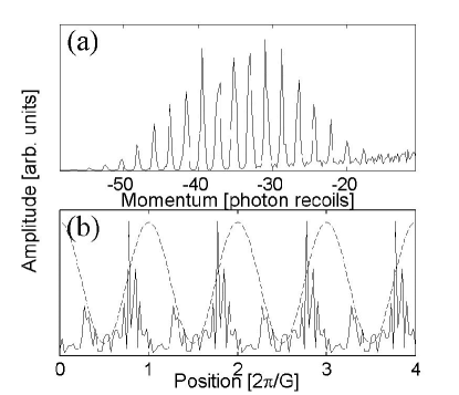
Figure 1: Numerically simulated momentum (a) and spatial (b) distributions of the accelerated component of an ensemble of cold cesium atoms after 20 pulses of an off-resonant standing light wave. The pulses had a separation of 60 $\mu$s. The momentum distribution consists of a comb of peaks separated by a little more than two photon recoils. The degree of spatial localization is consistent with an accelerator mode which contains approximately three diffraction orders. The dashed line in (b) shows the position of the standing light wave.

In Fig. 1(b) we show the spatial form of the accelerator mode wavefunction as calculated with our numerical model. Such a distribution is similar to that deduced from the assumption that the mode consists of the sum of three plane waves. Importantly, the wavefunction is periodically localized in position with maxima occurring every $\lambda_{\rm spat}=2\pi/G$. Since this is the wavelength of the standing wave potential, points having this separation behave equivalently and the wavefunction effectively has a spread in position which is less than $\lambda_{\rm spat}$. From Fig. 1 we expect the width of one element of the momentum comb to be approximately 0.4 $\hbar G$ and the extent of each region of strong spatial localization to be $\lambda_{\rm spat}/3$. For comparison, the extent in momentum of a unit cell of the classical phase space is $(T_{1/2}/T)\hbar G$ while that in position is $\lambda_{\rm spat}$. Hence the accelerator mode isolates a restricted region in phase space which is about 10% of the overall area. Additionally, since the effect of the accelerator mode is to produce a large momentum offset, it should be straightforward to isolate these atoms.

We now discuss the experimental observation of the distributions described above. Our atomic source was a cesium magneto-optic trap containing approximately 10⁷ atoms. After the trap was switched off the atoms were cooled in an optical molasses to a temperature of 5 $\mu$K, corresponding to a momentum width of 12 $\hbar k_{{\rm L}}$ at FWHM. Following release, the atoms were exposed to a series of pulses from a vertically oriented standing light wave, detuned $30$ GHz below the $F=4\rightarrow F^{\prime}=3$ line in the D1 transition at 894 nm. The pulses had a duration of $t_{{\rm p}}=0.5\;\mu$s and a peak intensity of approximately 20 W/cm². The atoms then fell freely until they passed through a probe laser beam resonant with the D2 cycling transition. By measuring the absorption of the probe light as a function of time we were able to determine the momentum distribution of the atoms in the $F=4$ level. Additional details of our apparatus can be found in Ref. AccModePRA .

The momentum resolution of our experiment was approximately 2 photon recoils, determined by the initial spatial extent of the optical molasses and the thickness of the probe laser beam. Hence direct observation of the accelerator mode momentum comb was not possible. Instead we used two sets of temporally separated light pulses to infer its existence. The first set contained 20 pulses and was used to create an accelerator mode. The resultant atomic distribution was then translated in momentum by allowing the atoms to fall for a variable amount of time $t_{{\rm wait}}$. Finally, a second set of pulses, identical to the first, was applied. Figure 2 shows the resultant momentum distributions as a function of $t_{{\rm wait}}$. Both panels contain a large fraction of unaccelerated atoms near $p=0$ (dotted line), a group of atoms that have been accelerated by one set of pulses (dot-dashed line), and atoms that have been accelerated by both pulse sets (dashed line). In Fig. 2(a) the pulses had an interval of 60 $\mu$s and the accelerator mode imparted momentum in the negative direction (with the convention gravity is negative), while in Fig. 2(b) the interval was 74 $\mu$s and the accelerator mode imparted positive momentum. The effect of $t_{{\rm wait}}$ is to allow gravity to translate the distribution in momentum space. If any of this distribution overlaps with the momentum comb of Eq. (1) when the second set of pulses occurs then a further acceleration takes place. The periodic variation in the doubly accelerated population with $t_{\rm wait}$ is just the length of time required for gravity to accelerate the atoms by the momentum separation of adjacent comb elements, $\alpha^{-1}\hbar G$. In the T=60 $\mu$s case this gives a theoretical value of 753 $\mu$s between accelerator mode revivals. Along the dashed line of Fig. 2(a) we observe 763 $\pm$ 4 $\mu$s, the discrepancy with the calculated value most likely due to the slight variation in comb spacing across the accelerator mode discussed previously. A similar level of agreement is found for T=74 $\mu$s. As regards the width of each momentum comb element, we note that numerical simulations have provided almost identical results to those shown in Fig. 2 so it is reasonable to assume that the actual extent of each momentum element is as shown in Fig. 1(a).

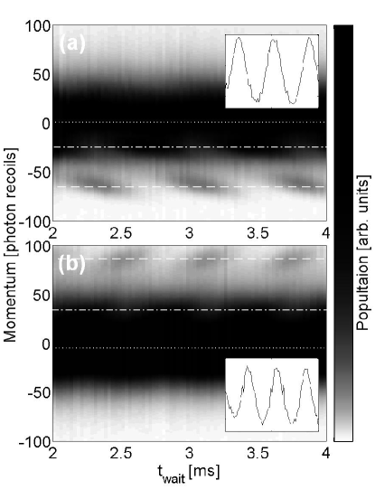
Figure 2: Experimental momentum distributions of an ensemble of cold cesium atoms after two sets of 20 pulses from an off-resonant standing light wave. There was a variable amount of time $t_{{\rm wait}}$ between the pulse sets. The dotted, dot-dashed and dashed lines denote atoms accelerated by zero, one and two sets of pulses respectively. The pulse spacing was $T=60$ $\mu$s in (a) and $T=74$ $\mu$s in (b). Each vertical slice is the momentum distribution obtained for one value of $t_{{\rm wait}}$ where the degree of shading indicates the population. Gravity is in the negative direction. The insets plot the data along the dashed lines (atoms accelerated by both pulses).

Although we have accounted for the accelerator mode revivals, we have said nothing about their sloping orientation (as seen in Fig. 2), nor about this slope’s dependence on pulse interval. An explanation for this effect can be found by returning to the earlier observation that the momentum intervals between the peaks of Fig. 1(a) change as one moves away from the center of the accelerator mode. This implies that not all parts of the distribution have to be translated by the same amount to regain the accelerator mode condition of Eq. (1). At 60 $\mu$s, the outer peaks bulge towards the center of the distribution. Assuming that the whole distribution is accelerating under gravity, the first part to regain the accelerator mode condition will be the component with the greatest positive momentum. For 74 $\mu$s the opposite will be the case and the direction of the revival’s slope will flip.

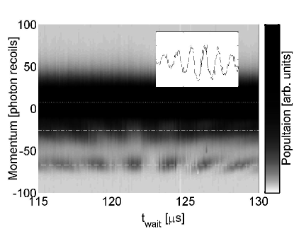
Figure 3: Experimental momentum distributions of an ensemble of cold cesium atoms after two sets of 20 pulses from an off-resonant standing light wave. Within each set the pulses were separated by $T=60$ $\mu$s and there was a variable amount of time $t_{{\rm wait}}$ between the sets. The dotted, dot-dashed and dashed lines denote atoms accelerated by zero, one and two sets of pulses respectively. Each vertical slice is the momentum distribution obtained for one value of $t_{{\rm wait}}$ where the degree of shading indicates the population. The inset plots the data along the dashed line (atoms accelerated by both pulses).

When $t_{\rm wait}$ is scanned in much smaller time steps the previous experiment can also be used to demonstrate localization in position. These experiments are only meaningful if they are performed when the wavefunction has some degree of spatial localization, that is when $t_{\rm wait}$ is close or equal to an integer multiple of the pulse separation time. Furthermore, for these wait times all the elements of the momentum comb described by Eq. (1) translate by an integer number of standing wave periods (or equivalently acquire a phase of $2\pi\times\mathop{\rm integer}$). As we have seen, the momentum distribution produced by the accelerator mode is not a comb of delta functions. Thus we do not expect an exact rephasing of the distribution even at the special wait times. Experimentally we have found that for wait times greater than three pulse separation times very little rephasing is observed. Figure 3 shows the momentum distributions observed when the pulse separation time is 60 $\mu$s and the wait time is scanned near to 120 $\mu$s. The accelerator mode reappears at the dashed line whenever the atoms prepared by the first set of pulses have moved a whole number of standing-wave wavelengths. We can quantify what the period of the reappearance or revival should be by determining the distance which the atoms move during $t_{{\rm wait}}$. This distance is given by $\Delta x=v_{0}t_{{\rm wait}}+{\frac{1}{2}}at_{{\rm wait}}^{2}$, where $v_{0}$ is the velocity of the atoms after the end of the first set of pulses. We have calculated this velocity to be 177 mm/s revival period , giving a revival period of 2.53 $\mu$s. This is in good agreement with the value of $2.56\pm 0.03$ $\mu$s that is observed along the dashed line in Fig. 3. Another important feature of this figure is that except for the exact multiple of the pulse separation time, not all parts of the accelerator mode produced by the first set of pulses are able to simultaneously undergo acceleration by the second set of pulses. This can be explained by noting that the distance moved by an atom during the wait time depends upon its initial velocity. Thus the revival period for atoms that have been accelerated the most is the smallest. This picture also provides an alternative way of understanding why we only see clear signatures of spatial localization near the multiples of $T$; the revivals from the different comb elements in the accelerator mode all come into phase at these times.

The preceding results demonstrate that by using a pulsed periodic potential it is possible to select restricted regions of phase space. We now suggest a technique for investigating the dynamical properties of these regions under the action of a chaotic potential. Our proposal is to take two atomic states which have been prepared by an accelerator mode to have identical external components. We would expose each state to chaotic potentials which differ slightly in strength and then measure the overlap between the states in order to determine the dynamics. The $F=3$ and $F=4$ ground state hyperfine levels of cesium offer a convenient means of realizing such a procedure through a technique analogous to that of a Ramsey separated field experiment Ramsey . After selecting the desired region of phase space and preparing atoms in the $F=4$, $m_{{\rm F}}=0$ state, a 50:50 superposition of the two hyperfine levels can be created by employing a $\frac{\pi}{2}$ pulse of microwave radiation resonant with the 9.19 GHz $F=3$, $m_{{\rm F}}=0\longrightarrow F=4$, $m_{{\rm F}}=0$ magnetic dipole transition. The QDKR light pulses can then be applied using the same laser beam and pulse envelope as the accelerator mode, but with the key change of moving the standing wave to make $a=0$ ResonancePRL . Importantly, each of the states in the superposition would experience the standing wave potential with a different strength. For example, light detuned 30 GHz below resonance for atoms in the $F=4$ level is detuned approximately 40 GHz for $F=3$ atoms. Since the light shift scales inversely with detuning, the component of the superposition in the $F=3$ state sees a kicking potential which is $\sim 0.75$ the size experienced by the component in $F=4$. The final step of our proposal would be to expose the superposition to a second $\frac{\pi}{2}$ microwave pulse which differs in phase by an amount $\Delta\phi$ from the first pulse. If the overlap between the two final states is good then a sinusoidal variation in the population of either state would be observed as $\Delta\phi$ were systematically changed. The exact value of the overlap could be determined by measuring the population at $\Delta\phi=0$ and $\Delta\phi=\frac{\pi}{2}$ and then using a method similar to that outlined in Ref. Gardiner97 .

To summarize, we have demonstrated a new method of preparing atoms in a narrow region of phase space from an initially broad distribution. This was achieved using quantum accelerator modes, a process in which atoms are exposed to pulses of an off-resonant standing light wave which is accelerating relative to the atoms’ frame of reference. Since the experimental configuration is very similar to that used for experiments which have studied the QDKR, it should be relatively straightforward to apply this technique to studies of quantum chaos. Previous experiments have concentrated on the ensemble behavior of the atoms. The work presented here paves the way for a more detailed examination of the dynamics. We have also suggested an experiment which would allow the production of a quantum phase space stability map. By using a method based on Ramsey separated fields we can find the amount of overlap between identical initial states which have interacted with chaotic potentials of slightly different strengths. We hope that the combination of these two ideas will eventually lead to a fuller understanding of the concepts of quantum chaos.

- (1) A.L. Lichtenberg and M.A. Lieberman, Regular and Chaotic Dynamics (Springer-Verlag, Berlin, 1992).
- (2) G. Casati et al., in Stochastic Behavior in Classical and Quantum Hamiltonian Systems, (Springer-Verlag, New York, 1979).
- (3) F.L. Moore et al., Phys. Rev. Lett. 75, 4598 (1995).
- (4) M.B. d’Arcy et al., Phys. Rev. Lett. 87, 074102 (2001).
- (5) D.A. Steck, W.H. Oskay, and M.G. Raizen, Science 293, 274 (2001).
- (6) H. Ammann et al., Phys. Rev. Lett. 80, 4111 (1998).
- (7) J. Ringot et al., Phys. Rev. Lett. 85, 2741 (2000).
- (8) A. Peres, Quantum Theory: Concepts and Methods (Kluwer Academic Publishers, Dordrecht, 1993).
- (9) M. Feingold and A. Peres, Phys. Rev. A 34, 591 (1986).
- (10) S.A. Gardiner, J.I Cirac, and P. Zoller, Phys. Rev. Lett. 79, 4790 (1997).
- (11) M.K. Oberthaler et al., Phys. Rev. Lett. 83, 4447 (1999).
- (12) S. Fishman, I. Guarneri, and L. Rebuzzini, Phys. Rev. Lett. 89, 084101 (2002).
- (13) The central diffraction order of the accelerator mode will occur at the nearest integer to .
- (14) R.M. Godun et al., Phys. Rev. A 62, 013411 (2000).
- (15) This velocity is acquired from a free fall under gravity for 5.2 ms before the beginning of the first set of accelerator mode pulses, the velocity imparted by the accelerator mode, and the free fall during the accelerator mode.
- (16) Molecular Beams, edited by N.F. Ramsey (Oxford University Press, Oxford, 1986).