Search for Long-lived States in Antiprotonic Lithium

Abstract

The spectrum of the ($Li^{3+}+\bar{p}+2e$) four-body system was calculated in an adiabatic approach. The two-electron energies were approximated by a sum of two single-electron effective charge two-center energies as suggested in Briggs . While the structure of the spectrum does not exclude the existence of long-lived states, their experimental observability is still to be clarified.

I Introduction

One of the most impressive success-stories of the last decade in few-body physics are the high-precision experimental and theoretical studies of long-lived states in antiprotonic helium exp ; kor ; elan ; kam . In view of this fact it is natural to pose the question, whether such long-lived antiprotonic states can exist in other systems, too. There were some experimental attempts to observe delayed components in annihilation products after stopping of slow antiprotons in different media wid , however, except for helium, no evidence of long-lived states was found. Theoretical predictions concerning the possible existence of such states could largely increase the willingness of experimentalists to go on with their attempts.

There are two possible directions in which further candidates for long-lived antiprotonic states could be searched for. First, one could consider atoms with electron structure similar to helium, that is, noble gases with closed outermost electron shells. This possibility was examined in some detail in Briggs with an essentially negative answer concerning the possibility of formation of long-lived states after antiproton capture in noble gases.

The second possibility is to consider the next simplest atom, the lithium, which has three electrons, one of which could be replaced by the antiproton. In order to get an idea of the possibility of the occurrence of long-lived states in this four-body system, we have performed a semi-quantitative calculation of its level structure.

II Calculation Method

The Hamiltonian of the $(Li^{3+}+\bar{p}+2e)$ four-body system can be written as

$$\hat{H}=-{1\over{2M}}\Delta_{{\bf R}}-{3\over R}+\hat{h}^{(2)}({\bf r}_{1},{\bf r}_{2};{\bf R}),$$ (1)

with the two-electron Hamiltonian

$$\hat{h}^{(2)}({\bf r}_{1},{\bf r}_{2};{\bf R})=\hat{h}^{(1)}({\bf r}_{1};{\bf R})+\hat{h}^{(1)}({\bf r}_{2};{\bf R})+{1\over|{\bf r}_{1}-{\bf r}_{2}|}$$ (2)

The single-electron two-center Hamiltonian $\hat{h}^{(1)}$ corresponds to the electron motion in the field of $Li^{3+}$ and $\bar{p}$ fixed at a distance ${\bf R}$:

$$\hat{h}^{(1)}({\bf r}_{n};{\bf R})=-{1\over{2}}\Delta_{{\bf r}_{i}}-{3\over|{\bf r}_{i}-\alpha{\bf R}|}+{1\over|{\bf r}_{i}+(1-\alpha){\bf R}|}$$ (3)

In eqs.(1-3) R  is the vector pointing from $Li^{3+}$ to $\bar{p}$, while the ${\bf r}_{i}$ are the electron coordinates measured from the $Li^{3+}-\bar{p}$ center of mass. $M$ is the reduced mass of $Li^{3+}$ and $\bar{p}$:

$${1\over M}={1\over m_{Li^{3+}}}+{1\over m_{\bar{p}}},$$

while $\alpha$ is defined as

$$\alpha={m_{\bar{p}}\over m_{Li^{3+}}+m_{\bar{p}}}\ \$$

To calculate the spectrum of this four-body system or, at least, a part of it, we have used a Born-Oppenheimer-like (BO) approximation, in which the solution of the Schrödinger-equation

$$(\hat{H}-E^{J}_{n})\Psi^{J}_{n}({\bf r}_{1},{\bf r}_{2},{\bf R})=0$$ (4)

is attempted in two successive steps. First, the equation

$$(\hat{h}^{(2)}({\bf r}_{1},{\bf r}_{2};{\bf R})-\varepsilon_{n\mu}^{(2)}(R))\Phi_{n\mu}({\bf r}_{1},{\bf r}_{2};{\bf R})=0,$$ (5)

describing the motion of two electrons in the field of $Li^{3+}$ and $\bar{p}$ separated by a fixed vector R, has to be solved. The solutions $\Phi_{n\mu}$ are characterized by the conserved quantum number $\mu$ – the sum of the electron angular momentum projections on the R  direction. Next, the total wave function $\Psi^{J}_{n}({\bf r}_{1},{\bf r}_{2},{\bf R})$ is approximated as a single product:

$$\Psi^{J}_{n}({\bf r}_{1},{\bf r}_{2},{\bf R})={u^{J}_{n\mu}(R)\over R}D^{J}_{-M_{J},-\mu}(\phi,\Theta,0)\Phi_{n\mu}({\bf r}_{1},{\bf r}_{2};{\bf R}),$$ (6)

where the Wigner’s $D$-functions are needed to ensure correct angular momentum quantum numbers $JM_{J}$ for the total wave function. The energy eigenvalues $E^{J}_{n\mu}$ are calculated from the radial equation

$$\left(-{1\over 2M}{d^{2}\over dR^{2}}+{J(J+1)-2\mu^{2}\over 2MR^{2}}-{3\over R}+\varepsilon_{n\mu}^{(2)}(R)-E^{J}_{n\mu}\right)u^{J}_{n\mu}(R)=0,$$ (7)

which is obtained by substituting Eq.(6) into Eq.(4), multiplying by $D^{J}_{-M_{J},-\mu}(\phi,\Theta,0)^{*}\Phi_{n\mu}({\bf r}_{1},{\bf r}_{2};{\bf R})^{*}$ and integrating over the electron coordinates and the angular variables $(\phi,\Theta)$ of R. In deriving Eq.(7), according to the adiabatic approximation, terms containing the derivatives of $\Phi_{n\mu}({\bf r}_{1},{\bf r}_{2};{\bf R})$ with respect to R  are neglected. In BO type calculations usually the lowermost electron configurations are used, for which $\mu=0$ (so called $\sigma$-term) in which case the $D$-function in Eq.(6) reduces to a spherical harmonics $Y_{JM_{J}}$.

For a one-electron problem Eq.(5) is replaced by

$$(\hat{h}^{(1)}({\bf r}_{i};{\bf R})-\varepsilon_{n\mu}^{(1)}(R))\varphi_{n\mu}({\bf r}_{i};{\bf R})=0$$ (8)

and it can be solved exactly by separation of variables in spheroidal coordinates $\varphi_{n\mu}({\bf r}_{i};{\bf R})$ being the well-known two-center wave functions. In our case, however, the problem of two interacting electrons in the field of two fixed Coulomb-centers is not solvable exactly and the determination of eigenvalues and eigenfunctions necessitates a highly non-trivial calculation. One could think of a variational approach of the type ahlr ; another possibility could be the diagonalization of the electron-electron interaction on the basis of two-center functions. In both cases the calculations are quite cumbersome and slowly converging when the size of the basis is increased. Since we believe, that the question of possible existence of metastability in antiprotonic lithium can be studied by a semi-qualitative exploration of its spectrum, we have chosen a simpler, elegant and efficient method of calculation for $\varepsilon_{n\mu}^{(2)}(R)$ proposed in Briggs .

The main idea of the method is to represent the two-electron energy eigenvalue as a sum of two single-electron energies:

$$\varepsilon^{(2)}(R)=\varepsilon^{(1)}_{Z_{1},Z_{2}}(R)+\varepsilon^{(1)}_{z_{1},z_{2}}(R),$$ (9)

where $\varepsilon^{(1)}_{Z_{1},Z_{2}}(R)$ and $\varepsilon^{(1)}_{z_{1},z_{2}}(R)$ are energy eigenvalues of two-center equations of the type (8) with effective charges $(Z_{1},Z_{2})$ and $(z_{1},z_{2})$ instead of the physical charges $(3,-1)$. The effective charges $(z_{1},z_{2})$ are chosen in such a way, that $\varepsilon^{(1)}_{z_{1},z_{2}}(R=0)$ and $\varepsilon^{(1)}_{z_{1},z_{2}}(R=\infty)$ should reproduce the experimental values of the first ionization potentials of $He$ atom and $Li^{+}$ ion, respectively. Thus we get $z_{1}=2.3578$ and $z_{2}=-1.0135$. As for $(Z_{1},Z_{2})$, the corresponding two-center eigenvalues in the $R=0$ and $R=\infty$ limits should reproduce the second ionization potentials of $He$ and $Li^{+}$, and the second electron is in this case the last one, therefore the physical values $Z_{1}=3$ and $Z_{2}=-1$ were taken. The electron-electron repulsion is taken into account in this method by the deviation of the effective charges $(z_{1},z_{2})$ from their physical (integer) values. In this way the approximate $\varepsilon^{(2)}(R)$ of Eq.(9) reproduces the experimental two-electron binding for the two limiting cases $R=0$ and $R=\infty$, while for intermediate $R$-values the solution of the corresponding (effective) two-center problems seems to provide a reasonable interpolation prescription. This approach has been checked in the case of $(He^{2+}+\bar{p}+2e)$ and $(Li^{3+}+\bar{p}+2e)$ systems; its results were compared with those of a detailed variational calculation of ahlr . Results of the calculations are presented in Fig.(1). The agreement of $\varepsilon^{(2)}(R)$ obtained from Eq. (9) with the variational values is amazingly good in a wide range of $R$. The same procedure was applied to calculate the energy of the first excited electron configuration, where the limiting cases were adjusted to reproduce the energies of the first excited $(1s2s)$ states of $He$ and $Li^{+}$.

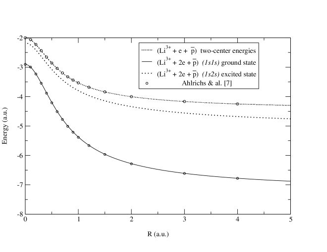
Figure 1: Electronic energies of the ($Li^{3+}+\bar{p}+2e$) and ($Li^{3+}+\bar{p}+e$) systems

Having obtained the electronic energies $\varepsilon^{(2)}(R)$ the effective potentials of Eq.(7)

$$v^{Jn}_{\text{eff}}(R)={J(J+1)\over 2MR^{2}}-{3\over R}+\varepsilon^{(2)}_{n}(R),$$ (10)

can be calculated. Here the index $\mu=0$ was omitted, while the electron configuration label $n$ can take the values $n=(1s1s),(1s2s)$. For some values of the total angular momentum $J$ the effective potentials are shown in Fig.(2) for the ground- and first excited electron configuration.

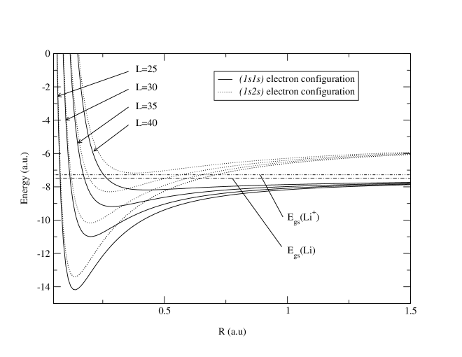
Figure 2: Effective potentials in the ($Li^{3+}+\bar{p}+2e$) system

The energy eigenvalues $E^{J\nu}_{n}$ are then calculated by solving Eq.(7) with these effective potentials, and the ”vibrational” quantum number $\nu$ is introduced to distinguish among the states with the same $J$-value.

III Results and Discussion

The resulting spectrum of the $(Li^{3+}+\bar{p}+2e)$ system is shown in Fig.(3). Apart from the energy levels of the initial system (full black circles) we have shown also the energies of daughter states which can be formed after Auger-emission of one or two electrons. The open circles correspond to the energies of the $(Li^{3+}+\bar{p}+e)$ three-particle system, while the open squares are the hydrogen-like two-particle energies of the $(Li^{3+}+\bar{p})$ system.

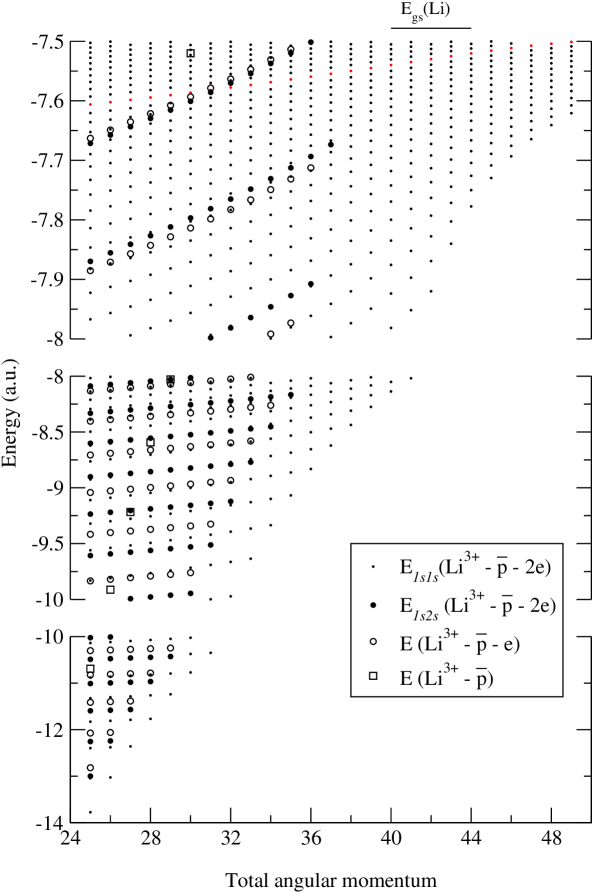
Figure 3: Spectra of antiprotonic lithium atoms

Comparing the spectra of Fig.(3) with the well-known spectra of the $He$ atomcules (see e.g. shim ), we can find some apparent similarities and differences. The basic similarity can be formulated as follows: there are many states in the spectrum, from which Auger-emission is possible only with large electron orbital momentum and therefore is strongly suppressed. This could be one reason for metastability of these states; of course, this is only a necessary condition and by no means a sufficient one.

The basic difference, on the other hand, is the much higher density of states in the expected capture region (around the $Li$ atom ground state energy) which is due to the essential difference in the electron structure of $He$ and $Li$: the last electron is strongly bound in $He$, while very loosely in $Li$.

It can be noted, that the spectrum of the $(Li^{3+}+\bar{p}+e)$ system (open circles) strongly resembles the $He$ atomcule spectrum, therefore long-lived states in an isolated $(Li^{3+}+\bar{p}+e)$ system could be certainly expected. However, in contrast to the $He$ case, this system is charged and thus its interaction with atoms of the surrounding medium might be more violent, leading to a faster collisional de-excitation of these states.

IV Conclusions

We have calculated the spectra of ($Li^{3+}+\bar{p}+2e$) and ($Li^{3+}+\bar{p}+e$) four- and three-body systems. Although the structure of the obtained spectra allows the existence of long-lived states, our calculations do not put us in a position to make definite statements about their experimental observability. This latter depends on several further factors, as well. One is the formation mechanism: for the time being we have no information about the population rate of the huge amount of states in the vicinity of expected antiproton capture energy. The physics of formation of the $(Li^{3+}+\bar{p}+2e)$ system in the reaction

$$(Li^{3+}+3e)\ +\bar{p}\ \longrightarrow(Li^{3+}+\bar{p}+2e)\ +\ e$$

is quite different from the analogous process in $He$ due to the large difference in the binding energies of the outermost electron. In the $Li$ atom the first ionization potential is only $0.198\ a.u.$, which means that even adiabatic ionization is possible: when the distance between the antiproton and $Li$ atom becomes less than $5\ a.u.$, the binding energy of the last electron in their common field becomes zero and the electron is ”pushed” into a continuum state.

Another unknown factor is the way, how the eventually formed $(Li^{3+}+\bar{p}+2e)$ systems interact with the media atoms and what is the role of collisional de-excitation in their life-time. In any case, in order to reduce the undesired effect of this factor, probably, the experiments looking for long-lived states should be performed in dilute vapors of $Li$.