Relativistic many-body calculations of transition rates from core-excited states in sodiumlike ions

Abstract

Rates and line strengths are calculated for the $2s^{2}2p^{5}3l3l^{\prime}$ - $2s^{2}2p^{6}3l^{\prime\prime}$ and $2s2p^{6}3l3l^{\prime}$ - $2s^{2}2p^{6}3l^{\prime\prime}$ electric-dipole (E1) transitions in Na-like ions with nuclear charges ranging from $Z$ = 14 to 100. Relativistic many-body perturbation theory (RMBPT), including the Breit interaction, is used to evaluate retarded E1 matrix elements in length and velocity forms. The calculations start from a $1s^{2}2s^{2}2p^{6}$ Dirac-Fock potential. First-order RMBPT is used to obtain intermediate coupling coefficients and second-order RMBPT is used to calculate transition matrix elements. A detailed discussion of the various contributions to dipole matrix elements is given for sodiumlike copper ($Z$ = 29). Transition energies used in the calculation of transition rates are from second-order RMBPT. Trends of transition rates as functions of $Z$ are shown graphically for selected transitions.

I Introduction

Transitions from $2s^{2}2p^{5}3l3l^{\prime}$ and $2s2p^{6}3l3l^{\prime}$ states to the ground ($2s^{2}2p^{6}3s$) or singly-excited ($2s^{2}2p^{6}3p$ and $2s^{2}2p^{6}3d$) states form satellite lines to the bright electric-dipole (E1) lines created by transitions from $2s^{2}2p^{5}3l$ and $2s2p^{6}3l$ states to the ground state ($2s^{2}2p^{6}$) in Ne-like ions. These core-excited $2s^{2}2p^{5}3l3l^{\prime}$ and $2s2p^{6}3l3l^{\prime}$ states (often called doubly-excited states) in sodiumlike ions have been studied extensively both experimentally and theoretically over the past 20-30 years.

Transition rates and oscillator strengths for Na-like ions have been calculated using multi-configuration Dirac-Fock (MCDF) Chen (1989); Nilsen (1989) and multi-configuration Hartree-Fock (MCHF) Zhang et al. (1989); Bruch et al. (1998a, b) methods. Recently, R-matrix calculations of electron-impact collision strengths for excitations from the inner $L$-shell into doubly excited states of Fe¹⁵⁺ was presented by Bautista (2000). Energies of $2s^{2}2p^{6}3l$ and $2s^{2}2p^{5}3l3l^{\prime}$ states were calculated in that paper using the SUPERSTRUCTURE code Eissner et al. (1974). It was shown in Bautista (2000) that disagreement between calculated data and data recommended by Sugar and Corliss (1985) and Shirai et al. (1990) ranges from 0.5% to 5%.

Experimentally, the core-excited $2s^{2}2p^{5}3l3l^{\prime}$ and $2s2p^{6}3l3l^{\prime}$ states were studied by the beam-foil technique Buchet et al. (1987); Jupén et al. (1988), photo-emission Burkhalter et al. (1979); Khakhalin et al. (1994); Akulinichev et al. (1994, 1995); Bollanti et al. (1995); Mingaleev et al. (1993); Beiersdorfer et al. (1986, 1995); Brown et al. (2001); Phillips et al. (1997), and Auger spectroscopy Schneider et al. (1989); Focke et al. (1989); Hutton et al. (1991); Schneider et al. (1995); Bliman et al. (1996). Strong line radiation involving $n$ = 3 to $n$ = 2 transitions in Ne-like ions together with satellite lines of Na-like ions were observed from laser-produced plasmas Burkhalter et al. (1979); Khakhalin et al. (1994); Akulinichev et al. (1994, 1995); Bollanti et al. (1995), X-pinch, Mingaleev et al. (1993), tokamaks Beiersdorfer et al. (1986, 1995), EBIT Brown et al. (2001), and solar flares Phillips et al. (1997). The identification of measured spectral lines was based on theoretical calculations carried out primarily using the MCDF method with Cowan’s code Cowan (1981).

In this paper, we present a comprehensive set of calculations for $2s^{2}2p^{5}3l3l^{\prime}$ - $2s^{2}2p^{6}3l^{\prime\prime}$ and $2s2p^{6}3l3l^{\prime}$ - $2s^{2}2p^{6}3l^{\prime\prime}$ transitions to compare with previous calculations and experiments. Our aim is to provide benchmark values for the entire Na isoelectronic sequence. The large number of possible transitions have made experimental identification difficult. Experimental verifications should become simpler and more reliable using this more accurate set of calculations.

Relativistic many-body perturbation theory (RMBPT) is used here to determine matrix elements and transition rates for allowed and forbidden electric-dipole transitions between the odd-parity core-excited states ($2s^{2}2p^{5}3s^{2}$ + $2s^{2}2p^{5}3p^{2}$ + $2s^{2}2p^{5}3d^{2}$ + $2s^{2}2p^{5}3s3d$ + $2s2p^{6}3s3p$ + $2s2p^{6}3p3d$) and the ground state ($2s^{2}2p^{6}3s$) together with the two singly-excited states ($2s^{2}2p^{6}3d$) and the even-parity core-excited states ($2s^{2}2p^{5}3s3p$ + $2s^{2}2p^{5}3p3d$ + $2s2p^{6}3s^{2}$ + $2s2p^{6}3p^{2}$ + $2s2p^{6}3d^{2}$ + $2s2p^{6}3s3d$) and the two singly-excited states ($2s^{2}2p^{6}3p$) in Na-like ions with nuclear charges ranging from $Z$ = 14 to 100. Retarded E1 matrix elements are evaluated in both length and velocity forms. These calculations start from a Ne-like core Dirac-Fock (DF) potential. First-order perturbation theory is used to obtain intermediate coupling coefficients and second-order RMBPT is used to determine transition matrix elements. The energies used in the calculation of transition rates are obtained from second-order RMBPT.

II Method

In this section, we discuss relativistic RMBPT for first- and second-order transition matrix elements for atomic systems with two valence electrons and one hole. Details of the RMBPT method for calculation of radiative transition rates for systems with one valence electron and one hole were presented for Ne-like and Ni-like ions in Safronova et al. (2000, 2001). Here, we follow the pattern of the corresponding calculation in Refs. Safronova et al. (2000, 2001) but limit our discussion to the model space and the first- and second-order particle-particle-hole diagram contributions in Na-like ions.

II.1 Model space

For Na-like ions with two electrons above the Ne-like ($1s^{2}2s^{2}2p_{1/2}^{2}2p_{3/2}^{4}$) core and one hole in the core, the model space is formed from particle-particle-hole states of the type $a_{v}^{\dagger}a_{w}^{\dagger}a_{a}|0\rangle$, where $|0\rangle$ is the core state function. Indices $v$ and $w$ designate valence electrons and $a$ designates a core electron. For our study of low-lying $3l3l^{\prime}2l^{-1}$ states of Na-like ions, the index $a$ ranges over $2s$, $2p_{1/2}$, and $2p_{3/2}$, while $v$ and $w$ range over $3s$, $3p_{1/2}$, $3p_{3/2}$, $3d_{3/2}$, and $3d_{5/2}$. To obtain orthonormal model states, we consider the coupled states $(vwa)$ defined by

$$\Psi(QJM)=N(Q)\sum\langle vw|K_{12}\rangle\langle K_{12}a|K\rangle a_{v}^{\dagger}a_{w}^{\dagger}a_{a}|0\rangle\,,$$ (1)

where $Q$ describes a particle-particle-hole state with quantum numbers $n_{v}\kappa_{v}n_{w}\kappa_{w}[J_{12}]n_{a}\kappa_{a}$ and intermediate momentum $J_{12}$. We use the notation $K_{i}=\{J_{i},M_{i}\}$ and $v=\{j_{v},m_{v}\}$. The sum in Eq.(1) is over magnetic quantum numbers $m_{v}$, $m_{w}$, $m_{a}$, and $M_{12}$. The quantity $\langle K_{1}K_{2}|K_{3}\rangle$ is a Clebsch-Gordan coefficient:

$$\langle K_{1}K_{2}|K_{3}\rangle=(-1)^{J_{1}-J_{2}+M_{3}}\sqrt{[J_{3}]}\left(\begin{array}[]{ccc}J_{1}&J_{2}&J_{3}\\ M_{1}&M_{2}&-M_{3}\end{array}\right)\,,$$ (2)

where $[J]=2J+1$. Combining two $n=3$ particles with possible intermediate momenta and $n=2$ hole orbitals in sodium, we obtain 121 odd-parity states with $J=1/2\,\cdots\,11/2$ and 116 even-parity states with $J=1/2\,\cdots\,11/2$. The distribution of the 237 states in the model space is found in Table I of the accompanying EPAPS document EPA . Instead of using the $3l^{\prime}3l^{\prime\prime}[J_{1}]2l^{-1}(J)$ designations, we use simpler designations $3l^{\prime}3l^{\prime\prime}[J_{1}]2l(J)$ in the tables and text below.

II.2 Dipole matrix element

The first- and second-order reduced E1 matrix elements $Z^{(1)}$, and $Z^{(2)}$, and the second-order Breit correction to the reduced E1 matrix element $B^{(2)}$ for a transition between the uncoupled particle-particle-hole state $\Psi(QJM)$ of Eq. (1) and the one-particle state $a_{x}^{\dagger}|0\rangle$ are given in Appendix.

The uncoupled reduced matrix elements are calculated in both length and velocity gauges. Differences between length and velocity forms are illustrated for the uncoupled [$3s3d_{5/2}[2]2p_{3/2}\ (1/2)$ - $3s$] matrix element in panels (a) and (b) of Fig. 1. In the high-$Z$ limit, $Z^{(1)}$ is proportional to $1/Z$, $Z^{(2)}$ is proportional to $1/Z^{2}$, and $B^{(2)}$ is independent of $Z$ (see Safronova et al. (1999)). Taking into account this $Z$-dependence, we plot $Z^{(1)}\times Z$, $Z^{(2)}\times Z^{2}$, and $B^{(2)}\times 10^{4}$ in the figure. The contribution of the second-order matrix elements $Z^{(2)}$ is seen to be much larger in length form. Differences between results in length and velocity forms shown in Fig. 1 are precisely compensated by “derivative terms” $P^{({\rm derv})}$, as shown later.

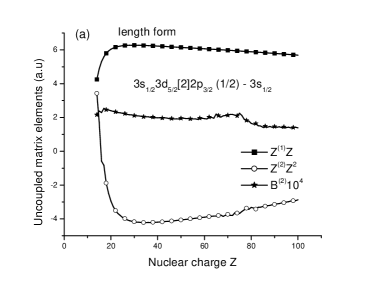
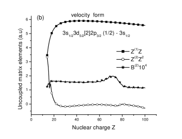
Figure 1: Uncoupled matrix element for $3s3d_{5/2}[2]2p_{3/2}\ (1/2)$–$3s$ transition calculated in length and velocity forms in Na-like ions.

Table 1: Uncoupled reduced matrix elements in length $L$ and velocity $V$ forms for transitions between the selected odd-parity core-excited states with $J$ = 1/2 and the ground $3s$ and singly-excited $3d_{3/2}$ states in Cu¹⁸⁺ ion.

$3lj3l^{\prime}j^{\prime}(J_{1})2l^{\prime\prime}j^{\prime\prime}$	$Z^{(1)}_{L}$	$Z^{(1)}_{V}$	$Z^{(2)}_{L}$	$Z^{(2)}_{V}$	$B^{(2)}_{L}$	$B^{(2)}_{V}$	$P^{(\rm derv)}_{L}$	$P^{(\rm derv)}_{V}$
[$3lj3l^{\prime}j^{\prime}[J_{1}]2l^{\prime\prime}j^{\prime\prime}\ (1/2)$– $3s_{1/2}$] transitions
$3s_{1/2}3s_{1/2}[0]2p_{1/2}$	-0.040775	-0.037586	-0.003606	-0.002838	-0.000116	-0.000104	-0.040564	0.000139
$3s_{1/2}3d_{3/2}[1]2p_{3/2}$	-0.057161	-0.052902	0.001364	0.000191	-0.000070	-0.000108	-0.057130	-0.000115
$3p_{1/2}3p_{3/2}[1]2p_{3/2}$	0.000000	0.000000	-0.000160	-0.000141	-0.000002	-0.000003	0.000000	0.000000
$3p_{1/2}3p_{3/2}[2]2p_{3/2}$	0.000000	0.000000	-0.001048	-0.001313	0.000002	0.000003	0.000000	0.000000
$3p_{3/2}3p_{3/2}[2]2p_{3/2}$	0.000000	0.000000	-0.000889	-0.001067	-0.000002	-0.000001	0.000000	0.000000
[$3lj3l^{\prime}j^{\prime}[J_{1}]2l^{\prime\prime}j^{\prime\prime}\ (1/2)$– $3d_{3/2}$] transitions
$3s_{1/2}3s_{1/2}[0]2p_{1/2}$	0.000000	0.000000	0.000388	-0.000293	0.000006	0.000003	0.000000	0.000000
$3s_{1/2}3d_{3/2}[1]2p_{3/2}$	0.012526	0.011536	0.001077	0.000835	0.000027	0.000013	0.012483	-0.000003
$3p_{1/2}3p_{3/2}[1]2p_{3/2}$	0.000000	0.000000	0.000205	0.000602	-0.000001	-0.000001	0.000000	0.000000
$3p_{1/2}3p_{3/2}[2]2p_{3/2}$	0.000000	0.000000	0.000720	-0.000132	-0.000002	0.000001	0.000000	0.000000
$3p_{3/2}3p_{3/2}[2]2p_{3/2}$	0.000000	0.000000	0.000671	0.000436	0.000004	0.000002	0.000000	0.000000

Table 2: Wavelengths ($\lambda$ in Å) and transition rates ($A_{r}$ in $s^{-1}$) for transitions from core-excited states $QJ$ ($Q=3lj3l^{\prime}j^{\prime}[J_{1}]2l^{\prime\prime}j^{\prime\prime}$, $J=1/2$ ) to the ground state in Na-like ions. Comparison with theoretical data obtained by using YODA code from Ref. Nilsen (1989). Numbers in brackets represent powers of 10.

Q	$Z$ = 26				$Z$ = 54
	$\lambda_{\rm RMBPT}$	$\lambda_{\rm YODA}$	$A_{r}^{\rm RMBPT}$	$A_{r}^{\rm YODA}$	$\lambda_{\rm RMBPT}$	$\lambda_{\rm YODA}$	$A_{r}^{\rm RMBPT}$	$A_{r}^{\rm YODA}$
$3s_{1/2}3s_{1/2}[0]2p_{1/2}$	17.0747	17.1207	8.096[11]	8.27[11]	2.7865	2.7884	2.507[12]	2.62[12]
$3s_{1/2}3d_{3/2}[1]2p_{3/2}$	15.9418	15.9883	9.449[10]	1.10[11]	2.7731	2.7747	9.345[10]	6.70[10]
$3p_{1/2}3p_{1/2}[0]2p_{1/2}$	15.6327	15.6671	2.578[09]	2.67[09]	2.7355	2.7366	2.625[14]	2.50[14]
$3s_{1/2}3d_{3/2}[2]2p_{3/2}$	15.5711	15.5958	4.600[11]	5.21[11]	2.7241	2.7251	1.724[14]	2.07[14]
$3s_{1/2}3d_{5/2}[2]2p_{3/2}$	15.5029	15.5193	3.776[12]	4.02[12]	2.6271	2.6276	4.846[11]	6.35[11]
$3p_{1/2}3p_{3/2}[1]2p_{1/2}$	15.3681	15.3884	1.465[11]	1.56[11]	2.5927	2.5939	8.932[10]	1.06[12]
$3p_{3/2}3p_{3/2}[0]2p_{1/2}$	15.3672	15.3558	9.425[08]	7.81[09]	2.5925	2.5938	9.882[11]	6.29[10]
$3s_{1/2}3d_{3/2}[1]2p_{1/2}$	15.2148	15.2174	2.240[13]	2.65[13]	2.5734	2.5748	9.387[11]	6.72[11]
$3s_{1/2}3p_{1/2}[0]2s_{1/2}$	14.0969	14.1212	2.826[10]	2.80[10]	2.5572	2.5580	5.078[13]	6.02[13]
$3d_{5/2}3d_{5/2}[0]2p_{1/2}$	13.6959	13.6884	9.156[07]	1.67[09]	2.3876	2.3881	2.952[08]	1.43[10]

II.3 Dipole matrix elements in Cu¹⁸⁺

In Table 1, we list values of uncoupled first- and second-order dipole matrix elements $Z^{(1)}$, $Z^{(2)}$, $B^{(2)}$, together with derivative terms $P^{({\rm derv})}$ for Na-like copper, $Z$ = 29. For simplicity, we only list values for selected dipole transitions between odd-parity states with $J$ = 1/2 and the ground $3s$ and excited $3d_{3/2}$ states. Uncoupled matrix elements for other transitions in Na-like copper are given in Table II of the accompanying EPAPS document EPA . The derivative terms shown in Table 1 arise because transition amplitudes depend on energy, and the transition energy changes order-by-order in RMBPT calculations. Both length ($L$) and velocity ($V$) forms are given for the matrix elements. We find that the first-order matrix elements $Z^{(1)}_{L}$ and $Z^{(1)}_{V}$ differ by 10%; the $L$ - $V$ differences between second-order matrix elements are much larger for some transitions. The term $P^{({\rm derv)}}$ in length form almost equals $Z^{(1)}$ in length form but $P^{({\rm derv)}}$ in velocity form is smaller than $Z^{(1)}$ in velocity form by three to four orders of magnitude.

Although we use an intermediate-coupling scheme, it is nevertheless convenient to label the physical states using the $LS$ scheme. Length and velocity forms of coupled matrix elements differ only in the fourth or fifth digits. These $L$ - $V$ differences arise because we start our RMBPT calculations using a non-local Dirac-Fock potential. If we were to replace the DF potential by a local potential, the differences would disappear completely. Removing the second-order contribution increases $L$ - $V$ differences by a factor of 10. Values of coupled reduced matrix elements in length and velocity forms are given in Table III of the accompanying EPAPS document EPA . Theoretical wavelengths ${\lambda}$ and transition probabilities $A_{r}$ for selected transitions in Na-like from $Z$ = 26 up to $Z$ = 30 are given in Table IV of EPA .

Table 3: Wavelengths ($\lambda$ in Å) and transition rates ($A_{r}$ in $s^{-1}$)for transitions between core-excited states $3l3l^{\prime}(L_{1}S_{1})2p\ LSJ$ and singly-excited states $3l\ L^{\prime}S^{\prime}J^{\prime}$ in Na-like ions. Comparison with experimental data ($\lambda_{\rm expt}$) from Ref. Burkhalter et al. (1979). Numbers in brackets represent powers of 10.

Upper level	Low level	$Z$ = 26
		$\lambda_{\rm RMBPT}$	$\lambda_{\rm expt}$	$A_{r}$
$3s3p(^{3}P)2p\ ^{2}S_{1/2}$	$3p\ ^{2}P_{3/2}$	16.813	16.821	9.189[10]
$3s3d(^{3}D)2p\ ^{2}P_{3/2}$	$3d\ ^{2}D_{3/2}$	16.839	18.834	2.942[11]
$3s3p(^{3}P)2p\ ^{2}D_{3/2}$	$3p\ ^{2}P_{1/2}$	16.883	16.899	9.942[10]
$3s3p(^{3}P)2p\ ^{2}P_{1/2}$	$3p\ ^{2}P_{1/2}$	16.939	16.937	2.782[10]
$3s3d(^{3}D)2p\ ^{2}P_{1/2}$	$3d\ ^{2}D_{3/2}$	16.958	16.952	4.962[11]
$3s3p(^{3}P)2p\ ^{2}P_{1/2}$	$3p\ ^{2}P_{3/2}$	16.999	16.993	7.880[11]
$3s3d(^{1}D)2p\ ^{2}P_{3/2}$	$3d\ ^{2}D_{5/2}$	17.037	17.029	5.370[11]
$3p3p(^{3}P)2p\ ^{2}P_{3/2}$	$3d\ ^{2}D_{3/2}$	17.098	17.094	3.901[11]
$3s3d(^{1}D)2p\ ^{2}D_{5/2}$	$3d\ ^{2}D_{3/2}$	17.131	17.129	4.887[11]
$3s3d(^{3}D)2p\ ^{4}F_{3/2}$	$3d\ ^{2}D_{3/2}$	17.168	17.166	4.273[11]
$3s3p(^{1}P)2p\ ^{2}P_{3/2}$	$3p\ ^{2}P_{3/2}$	17.199	17.208	5.081[11]
$3s3p(^{3}P)2p\ ^{4}P_{3/2}$	$3p\ ^{2}P_{3/2}$	17.242	17.244	1.972[11]
$3s3p(^{3}P)2p\ ^{4}D_{1/2}$	$3p\ ^{2}P_{3/2}$	17.307	17.297	1.118[11]
$3s3d(^{3}D)2p\ ^{2}P_{3/2}$	$3d\ ^{2}D_{5/2}$	17.353	17.344	7.288[11]
$3s3s(^{1}S)2p\ ^{2}P_{3/2}$	$3s\ ^{2}S_{1/2}$	17.374	17.368	7.925[11]
$3p3p(^{3}P)2p\ ^{2}D_{5/2}$	$3d\ ^{2}D_{3/2}$	17.394	17.398	3.118[11]
$3s3d(^{1}D)2p\ ^{2}P_{1/2}$	$3d\ ^{2}D_{3/2}$	17.401	17.407	6.364[11]
$3s3p(^{1}P)2p\ ^{2}S_{1/2}$	$3p\ ^{2}P_{3/2}$	17.454	17.451	7.665[11]
$3s3p(^{1}P)2p\ ^{2}P_{1/2}$	$3p\ ^{2}P_{1/2}$	17.484	17.471	5.848[11]
$3s3d(^{3}D)2p\ ^{4}F_{7/2}$	$3d\ ^{2}D_{5/2}$	17.493	17.499	1.394[11]
$3s3p(^{1}P)2p\ ^{2}P_{1/2}$	$3p\ ^{2}P_{3/2}$	17.548	17.542	1.810[10]
$3p3p(^{3}P)2p\ ^{4}D_{1/2}$	$3d\ ^{2}D_{3/2}$	17.596	17.596	6.959[10]
$3s3p(^{3}P)2p\ ^{4}S_{3/2}$	$3p\ ^{2}P_{1/2}$	17.611	17.623	2.480[09]
$3s3p(^{3}P)2p\ ^{4}S_{3/2}$	$3p\ ^{2}P_{3/2}$	17.677	17.660	1.185[10]
$3p3p(^{3}P)2p\ ^{4}D_{5/2}$	$3d\ ^{2}D_{3/2}$	17.736	17.734	1.366[10]
$3p3p(^{1}D)2p\ ^{2}D_{5/2}$	$3d\ ^{2}D_{5/2}$	17.763	17.787	1.443[10]
$3p3p(^{3}P)2p\ ^{4}P_{3/2}$	$3d\ ^{2}D_{5/2}$	17.821	17.821	2.537[10]
$3p3p(^{3}P)2p\ ^{4}P_{3/2}$	$3d\ ^{2}D_{5/2}$	17.882	17.901	1.892[10]

Table 4: Wavelengths ($\lambda$ in Å) and transition rates ($A_{r}$ in $s^{-1}$) for transitions between core-excited states $3l3l^{\prime}(L_{1}S_{1})2p\ LSJ$ and singly-excited states $3l\ L^{\prime}S^{\prime}J^{\prime}$ in Na-like ions. Comparison with experimental data ($\lambda_{\rm expt}$) from Ref. Akulinichev et al. (1994) ($a$) and Ref. Brown et al. (2001) ($b$). Numbers in brackets represent powers of 10.

Upper level	Low level	$Z$ = 26			$Z$ = 27
		$\lambda_{\rm RMBPT}$	$\lambda_{\rm expt}$	$A_{r}$	$\lambda_{\rm RMBPT}$	$\lambda_{\rm expt}$	$A_{r}$
$3p3d(^{1}S)2p\ ^{2}D_{3/2}$	$3p\ ^{2}P_{1/2}$	15.057		5.532[11]	13.667	13.667a	7.187[11]
$3p3d(^{1}S)2p\ ^{2}D_{5/2}$	$3p\ ^{2}P_{3/2}$	15.090		1.272[12]	13.704	13.707a	2.067[12]
$3d3d(^{1}S)2p\ ^{2}P_{1/2}$	$3d\ ^{2}D_{3/2}$	15.092	15.093a	5.375[12]	13.695		6.534[12]
$3s3d(^{3}D)2p\ ^{2}P_{3/2}$	$3s\ ^{2}S_{1/2}$	15.119	15.115b	8.210[12]	13.718		1.008[13]
$3p3d(^{3}D)2p\ ^{2}S_{1/2}$	$3p\ ^{2}P_{1/2}$	15.150	15.142a	8.704[10]	13.744		1.996[11]
$3p3d(^{1}S)2p\ ^{2}D_{3/2}$	$3p\ ^{2}P_{3/2}$	15.166		3.835[12]	13.775	13.773a	4.836[12]
$3d3d(^{3}P)2p\ ^{2}P_{3/2}$	$3d\ ^{2}D_{3/2}$	15.181	15.182a	9.080[12]	13.774		1.146[13]
$3s3d(^{3}D)2p\ ^{2}P_{1/2}$	$3s\ ^{2}S_{1/2}$	15.215	15.208b	2.240[13]	13.805		2.723[13]
$3p3d(^{3}P)2p\ ^{2}P_{1/2}$	$3p\ ^{2}P_{1/2}$	15.237		1.430[13]	13.823	13.823a	1.699[13]
$3s3d(^{1}D)2p\ ^{2}P_{3/2}$	$3s\ ^{2}S_{1/2}$	15.272	15.26b	1.340[13]	13.855		1.614[13]
$3s3d(^{1}D)2p\ ^{2}P_{3/2}$	$3s\ ^{2}S_{1/2}$	15.272	15.280a	1.340[13]	13.855		1.614[13]
$3p3d(^{3}P)2p\ ^{2}P_{1/2}$	$3p\ ^{2}P_{3/2}$	15.286	15.289a	1.536[11]	13.872		9.115[10]
$3d3d(^{3}F)2p\ ^{2}F_{5/2}$	$3d\ ^{2}D_{5/2}$	15.361	15.360a	1.002[12]	13.930		1.691[12]
$3d3d(^{3}F)2p\ ^{2}D_{5/2}$	$3d\ ^{2}D_{3/2}$	15.369		6.618[12]	13.943	13.940a	9.585[12]
$3p3d(^{3}D)2p\ ^{4}F_{3/2}$	$3p\ ^{2}P_{3/2}$	15.429		3.019[09]	14.014	14.015a	1.919[09]
$3s3d(^{3}D)2p\ ^{4}D_{3/2}$	$3s\ ^{2}S_{1/2}$	15.435		1.742[12]	14.004	14.000a	2.880[12]
$3p3d(^{1}D)2p\ ^{2}D_{3/2}$	$3p\ ^{2}P_{1/2}$	15.510		3.134[11]	14.079	14.078a	4.868[11]
$3s3d(^{3}D)2p\ ^{2}P_{3/2}$	$3s\ ^{2}S_{1/2}$	15.525		2.997[12]	14.091	14.093a	3.817[12]
$3d3d(^{3}F)2p\ ^{4}F_{3/2}$	$3d\ ^{2}D_{5/2}$	15.561	15.568a	1.746[11]	14.129		2.141[11]
$3d3d(^{1}D)2p\ ^{2}F_{7/2}$	$3d\ ^{2}D_{5/2}$	15.573		6.467[11]	14.143	14.148a	7.639[11]

Table 5: Wavelengths ($\lambda$ in Å) and transition rates ($A_{r}$ in $s^{-1}$) for transitions between core-excited states $3l3l^{\prime}(L_{1}S_{1})2p\ LSJ$ and singly-excited states $3l\ L^{\prime}S^{\prime}J^{\prime}$ in Na-like ions. Comparison with experimental data ($\lambda_{\rm expt}$) from Ref. Akulinichev et al. (1994). Numbers in brackets represent powers of 10.

Upper level	Low level	$Z$ = 29			$Z$ = 28			$Z$ = 30
		$\lambda_{\rm RMBPT}$	$\lambda_{\rm expt}$	$A_{r}$	$\lambda_{\rm RMBPT}$	$\lambda_{\rm expt}$	$A_{r}$	$\lambda_{\rm RMBPT}$	$\lambda_{\rm expt}$	$A_{r}$
$3s3s(^{1}S)2s\ ^{2}S_{1/2}$	$3p\ ^{2}P_{1/2}$	11.407	11.403	8.906[12]	12.466	12.461	7.918[12]	10.475	10.481	9.805[12]
$3d3d(^{1}S)2p\ ^{2}P_{1/2}$	$3d\ ^{2}D_{3/2}$	11.425	11.427	9.183[12]	12.484	12.492	7.808[12]	10.494	10.493	1.065[13]
$3d3d(^{3}P)2p\ ^{2}P_{3/2}$	$3d\ ^{2}D_{3/2}$	11.488	11.480	1.611[13]	12.554	12.556	1.383[13]	10.551		1.819[13]
$3p3d(^{3}D)2p\ ^{2}S_{1/2}$	$3p\ ^{2}P_{3/2}$	11.506	11.503	3.173[13]	12.572		2.698[13]	10.569		3.654[13]
$3d3d(^{3}F)2p\ ^{2}D_{3/2}$	$3d\ ^{2}D_{5/2}$	11.514		1.413[13]	12.581		1.236[13]	10.576	10.573	1.566[13]
$3d3d(^{1}G)2p\ ^{2}F_{7/2}$	$3d\ ^{2}D_{5/2}$	11.537	11.538	2.019[13]	12.592	12.596	1.686[13]	10.593		2.410[13]
$3p3d(^{3}P)2p\ ^{2}D_{3/2}$	$3p\ ^{2}P_{1/2}$	11.552		2.305[13]	12.624	12.623	2.555[13]	10.606		9.851[12]
$3p3d(^{3}P)2p\ ^{4}D_{3/2}$	$3p\ ^{2}P_{1/2}$	11.560	11.561	1.012[13]	12.639		3.548[12]	10.616		2.617[13]
$3d3d(^{3}F)2p\ ^{2}F_{5/2}$	$3d\ ^{2}D_{5/2}$	11.615		3.112[12]	12.694		2.364[12]	10.664	10.664	4.022[12]
$3p3d(^{3}P)2p\ ^{2}P_{3/2}$	$3p\ ^{2}P_{3/2}$	11.624	11.620	1.252[12]	12.706	12.700	9.215[11]	10.674		1.493[12]
$3d3d(^{3}F)2p\ ^{2}D_{5/2}$	$3d\ ^{2}D_{5/2}$	11.634		1.438[12]	12.714		1.553[12]	10.683	10.687	1.858[12]
$3d3d(^{3}P)2p\ ^{4}S_{3/2}$	$3d\ ^{2}D_{5/2}$	11.662		4.945[12]	12.730	12.736	3.862[12]	10.723	10.721	6.355[12]
$3p3d(^{3}D)2p\ ^{4}D_{5/2}$	$3p\ ^{2}P_{3/2}$	11.673	11.673	9.418[11]	12.744		1.890[09]	10.729		2.888[12]
$3s3d(^{3}D)2p\ ^{4}D_{3/2}$	$3s\ ^{2}S_{1/2}$	11.688	11.685	7.023[12]	12.767		4.600[12]	10.740	10.738	1.021[13]
$3d3d(^{3}P)2p\ ^{4}D_{1/2}$	$3d\ ^{2}D_{3/2}$	11.701		1.809[13]	12.775	12.772	1.361[13]	10.758		2.344[13]
$3d3d(^{3}F)2p\ ^{4}F_{5/2}$	$3d\ ^{2}D_{3/2}$	11.723		9.844[12]	12.804		6.190[12]	10.774	10.778	1.268[13]
$3s3d(^{3}D)2p\ ^{4}D_{1/2}$	$3s\ ^{2}S_{1/2}$	11.736	11.737	7.629[12]	12.822		6.064[12]	10.782		9.682[12]
$3d3d(^{1}G)2p\ ^{2}G_{7/2}$	$3d\ ^{2}D_{5/2}$	11.755	11.755	7.229[12]	12.836	12.835	5.328[12]	10.825		9.462[12]
$3p3d(^{3}D)2p\ ^{4}D_{1/2}$	$3p\ ^{2}P_{3/2}$	11.785	11.784	5.716[11]	12.864		4.781[11]	10.837		6.885[11]

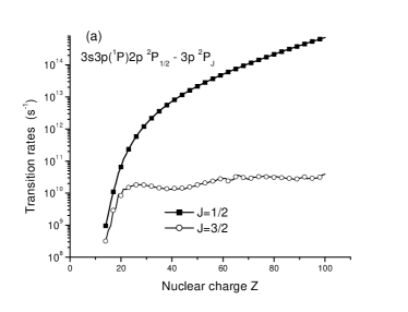
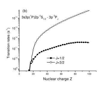
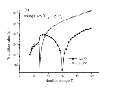
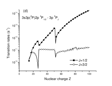
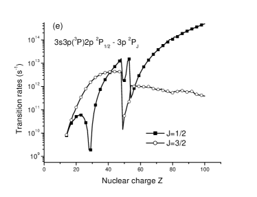
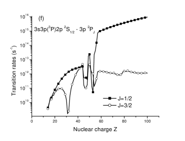
Figure 2: Transition rates for the transitions from core-excited even-parity states with $J$ = 1/2 as function of $Z$ in Na-like ions.

III Results and comparison with other theory and experiment

Trends of the $Z$-dependence of transition rates for the transitions from core-excited even-parity states with $J$ = 1/2 to two possible singly-excited odd-parity states are presented in Fig. 2. Figures for transitions from other states are found in the accompanying EPAPS document EPA .

We find that transitions with smooth $Z$-dependence are rarer than transitions with sharp features. Smooth $Z$-dependence occurs for transitions from doublet and quartet core-excited states. Usually, singularities occur in the intermediate interval of $Z$ = 25 - 50 when neither $LS$ nor $jj$ coupling schemes describe the states of these ions properly. One general conclusion that can be derived from the figures is that the smooth $Z$-dependence occurs more frequently for transitions from low-lying core-excited states.

Singularities in the transition-rate curves have two distinct origins: avoided level crossings and zeros in dipole matrix elements. Avoided level crossings result in changes of the dominant configuration of a state at a particular value of $Z$ and lead to abrupt changes in the transition rate curves when the partial rates associated with the dominant configurations below and above the crossing point are significantly different. Zeros in transition matrix elements lead to cusp-like minima in the transition rate curves. Examples of each of these two singularity types can be seen in Fig. 2.

In Table  2, we present data for transitions from odd-parity states with $J=1/2$ in Fe⁺¹⁵ and Xe⁺⁴³. We compare the present RMBPT values with those given by Nilsen (1989). More complete comparisons are given in the accompanying EPAPS document EPA . The calculations of Nilsen (1989) were based on a multiconfigurational relativistic bound-state and distorted-wave continuum code (YODA). Since $jj$ labeling was used in Nilsen (1989), we keep that labeling in Table 2. We find that the $A_{r}$-values from RMBPT and YODA differ by 10% in most cases. The differences are explained by the second-order corrections to dipole matrix elements included in RMBPT.

In Tables 3 - 5, wavelengths and electric-dipole transition rates are presented for transitions in Na-like Fe, Co, Ni, Cu and Zn. We limit the tables to transitions given in Refs. Burkhalter et al. (1979); Akulinichev et al. (1994); Brown et al. (2001). Measurements for Fe¹⁵⁺ are presented in Tables  3 and 4 since two different ranges of spectra were investigated in Ref. Burkhalter et al. (1979) (16.8 - 17.8 Å) and Ref. Akulinichev et al. (1994) (15.1 - 15.5 Å). Three lines for Fe¹⁵⁺ were identified in region (15.1 - 15.26 Å) by Brown et al. in Ref. Brown et al. (2001). All possible $3l_{1}j_{1}3l_{2}j_{2}[J_{1}]2l_{3}j_{3}(J)$ - $3l_{j}$ transitions produce 393 spectrum lines. These lines in Fe¹⁵⁺ are covered by four spectral regions; 12.5 - 14.2 Å  (114 lines), 15.1 - 15.9 Å  (174 lines), 16.8 - 17.9 Å  (102 lines), and 19.3 - 19.7 Å  (3 lines). The first 114 lines are from $3dj_{1}3dj_{2}[J_{1}]2s(J)$ - $3l_{j}$ and $3pj_{1}3dj_{2}[J_{1}]2s_{1/2}(J)$ - $3l_{j}$ transitions and the last three lines are from $3s3s[0]2p_{j}(J)$ - $3d_{j}$ transitions. Our RMBPT data together with experimental measurements for Fe¹⁵⁺ in the region of 16.8 - 17.8 Å  and 15.1 - 15.5 Å  are presented in Tables 3 and 4, respectively. The agreement between our RMBPT wavelengths and the experimental values is 0.02 - 0.04% for both regions of the spectrum.

IV Conclusion

We have presented a systematic second-order relativistic MBPT study of reduced matrix elements and transition rates for [$3l_{1}j_{1}3l_{2}j_{2}[J_{1}]2l_{3}j_{3}\ (J)$ - $3lj$] electric-dipole transitions in sodiumlike ions with the nuclear charges $Z$ ranging from 14 to 100. Our retarded $E1$ matrix elements include correlation corrections from Coulomb and Breit interactions. Both length and velocity forms of the matrix elements were evaluated and small differences (0.4% - 1%), caused by the non locality of the starting DF potential, were found between the two forms. Second-order RMBPT transition energies were used in our evaluation of transition rates. These calculations were compared with other calculations and with available experimental data. For $Z\geq 20$, we believe that the present theoretical data are more accurate than other theoretical or experimental data for transitions between the $3l_{1}j_{1}3l_{2}j_{2}[J_{1}]2l_{3}j_{3}\ (J)$ core-excited states and the $3lj$ singly-excited states in Na-like ions. We hope that these results will be useful in analyzing older experiments and planning new ones. Additionally, these calculations provide basic theoretical input amplitudes for calculations of reduced matrix elements, oscillator strengths and transition rates for Cu-like satellites to transitions in Ni-like ions.

*

Appendix A The particle-particle-hole diagram contribution for dipole matrix element

The first-order reduced E1 matrix element $Z^{(1)}$ for a transition between the uncoupled particle-particle-hole state $\Psi(QJM)$ of Eq. (1) and the one-particle state $a_{x}^{\dagger}|0\rangle$ is

$$Z^{(1)}(v^{0}w^{0}\left[J_{12}\right]aJ,xJ^{\prime})=\sum_{vw}\sqrt{[J_{12}][J]}P_{J_{12}}(v^{0}v,w^{0}w)\delta(J^{\prime}x)\delta(vx)Z(va)\left\{\begin{array}[]{lll}j_{x}&J&1\\ j_{a}&j_{w}&J_{12}\end{array}\right\}(-1)^{-j_{a}+j_{w}},$$ (3)

where $v$, $w$ range over $\{v^{0},w^{0}\}$. The quantity $P_{J}(v^{0}v,w^{0}w)$ is a symmetry coefficient defined by

$$P_{J}(v^{0}v,w^{0}w)=\eta_{v^{0}w^{0}}\left[\delta_{v^{0}v}\delta_{w^{0}w}+(-1)^{j_{v}+j_{w}+J+1}\delta_{v^{0}w}\delta_{w^{0}v}\right],$$ (4)

where $\eta_{vw}$ is a normalization factor given by

$$\eta_{vw}=\left\{\begin{array}[]{ll}1&\mbox{for $w\neq v$}\\ 1/\sqrt{2}&\mbox{for $w=v$}.\end{array}\right.$$

The dipole matrix element $Z(va)$, which includes retardation, is given in velocity and length forms in Eqs.(3,4) of Ref. Safronova et al. (1999). The second-order reduced matrix element $Z^{(2)}(v^{0}w^{0}\left[J_{12}\right]aJ,xJ^{\prime})$ consists of four contributions: $Z^{({\rm HF})}$, $Z^{({\rm RPA})}$, $Z^{({\rm corr})}$, and $Z^{({\rm derv})}$.

$$Z^{(\mathrm{HF})}(v^{0}w^{0}\left[J_{12}\right]aJ,xJ^{\prime})=\sum_{vw}\sqrt{[J_{12}][J]}P_{J_{12}}(v^{0}v,w^{0}w)\delta(J^{\prime}x)\delta(vx)(-1)^{-j_{a}+j_{w}}$$

$$\times\left\{\begin{array}[]{lll}j_{x}&J&1\\ j_{a}&j_{w}&J_{12}\end{array}\right\}\sum_{i}\left[\frac{\delta(j_{w}j_{i})\Delta(wi)Z(ia)}{\epsilon(w)-\epsilon(i)}+\frac{\Delta(ia)\delta(j_{a},j_{i})Z(wi)}{\epsilon(a)-\epsilon(i)}\right]$$ (7)

$$Z^{({\rm RPA})}(v^{0}w^{0}\left[J_{12}\right]aJ,xJ^{\prime}) = \frac{1}{3}\sum_{vw}\sqrt{[J_{12}][J]}P_{J_{12}}(v^{0}v,w^{0}w)\delta(J^{\prime}x)\delta(vx)\left\{\begin{array}[]{lll}j_{x}&J&1\\ j_{a}&j_{w}&J_{12}\end{array}\right\}(-1)^{-j_{a}+j_{w}}$$ (10)

$$\times \sum_{nb}\left[\frac{Z_{1}(wban)Z(bn)}{\epsilon(b)+\epsilon(w)-\epsilon(a)-\epsilon(n)}+\frac{Z_{1}(wnab)Z(nb)}{\epsilon(b)+\epsilon(a)-\epsilon(w)-\epsilon(n)}\right]$$ (11)

$$Z^{({\rm corr})}(v^{0}w^{0}\left[J_{12}\right]aJ,xJ^{\prime}) = \sum_{vw}\sqrt{[J_{12}][J]}P_{J_{12}}(v^{0}v,w^{0}w)\delta(J^{\prime}x)\sum_{k}(-1)^{j_{a}-j_{v}+J_{12}+k}$$ (14)

$$\times \sum_{i}\left[\frac{Z(ix)X_{k}(vwai)}{\epsilon(v)+\epsilon(w)-\epsilon(a)-\epsilon(i)}\delta(J,j_{i})\frac{1}{[J]}\left\{\begin{array}[]{lll}j_{w}&j_{i}&k\\ j_{a}&j_{v}&J_{12}\end{array}\right\}\right.$$

$$- \left.\frac{Z(ia)X_{k}(vwxi)}{\epsilon(v)+\epsilon(w)-\epsilon(x)-\epsilon(i)}\left\{\begin{array}[]{lll}j_{x}&j_{i}&J_{12}\\ j_{w}&j_{v}&k\end{array}\right\}\left\{\begin{array}[]{lll}j_{x}&J&1\\ j_{a}&j_{i}&J_{12}\end{array}\right\}(-1)^{J+j_{w}-j_{i}}\right.$$ (19)

$$- \left.\frac{Z(vi)Z_{k}(axwi)}{\epsilon(a)+\epsilon(x)-\epsilon(w)-\epsilon(i)}\left\{\begin{array}[]{lll}j_{v}&J&k\\ j_{a}&j_{w}&J_{12}\end{array}\right\}\left\{\begin{array}[]{lll}j_{x}&J&1\\ j_{v}&j_{i}&k\end{array}\right\}(-1)^{k+J_{12}+j_{w}+j_{i}-J+1}\right]$$ (24)

In the above equations, the index $b$ designates core states, index $n$ designates excited states, and index $i$ denotes an arbitrary core or excited state. In the sums over $i$ in Eqs. (A,24), all terms with vanishing denominators are excluded. The definitions of $X_{k}(abcd)$ and $Z_{k}(abcd)$ are given by Eq.(2.12) and Eq.(2.15) in Ref. Safronova et al. (1996) and $\Delta_{ij}$ is defined at the end of section II in Safronova et al. (1996); $\epsilon(w)$ is a one-electron DF energy.

The derivative term is just the derivative of the the first-order matrix element with respect to the transition energy. It is introduced to account for the first-order change in transition energy. An auxiliary quantity $P^{({\rm derv})}$ is defined by

$$P^{({\rm derv})}(v^{0}w^{0}\left[J_{12}\right]aJ,xJ^{\prime})=\sum_{vw}\sqrt{[J_{12}][J]}P_{J_{12}}(v^{0}v,w^{0}w)\delta(J^{\prime}x)\delta(vx)Z^{({\rm derv})}(va)\left\{\begin{array}[]{lll}j_{x}&J&1\\ j_{a}&j_{w}&J_{12}\end{array}\right\}(-1)^{-j_{a}+j_{w}}.$$ (25)

The derivative term $Z^{({\rm derv)}}(va)$ is given in length and velocity forms by Eqs. (10) and (11) of Ref. Safronova et al. (1999).

The coupled dipole transition matrix element between the initial state $I$ and final state $F$ in Na-like ions is given by

$$Q^{(1+2)}(I-F) = -\frac{1}{E^{(1)}[F]-E^{(1)}[I]}\sum_{avw}\sum_{J_{12}^{\prime}}C_{1}^{F}[vw[J_{12}^{\prime}]a(J)]$$ (26)

$$\times \left\{\left[\epsilon(x)-\epsilon(vwa)\right]\left[Z^{(1+2{\rm)}}[vw\left[J_{12}^{\prime}\right]aJ,xJ^{\prime}]+B^{(2)}[vw\left[J_{12}^{\prime}\right]aJ,xJ^{\prime}]\right]\right.$$

$$+ \left.\left[-E^{(1)}[F]+E^{(1)}[I]-\epsilon(x)+\epsilon(vwa)\right]P^{({\rm derv)}}[vw\left[J_{12}^{\prime}\right]aJ,xJ^{\prime}]\right\}.$$

Here, $\epsilon(vwa)=\epsilon(v)+\epsilon(w)-\epsilon(a)$, $Z^{(1+2)}=Z^{(1)}+Z^{({\rm RPA})}+Z^{({\rm corr})}$. (Note that $Z^{({\rm HF})}$ vanishes since we start from a Hartree-Fock basis.) The sum over $vwa,\,J_{12}^{\prime}$ is understood as sum over the complex of states with the same $J$ and parity. In Eq. (26), we let $B^{(2)}=B^{({\rm RPA})}+B^{({\rm HF)}}$ +$B^{({\rm corr})}$ to represent second-order corrections arising from the Breit interaction. The quantities $C_{1}^{F}[vw[J_{12}^{\prime}]a(J)]$ are eigenvectors (or mixing coefficients) for particle-particle-hole state $F$. The initial state $I$ is a single, one-valence state. Using the above formulas and the results for uncoupled reduced matrix elements, we carry out the transformation from uncoupled reduced matrix elements to intermediate coupled matrix elements between physical states.

References

- Chen (1989) M. H. Chen, Phys. Rev. A 40, 2365 (1989).
- Nilsen (1989) J. Nilsen, At. Data Nucl. Data Tables 41, 131 (1989).
- Zhang et al. (1989) H. L. Zhang, D. H. Sampson, R. E. H. Clark, and J. B. Mann, At. Data Nucl. Data Tables 41, 1 (1989).
- Bruch et al. (1998a) R. Bruch, U. I. Safronova, A. S. Shlyaptseva, J. Nilsen, and D. Schneider, Phys. Scr. 57, 334 (1998a).
- Bruch et al. (1998b) R. Bruch, U. I. Safronova, A. S. Shlyaptseva, J. Nilsen, and D. Schneider, J. Quant. Spectr. Radiat. Transfer 60, 605 (1998b).
- Bautista (2000) M. A. Bautista, J. Phys. B 33, 71 (2000).
- Eissner et al. (1974) W. Eissner, M. Jones, and H. Nussbaumer, Comput. Phys. Commun. 8, 270 (1974).
- Sugar and Corliss (1985) J. Sugar and C. Corliss, J. Phys. Chem. Ref. Data Suppl. 2, 100 (1985).
- Shirai et al. (1990) T. Shirai, Y. Funatake, K. Mori, J. Sugar, W. L. Wiese, and Y. Nakai, J. Phys. Chem. Ref. Data 19, 127 (1990).
- Buchet et al. (1987) J. P. Buchet, M. C. Buchet-Poulizac, A. Denis, J. Desquelles, M. Druetta, S. Martin, and J. F. Wyart, J. Phys. B: At. Mol. Phys. 20, 1709 (1987).
- Jupén et al. (1988) C. Jupén, L. Engström, R. Hutton, and E. Träbert, J. Phys. B 21, L347 (1988).
- Burkhalter et al. (1979) P. G. Burkhalter, L. Cohen, R. D. Cowan, and U. Feldman, J. Opt. Soc. Am. 69, 1133 (1979).
- Khakhalin et al. (1994) S. Y. Khakhalin, A. Y. Faenov, I. Y. Skobelev, S. A. Pikuz, J. Nilsen, and A. Osterheld, Phys. Scr. 50, 102 (1994).
- Akulinichev et al. (1994) V. V. Akulinichev, E. G. Kurochkina, M. E. Mavrichev, E. G. Pivinskii, V. L. Kantsyrev, and A. S. Shlyaptseva, Optics and Spectr 76, 826 (1994).
- Akulinichev et al. (1995) V. V. Akulinichev, E. G. Pivinsky, A. S. Shlyaptseva, V. L. Kantsyrev, and I. E. Golovkin, Phys. Scr. 51, 714 (1995).
- Bollanti et al. (1995) S. Bollanti, P. Di-Lazzaro, F. Flora, T. Letardi, L. Palladino, A. Reale, D. Batani, A. Mauri, A. Scafati, A. Grill, et al., Phys. Scr. A 51, 326 (1995).
- Mingaleev et al. (1993) A. R. Mingaleev, S. A. Pikuz, V. M. Romanova, T. A. Shelkovenko, A. Y. Faenov, S. A. Ermatov, and J. Nilsen, Quantum. Electron 23, 397 (1993).
- Beiersdorfer et al. (1986) P. Beiersdorfer, M. Bitter, S. von Goeler, S. Cohen, K. W. Hill, J. Timberlake, R. S. Walling, M. H. Chen, P. L. Hagelstein, and J. H. Scofield, Phys. Rev. A 34, 1297 (1986).
- Beiersdorfer et al. (1995) P. Beiersdorfer, J. Nilsen, J. H. Scofield, M. Bitter, S. von Goeler, and K. W. Hill, Phys. Scr. 51, 322 (1995).
- Brown et al. (2001) G. V. Brown, P. Beiersdorfer, H. Chen, M. H. Chen, and K. J. Reed, ApJ 557, L75 (2001).
- Phillips et al. (1997) K. J. H. Phillips, C. J. Greer, A. K. Bhatia, I. H. Coffey, R. Barnsley, and F. P. Keenan, Astron. Astrophys. 324, 381 (1997).
- Schneider et al. (1989) D. Schneider, M. H. Chen, S. Chantrenne, R. Hutton, and M. H. Prior, Phys. Rev. A 40, 4313 (1989).
- Focke et al. (1989) P. Focke, T. Schneider, D. Schneider, G. Schiwietz, I. Katar, N. Stolterfoht, and J. E. Hansen, Phys. Rev. A 40, 5633 (1989).
- Hutton et al. (1991) R. Hutton, D. Schneider, and M. H. Prior, Phys. Rev. A 44, 243 (1991).
- Schneider et al. (1995) D. Schneider, R. Bruch, A. Shlyaptseva, T. Brage, and D. Ridder, Phys. Rev. A 51, 4652 (1995).
- Bliman et al. (1996) S. Bliman, R. Bruch, P. L. Altick, D. Schneider, and M. H. Prior, Phys. Rev. A 53, 4176 (1996).
- Cowan (1981) R. D. Cowan, The Theory of Atomic Structure and Spectra (University of California Press, Berkeley, 1981).
- Safronova et al. (2000) U. I. Safronova, W. R. Johnson, and J. R. Albritton, Phys. Rev. A 62, 052505 (2000).
- Safronova et al. (2001) U. I. Safronova, C. Namba, I. Murakami, W. R. Johnson, and M. S. Safronova, Phys. Rev. A 64, 012507 (2001).
- (30) See EPAPS Document No. [number will be inserted by publisher ] for additional figures and tables. Figs. 1-5: Transition rates for the transitions from core-excited even-parity states with J = 3/2, 5/2 and odd-parity states with J = 1/2 - 5/2 as function of Z in Na-like ions. Tables I - VIII: Possible particle-particle-hole states in the Na-like ions; jj-coupling scheme. Uncoupled and coupled reduced matrix elements in length and velocity forms for transitions between the odd-parity core-excited states with J = 1/2 and the ground and singly-excited states. Wavelengths (in Angstrom) and transition rates (Ar in 1/sec) for transitions between core-excited states and excited states in Na-like ions. Comparison with theoretical and experimental data This document may be retrieved via the EPAPS homepage (http://www.aip.org/pubservs/epaps.html) or from ftp.aip.org in the directory /epaps/. See the EPAPS homepage for more information.
- Safronova et al. (1999) U. I. Safronova, W. R. Johnson, M. S. Safronova, and A. Derevianko, Phys. Scr. 59, 286 (1999).
- Safronova et al. (1996) M. S. Safronova, W. R. Johnson, and U. I. Safronova, Phys. Rev. A 53, 4036 (1996).