Maximally informative dimensions:

Analyzing neural responses to natural signals

Tatyana Sharpee,¹ Nicole C. Rust,² and William Bialek^1,3

¹ Sloan–Swartz Center for Theoretical Neurobiology and Department of Physiology
University of California at San Francisco, San Francisco, California 94143–0444
² Center for Neural Science, New York University, New York, NY 10003
³ Department of Physics, Princeton University, Princeton, New Jersey 08544
sharpee@phy.ucsf.edu, rust@cns.nyu.edu, wbialek@princeton.edu

 

We propose a method that would allow for a rigorous statistical analysis of neural responses to natural stimuli, which are non–Gaussian and exhibit strong correlations. We have in mind a model in which neurons are selective for a small number of stimulus dimensions out of the high dimensional stimulus space, but within this subspace the responses can be arbitrarily nonlinear. Existing analysis methods are based on correlation functions between stimuli and responses, but these methods are guaranteed to work only in the case of Gaussian stimulus ensembles. As an alternative to correlation functions, we maximize the mutual information between the neural responses and projections of the stimulus onto low dimensional subspaces. The procedure can be done iteratively by increasing the dimensionality of this subspace. Those dimensions that allow the recovery of all of the information between spikes and the full unprojected stimuli describe the relevant subspace. If the dimensionality of the relevant subspace indeed is small, it becomes feasible to map out the neuron’s input–output function even under fully natural stimulus conditions. These ideas are illustrated in simulations on model visual neurons responding to natural scenes.

1 Introduction

From olfaction to vision and audition, a growing number of experiments [1]–[8] are examining the responses of sensory neurons to natural stimuli. Observing the full dynamic range of neural responses may require using stimulus ensembles which approximate those [9, 10] occurring in nature, and it is an attractive hypothesis that the neural representation of these natural signals may be optimized in some way [11]–[14]. Many neurons exhibit strongly nonlinear and adaptive responses that are unlikely to be predicted from a combination of responses to simple stimuli; in particular neurons have been shown to adapt to the distribution of sensory inputs, so that any characterization of these responses will depend on context [15, 16]. Finally, the variability of neural response decreases substantially when complex dynamical, rather than static, stimuli are used [17]–[20]. All of these arguments point to the need for general tools to analyze the neural responses to complex, naturalistic inputs.

The stimuli analyzed by sensory neurons are intrinsically high dimensional, with dimensions $D\sim 10^{2}-10^{3}$. For example, in the case of visual neurons, the input is specified as light intensity on a grid of at least $10\times 10$ pixels. Each of the presented stimuli can be described as a vector ${\bf s}$ in this high dimensional stimulus space. It is important that stimuli need not be pictured as being drawn as isolated points from this space. Thus, if stimuli are varying continuously in time we can think of the stimulus ${\bf s}$ as describing a recent window of the stimulus history (e. g., the past $K$ frames of the movie, with dimensionality $K$ times larger than for the description of a single frame) and then the distribution of stimuli $P({\bf s})$ is sampled along some meandering trajectory in this space; we will assume this process is ergodic, so that we can exchange averages over time with averages over the true distribution as needed.

Even though direct exploration of a $D\sim 10^{2}-10^{3}$ dimensional stimulus space is beyond the constraints of experimental data collection, progress can be made provided we make certain assumptions about how the response has been generated. In the simplest model, the probability of response can be described by one receptive field (RF) or linear filter [9]. The receptive field can be thought of as a template or special direction ${\bf v}$ in the stimulus space such that the neuron’s response depends only on a projection of a given stimulus ${\bf s}$ onto ${\bf v}$, although the dependence of the response on this projection can be strongly nonlinear. In this simple model, the reverse correlation method [9, 21] can be used to recover the vector ${\bf v}$ by analyzing the neuron’s responses to Gaussian white noise. In a more general case, the probability of the response depends on projections $s_{i}=\hat{e}_{i}\cdot{\bf s}$ of the stimulus ${\bf s}$ on a set of vectors $\{\hat{e}_{1},\,\hat{e}_{2},\,...\,,\hat{e}_{n}\}$:

$$P({\rm spike}|{\bf s})=P({\rm spike})f(s_{1},s_{2},...,s_{n}),$$ (1)

where $P({\rm spike}|{\bf s})$ is the probability of a spike given a stimulus ${\bf s}$ and $P({\rm spike})$ is the average firing rate. Even though the ideas developed below can be used to analyze input–output functions $f$ with respect to different neural responses, such as patterns of spikes in time [22, 23], we choose a single spike as the response of interest. The vectors $\{\hat{e}_{i}\}$ may also describe how the time dependence of stimulus ${\bf s}$ affects the probability of a spike. We will call the subspace spanned by the set of vectors $\{\hat{e}_{i}\}$ the relevant subspace (RS).

Equation (1) in itself is not yet a simplification if the dimensionality $n$ of the RS is equal to the dimensionality $D$ of the stimulus space. In this paper we will use the idea of dimensionality reduction [15, 22, 24] and assume that $n\ll D$. The input–output function $f$ in Eq. (1) can be strongly nonlinear, but it is presumed to depend only on a small number of projections. This assumption appears to be less stringent than that of approximate linearity which one makes when characterizing neuron’s response in terms of Wiener kernels (see, for example, the discussion in Section 2.1.3 of Ref. [9]). The most difficult part in reconstructing the input–output function is to find the RS. Note that for $n>1$, a description in terms of any linear combination of vectors $\{\hat{e}_{i}\}$ is just as valid, since we did not make any assumptions as to a particular form of nonlinear function $f$.

Once the relevant subspace is known, the probability $P({\rm spike}|{\bf s})$ becomes a function of only few parameters, and it becomes feasible to map this function experimentally, inverting the probability distributions according to Bayes’ rule:

$$f(\{s_{i}\})=\frac{P(\{s_{i}\}|{\rm spike})}{P(\{s_{i}\})}.$$ (2)

If stimuli are chosen from a correlated Gaussian noise ensemble, then the neural response can be characterized by the spike–triggered covariance method [15, 22, 24]. It can be shown that the dimensionality of the RS is equal to the number of nonzero eigenvalues of a matrix given by a difference between covariance matrices of all presented stimuli and stimuli conditional on a spike. Moreover, the RS is spanned by the eigenvectors associated with the nonzero eigenvalues multiplied by the inverse of the a priori covariance matrix. Compared to the reverse correlation method, we are no longer limited to finding only one of the relevant directions $\hat{e}_{i}$. Both the reverse correlation and the spike–triggered covariance method, however, give rigorously interpretable results only for Gaussian distributions of inputs.

In this paper we investigate whether it is possible to lift the requirement for stimuli to be Gaussian. When using natural stimuli, which certainly are non–Gaussian, the RS cannot be found by the spike–triggered covariance method. Similarly, the reverse correlation method does not give the correct RF, even in the simplest case where the input–output function in Eq. (1) depends only on one projection. However, vectors that span the RS clearly are special directions in the stimulus space independent of assumptions about $P({\bf s})$. This notion can be quantified by Shannon information, and an optimization problem can be formulated to find the RS. We illustrate how the optimization scheme works with natural stimuli for model orientation sensitive cells with one and two relevant directions, much like simple and complex cells found in primary visual cortex. It also is possible to estimate average errors in the reconstruction. The advantage of this optimization scheme is that it does not rely on any specific statistical properties of the stimulus ensemble, and can thus be used with natural stimuli.

2 Information as an objective function

When analyzing neural responses, we compare the a priori probability distribution of all presented stimuli with the probability distribution of stimuli which lead to a spike [22]. For Gaussian signals, the probability distribution can be characterized by its second moment, the covariance matrix. However, an ensemble of natural stimuli is not Gaussian, so that neither second nor any other finite number of moments is sufficient to describe the probability distribution. In this situation, Shannon information provides the rigorous way of comparing two probability distributions. The average information carried by the arrival time of one spike is given by [23]

$$I_{\rm spike}=\int d^{D}{\bf s}P({\bf s}|{\rm spike})\log_{2}\left[{{P({\bf s}|{\rm spike})}\over{P({\bf s})}}\right]\,.$$ (3)

The information per spike as written in (3) is difficult to estimate experimentally, since it requires either sampling of the high–dimensional probability distribution $P({\bf s}|{\rm spike})$ or a model of how spikes were generated, i.e. the knowledge of low–dimensional RS. However it is possible to calculate $I_{\rm spike}$ in a model–independent way, if stimuli are presented multiple times to estimate the probability distribution $P({\rm spike}|{\bf s})$. Then,

$$I_{\rm spike}=\left\langle\frac{P({\rm spike}|{\bf s})}{P({\rm spike})}\log_{2}\left[\frac{P({\rm spike}|{\bf s})}{P({\rm spike})}\right]\right\rangle_{\bf s},$$ (4)

where the average is taken over all presented stimuli. As discussed in [23], this is useful in practice because we can replace the ensemble average $\langle\rangle_{\bf s}$ with a time average, and $P({\rm spike}|{\bf s})$ with the time dependent spike rate $r(t)$. Note that for a finite dataset of $N$ trials, the obtained value $I_{\rm spike}(N)$ will be on average larger than $I_{\rm spike}(\infty)$, with difference $\sim N_{\rm stimuli}/(N_{\rm spike}\,2\ln 2)$, where $N_{\rm stimuli}$ is the number of different stimuli, and $N_{\rm spike}$ is the number of elicited spikes [25]. The true value $I_{\rm spike}$ can also be found by extrapolating to $N\to\infty$ [23, 26]. Measurement of $I_{\rm spike}$ in this way provides a model independent benchmark against which we can compare any description of the neuron’s input–output relation.

Having in mind a model in which spikes are generated according to projection onto a low dimensional subspace, we start by projecting all of the presented stimuli on a particular direction ${\bf v}$ in the stimulus space, and form probability distributions

$$P_{\bf v}(x|{\rm spike}) = \langle\delta(x-{\bf s}\cdot{\bf v})|{\rm spike}\rangle_{\bf s},$$ (5)

$$P_{\bf v}(x) = \langle\delta(x-{\bf s}\cdot{\bf v})\rangle_{\bf s},$$ (6)

where $\langle\cdots|{\rm spike}\rangle$ denotes an expectation value conditional on the occurrence of a spike. The information

$$I({\bf v})=\int dxP_{\bf v}(x|{\rm spike})\log_{2}\left[{{P_{\bf v}(x|{\rm spike})}\over{P_{\bf v}(x)}}\right]$$ (7)

provides an invariant measure of how much the occurrence of a spike is determined by projection on the direction ${\bf v}$. It is a function only of direction in the stimulus space and does not change when vector ${\bf v}$ is multiplied by a constant. This can be seen by noting that for any probability distribution and any constant $c$, $P_{c{\bf v}}(x)=c^{-1}P_{\bf v}(x/c)$. When evaluated along any vector, $I({\bf v})\leq I_{\rm spike}$. The total information $I_{\rm spike}$ can be recovered along one particular direction only if ${\bf v}=\hat{e}_{1}$, and the RS is one dimensional.

By analogy with (7), one could also calculate information $I({\bf v}_{1},...,{\bf v}_{n})$ along a set of several directions $\{{\bf v}_{1},...,{\bf v}_{n}\}$ based on the multi-point probability distributions:

$$P_{{\bf v}_{1},...,{\bf v}_{n}}(\{x_{i}\}|{\rm spike}) = \Bigg{\langle}\prod_{i=1}^{n}\delta(x_{i}-{\bf s}\cdot{\bf v}_{i})|{\rm spike}\Bigg{\rangle}_{\bf s},$$ (8)

$$P_{{\bf v}_{1},...,{\bf v}_{n}}(\{x_{i}\}) = \Bigg{\langle}\prod_{i=1}^{n}\delta(x_{i}-{\bf s}\cdot{\bf v}_{i})\Bigg{\rangle}_{\bf s}.$$ (9)

If we are successful in finding all of the $n$ directions $\hat{e}_{i}$ in the input–output relation (1), then the information evaluated in this subspace will be equal to the total information $I_{\rm spike}$. When we calculate information along a set of $n$ vectors that are slightly off from the RS, the answer is, of course, smaller than $I_{\rm spike}$ and is initially quadratic in deviations $\delta{\bf v}_{i}$. One can therefore hope to find the RS by maximizing information with respect to $n$ vectors simultaneously. The information does not increase if more vectors outside the RS are included. For uncorrelated stimuli, any vector or a set of vectors that maximizes $I({\bf v})$ belongs to the RS. On the other hand, the result of optimization with respect to a number of vectors $k<n$ may deviate from the RS if stimuli are correlated. To find the RS, we first maximize $I({\bf v})$, and compare this maximum with $I_{\rm spike}$, which is estimated according to (4). If the difference exceeds that expected from finite sampling corrections, we increment the number of directions with respect to which information is simultaneously maximized.

The information $I({\bf v})$ as defined by (7) is a continuous function, whose gradient can be computed. We find

$$\nabla_{\bf v}I=\int dxP_{\bf v}(x)\left[\langle{\bf s}|x,{\rm spike}\rangle-\langle{\bf s}|x\rangle\right]\cdot\left[\frac{d}{dx}\frac{P_{\bf v}(x|{\rm spike})}{P_{\bf v}(x)}\right],$$ (10)

where

$$\langle{\bf s}|x,{\rm spike}\rangle={1\over{P(x|{\rm spike})}}\int d^{D}{\bf s}\,{\bf s}\delta(x-{\bf s}\cdot{\bf v})P({\bf s}|{\rm spike}),$$ (11)

and similarly for $\langle{\bf s}|x\rangle$. Since information does not change with the length of the vector, ${\bf v}\cdot\nabla_{\bf v}I=0$ (which can also be seen from (10) directly).

As an optimization algorithm, we have used a combination of gradient ascent and simulated annealing algorithms: successive line maximizations were done along the direction of the gradient. During line maximizations, a point with a smaller value of information was accepted according to Boltzmann statistics, with probability $\propto\exp[(I({\bf v}_{i+1})-I({\bf v}_{i}))/T]$. The effective temperature $T$ is reduced upon completion of each line maximization.

3 Results

We tested the scheme of looking for the most informative directions on model neurons that respond to stimuli derived from natural scenes. As stimuli we used patches of black and white photos digitized to 8 bits, in which no corrections were made for camera’s light intensity transformation function. Our goal is to demonstrate that even though the correlations present in natural scenes are non–Gaussian, they can be successfully removed from the estimate of vectors defining the RS.

3.1 A model simple cell

Our first example is based on the properties of simple cells found in the primary visual cortex. A model phase and orientation sensitive cell has a single relevant direction $\hat{e}_{1}$ shown in Fig. 1(a). A given frame ${\bf s}$ leads to a spike if the projection $s_{1}={\bf s}\cdot\hat{e}_{1}$ reaches a threshold value $s_{t}$ in the presence of noise:

$$\frac{P({\rm spike}|{\bf s})}{P({\rm spike})}\equiv f(s_{1})=\langle\theta(s_{1}-s_{t}+\xi)\rangle,$$ (12)

where a Gaussian random variable $\xi$ of variance $\sigma^{2}$ models additive noise, and the function $\theta(x)=1$ for $x>0$, and zero otherwise. Together with the RF $\hat{e}_{1}$, the parameters $s_{t}$ for threshold and the noise variance $\sigma^{2}$ determine the input–output function.

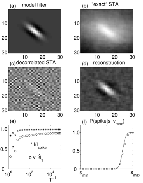
Figure 1: Analysis of a model simple cell with RF shown in (a). The “exact” spike-triggered average ${\bf v}_{\rm\tiny sta}$ is shown in (b). Panel (c) shows an attempt to remove correlations according to reverse correlation method, $C_{a\,priori}^{-1}{\bf v}_{\rm sta}$; (d) vector $\hat{v}_{\rm max}$ found by maximizing information; (e) convergence of the algorithm according to information $I({\bf v})$ and projection $\hat{v}\cdot\hat{e}_{1}$ as a function of inverse effective temperature $T^{-1}$. (f) The probability of a spike $P({\rm spike}|{\bf s}\cdot\hat{v}_{max})$ (crosses) is compared to $P({\rm spike}|s_{1})$ used in generating spikes (solid line). Parameters $\sigma=0.05(s_{\rm max}-s_{\rm min})$ and $s_{t}=0.8(s_{\rm max}-s_{\rm min})$ [$s_{\rm max}$ and $s_{\rm min}$ are the maximum and minimum values of $s_{1}$ over the ensemble of presented stimuli].

The spike–triggered average (STA), or reverse correlation function [9, 21], shown in Fig. 1(b), is broadened because of spatial correlations present in the stimuli. In a model, the effect of noise on our estimate of the STA can be eliminated by averaging the presented stimuli weighted with the exact firing rate, as opposed to using a histogram of responses to estimate $P({\rm spike}|{\bf s})$ from a finite set of trials. We have used this “exact” STA,

$${\bf v}_{\rm sta}=\int d^{D}{\bf s}\,{\bf s}P({\bf s}|{\rm spike})={1\over{P({\rm spike})}}\int d^{D}{\bf s}P({\bf s})\,{\bf s}P({\rm spike}|{\bf s}),$$ (13)

in calculations presented in Fig. 1(bc). If stimuli were drawn from a Gaussian probability distribution, they could be decorrelated by multiplying ${\bf v}_{\rm sta}$ by the inverse of the a priori covariance matrix, according to the reverse correlation method, ${\hat{v}}_{Gaussian\,est}\propto C_{a\,priori}^{-1}{\bf v}_{\rm sta}$. The procedure is not valid for non–Gaussian stimuli and nonlinear input–output functions (1). The result of such a decorrelation is shown in Fig. 1(c). It clearly is missing some of the structure in the model filter, with projection $\hat{e}_{1}\cdot{\hat{v}}_{Gaussian\,est}\approx 0.14$. The discrepancy is not due to neural noise or finite sampling, since the “exact” STA was decorrelated; the absence of noise in the exact STA also means that there would be no justification for smoothing the results of the decorrelation. The discrepancy between the true receptive field and the decorrelated STA increases with the strength of nonlinearity in the input–output function.

In contrast, it is possible to obtain a good estimate of the relevant direction $\hat{e}_{1}$ by maximizing information directly, see panel (d). A typical progress of the simulated annealing algorithm with decreasing temperature $T$ is shown in Fig. 1(e). There we plot both the information along the vector, and its projection on $\hat{e}_{1}$. The final value of projection depends on the size of the data set, see below. In the example shown in Fig. 1 there were $\approx 50,000$ spikes with average probability of spike $\approx 0.05$ per frame, and the reconstructed vector has projection ${\hat{v}}_{max}\cdot\hat{e}_{1}\approx 0.9$. Having estimated the RF, one can proceed to sample the nonlinear input-output function. This is done by constructing histograms for $P({\bf s}\cdot{\hat{v}}_{\rm max})$ and $P({\bf s}\cdot{\hat{v}}_{\rm max}|{\rm spike})$ of projections onto vector $\hat{v}_{\rm max}$ found by maximizing information, and taking their ratio, as in Eq. (2). In Fig. 1(f) we compare $P({\rm spike}|{\bf s}\cdot{\hat{v}}_{\rm max})$ (crosses) with the probability $P({\rm spike}|s_{1})$ used in the model (solid line).

3.2 Estimated deviation from the optimal direction

When information is calculated from a finite data set, the vector ${\bf v}$ which maximizes $I$ will deviate from the true RF $\hat{e}_{1}$. The deviation $\delta{\bf v}={\bf v}-\hat{e}_{1}$ arises because the probability distributions are estimated from experimental histograms and differ from the distributions found in the limit on infinite data size. For a simple cell, the quality of reconstruction can be characterized by the projection ${\bf v}\cdot\hat{e}_{1}=1-\frac{1}{2}\delta{\bf v}^{2}$, where both ${\bf v}$ and $\hat{e}_{1}$ are normalized, and $\delta{\bf v}$ is by definition orthogonal to $\hat{e}_{1}$. The deviation $\delta{\bf v}\sim A^{-1}\nabla I$, where $A$ is the Hessian of information. Its structure is similar to that of a covariance matrix:

$$A_{ij}=\frac{1}{\ln 2}\int dxP(x|{\rm spike})\left(\frac{d}{dx}\ln\frac{P(x|{\rm spike})}{P(x)}\right)^{2}(\langle s_{i}s_{j}|x\rangle-\langle s_{i}|x\rangle\langle s_{j}|x\rangle).$$ (14)

When averaged over possible outcomes of $N$ trials, the gradient of information is zero for the optimal direction. Here in order to evaluate $\langle\delta{\bf v}^{2}\rangle={\rm Tr}[A^{-1}\langle\nabla I\nabla I^{T}\rangle A^{-1}]$, we need to know the variance of the gradient of $I$. By discretizing both the space of stimuli and possible projections $x$, and assuming that the probability of generating a spike is independent for different bins, we estimate $\langle\nabla I_{i}\nabla I_{j}\rangle\sim A_{ij}/(N_{\rm spike}\ln 2)$. Therefore an expected error in the reconstruction of the optimal filter is inversely proportional to the number of spikes and is given by:

$$1-{\bf v}\cdot\hat{e}_{1}\approx\frac{1}{2}\langle\delta{\bf v}^{2}\rangle=\frac{{\rm Tr}[A^{-1}]}{2N_{\rm spike}\ln 2}$$ (15)

In Fig. 2 we plot the average projection of the normalized reconstructed vector ${\bf v}$ on the RF $\hat{e}_{1}$, and show that it scales correctly with the number of spikes.

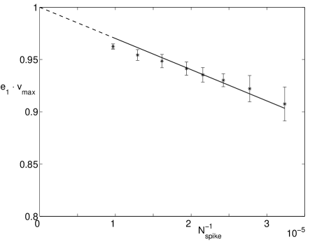
Figure 2: Projection of vector $\hat{v}_{\rm max}$ that maximizes information on RF $\hat{e}_{1}$ is plotted as a function of the number of spikes to show the linear scaling in $1/N_{\rm spike}$. In this series of simulations, the average probability of a spike (12) had parameter values $\sigma=0.1(s_{\rm max}-s_{\rm min})$ and $s_{t}=0.6(s_{\rm max}-s_{\rm min})$.

3.3 A model complex cell

A sequence of spikes from a model cell with two relevant directions was simulated by projecting each of the stimuli on vectors that differ by $\pi/2$ in their spatial phase, taken to mimic properties of complex cells, as in Fig. 3. A particular frame leads to a spike according to a logical OR, that is if either $s_{1}={\bf s}\cdot\hat{e}_{1}$, $-s_{1}$, $s_{2}={\bf s}\cdot\hat{e}_{2}$, or $-s_{2}$ exceeds a threshold value $s_{t}$ in the presence of noise. Similarly to (12),

$$\frac{P({\rm spike}|{\bf s})}{P({\rm spike})}=f(s_{1},s_{2})=\langle\theta(|s_{1}|-s_{t}-\xi_{1})\;\vee\;\theta(|s_{2}|-s_{t}-\xi_{2})\rangle\,,$$ (16)

where $\xi_{1}$ and $\xi_{2}$ are independent Gaussian variables. The sampling of this input–output function by our particular set of natural stimuli is shown in Fig. 3(c). Some, especially large, combinations of values of $s_{1}$ and $s_{2}$ are not present in the ensemble. As is well known, reverse correlation fails in this case because the spike–triggered average stimulus is zero, although with Gaussian stimuli the spike–triggered covariance method would recover the relevant dimensions. Here we show that searching for maximally informative dimensions allows us to recover the relevant subspace even under more natural stimulus conditions.

We start by maximizing information with respect to one direction. Contrary to the result Fig. 1(e) for a simple cell, one optimal direction recovers only about 60% of the total information per spike [Eq. (4)]. Perhaps surprisingly, because of the strong correlations in natural scenes, even projection onto a random vector in the $D\sim 10^{3}$ dimensional stimulus space has a high probability of explaining 60% of total information per spike. We therefore go on to maximize information with respect to two directions. An example of the reconstruction of input–output function of a complex cell is given in Fig. 3. Vectors ${\bf v}_{1}$ and ${\bf v}_{2}$ that maximize $I({\bf v}_{1},{\bf v}_{2})$ are not orthogonal, and are also rotated with respect to $\hat{e}_{1}$ and $\hat{e}_{2}$. However, the quality of reconstruction is independent of a particular choice of basis with the RS. The appropriate measure of similarity between the two planes is the dot product of their normals. In the example of Fig. 3, $\hat{n}_{(\hat{e}_{1},\hat{e}_{2})}\cdot\hat{n}_{({\bf v}_{1},{\bf v}_{2})}\approx 0.8$.

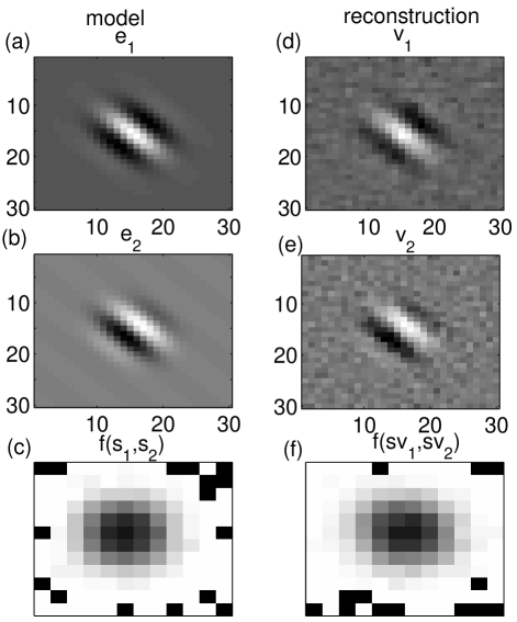
Figure 3: Analysis of a model complex cell with relevant direction $\hat{e}_{1}$ and $\hat{e}_{2}$ shown in (a) and (b). Spikes are generated according to an “OR” input-output function $f(s_{1},s_{2})$ with the threshold $s_{t}=0.6(s_{\rm max}-s_{\rm min})$ and noise variance $\sigma=0.05(s_{\rm max}-s_{\rm min})$. Panel (c) shows how the input-output function is sampled by our ensemble of stimuli. Dark pixels for large values of $s_{1}$ and $s_{2}$ correspond to cases where $P(s_{1},s_{2})=0$. On the right, we show vectors ${\bf v}_{1}$ and ${\bf v}_{2}$ found by maximizing information $I({\bf v}_{1},{\bf v}_{2})$ together with the corresponding input-output function with respect to projections ${\bf s}\cdot{\bf v}_{1}$ and ${\bf s}\cdot{\bf v}_{2}$, panel (f).

Maximizing information with respect to two directions requires a significantly slower cooling rate, and consequently longer computational times. However, the expected error in the reconstruction, $1-\hat{n}_{(\hat{e}_{1},\hat{e}_{2})}\cdot\hat{n}_{({\bf v}_{1},{\bf v}_{2})}$, follows a $N^{-1}_{\rm spike}$ behavior, similarly to (15), and is roughly twice that for a simple cell given the same number of spikes.

4 Remarks

In conclusion, features of the stimulus that are most relevant for generating the response of a neuron can be found by maximizing information between the sequence of responses and the projection of stimuli on trial vectors within the stimulus space. Calculated in this manner, information becomes a function of direction in a stimulus space. Those directions that maximize the information and account for the total information per response of interest span the relevant subspace. This analysis allows the reconstruction of the relevant subspace without assuming a particular form of the input–output function. It can be strongly nonlinear within the relevant subspace, and is to be estimated from experimental histograms. Most importantly, this method can be used with any stimulus ensemble, even those that are strongly non–Gaussian as in the case of natural images.

References

- [1] F. Rieke, D. A. Bodnar, and W. Bialek. Naturalistic stimuli increase the rate and efficiency of information transmission by primary auditory afferents. Proc. R. Soc. Lond. B 262:259–265, 1995.
- [2] F. E. Theunissen, K. Sen, and A. J. Doupe. Spectral-temporal receptive fields of nonlinear auditory neurons obtained using natural sounds. J. Neurosci. 20:2315–2331, 2000.
- [3] W. E. Vinje and J. L. Gallant. Sparse coding and decorrelation in primary visual cortex during natural vision. Science 287:1273–1276, 2000.
- [4] G. D. Lewen, W. Bialek, and R. R. de Ruyter van Steveninck. Neural coding of naturalistic motion stimuli. Network: Comput. Neural Syst. 12:317–329, 2001. See also physics/0103088.
- [5] K. Sen, F. E. Theunissen, and A. J. Doupe. Feature analysis of natural sounds in the songbird auditory forebrain. J. Neurophysiol. 86:1445–1458, 2001.
- [6] N. J. Vickers, T. A. Christensen, T. Baker, and J. G. Hildebrand. Odour-plume dynamics influence the brain’s olfactory code. Nature 410:466–470, 2001.
- [7] W. E. Vinje and J. L. Gallant. Natural stimulation of the nonclassical receptive field increases information transmission efficiency in V1. J. Neurosci. 22:2904–2915, 2002.
- [8] D. L. Ringach, M. J. Hawken, and R. Shapley. Receptive field structure of neurons in monkey visual cortex revealed by stimulation with natural image sequences. Journal of Vision 2:12–24, 2002.
- [9] F. Rieke, D. Warland, R. R. de Ruyter van Steveninck, and W. Bialek. Spikes: Exploring the neural code. MIT Press, Cambridge, 1997.
- [10] E. Simoncelli and B. A. Olshausen. Natural image statistics and neural representation. Annu. Rev. Neurosci. 24:1193-1216, 2001.
- [11] H. B. Barlow. Possible principles underlying the transformation of sensory messages. In Sensory Communication, W. Rosenblith, ed., pp. 217–234 (MIT Press, Cambridge).
- [12] H. B. Barlow. Redundancy reduction revisited. Network: Comput. Neural Syst. 12:241-253, 2001.
- [13] W. Bialek. Thinking about the brain. To be published in Physics of Biomolecules and Cells, H. Flyvbjerg, F. Jülicher, P. Ormos, and F. David, eds. (EDP Sciences, Les Ulis; Springer-Verlag, Berlin 2002). See also physics/0205030.
- [14] T. von der Twer and D. I. A. Macleod. Optimal nonlinear codes for the perception of natural colours. Network: Comput. Neural Syst. 12:395-407, 2001.
- [15] N. Brenner, W. Bialek, and R. de Ruyter van Steveninck. Adaptive rescaling optimizes information transmission, Neuron 26:695–702, 2000.
- [16] A.L. Fairhall, G. D. Lewen, W. Bialek, and R. R. de Ruyter van Steveninck, Efficiency and ambiguity in an adaptive neural code. Nature 412:787–792, 2001.
- [17] Z. F. Mainen and T. J. Sejnowski. Reliability of spike timing in neocortical neurons. Science 268:1503–1506, 1995.
- [18] R. R. de Ruyter van Steveninck, G. D. Lewen, S. P. Strong, R. Koberle, and W. Bialek. Reproducibility and variability in neural spike trains. Science 275:1805–1808, 1997.
- [19] P. Kara, P. Reinagel, and R. C. Reid. Low response variability in simultaneously recorded retinal, thalamic, and cortical neurons. Neuron 27:635–646, 2000.
- [20] R. de Ruyter van Steveninck, A. Borst, and W. Bialek. Real time encoding of motion: Answerable questions and questionable answers from the fly’s visual system. In Processing Visual Motion in the Real World: A Survey of Computational, Neural and Ecological Constraints, J. M. Zanker and J. Zeil, eds., pp. 279–306 (Springer–Verlag, Berlin, 2001). See also physics/0004060.
- [21] E. de Boer and P. Kuyper. Triggered correlation. IEEE Trans. Biomed. Eng. 15:169–179, 1968.
- [22] R. R. de Ruyter van Steveninck and W. Bialek. Real-time performance of a movement-sensitive neuron in the blowfly visual system: coding and information transfer in short spike sequences. Proc. R. Soc. Lond. B 234:379–414, 1988.
- [23] N. Brenner, S. P. Strong, R. Koberle, W Bialek, and R. R. de Ruyter van Steveninck. Synergy in a neural code. Neural Comp. 12:1531-1552, 2000. See also physics/9902067.
- [24] W. Bialek and R. R. de Ruyter van Steveninck. Features and dimensions: Motion estimation in fly vision. In preparation.
- [25] A. Treves and S. Panzeri. The upward bias in measures of information derived from limited data samples. Neural Comp. 7:399-407, 1995.
- [26] S. P. Strong, R. Koberle, R. R. de Ruyter van Steveninck, and W. Bialek. Entropy and information in neural spike trains. Phys. Rev. Lett. 80:197–200, 1998. See also cond-mat/9603127.