Abstract

The effects of the experiment itself upon the obtained results and, especially, the influence of a large number of experiments are extensively discussed in the literature. We show that the important factor that stands at the basis of these effects is that the involved experiments are related and not independent and detached from each other. This relationship takes, as shown here, different forms for different situations and is found in entirely different physical regimes such as the quantum and classical ones.

KEY WORDS: Feynman integrals; Everett’s relative state; entropy; measurement theory

1 Introduction

The effects of observation upon the obtained results have been extensively discussed in the literature (see, for example, [1] and references therein). A special kind of experimentations which attract many discussions by many authors [2, 3, 4, 5, 6] are those in which a large number of experiments are involved. Among these one may note the special role played by those in which the time duration of each of the involved experiments tends to become infinitesimally small. Two quantum versions of these very short-time experiments were studied; (1) The same experiment is infinitely repeated, in a finite total time, upon the same system which results in preserving its initial state (from the very large number of different states to which it may be projected by the experiment) [2, 3, 4]. (2) A very large number of slightly different experiments are densely performed upon the same system which results in "realizing" [5] the path of states through which the system is continuously projected. That is, the probability to be projected to this specific path of states (and not to any of the other large number of different possible paths along which the system may evolute) tends to unity [5, 6]). The first version is termed static Zeno effect and the second dynamic Zeno effect [6].

Another kind of observation that involves many experiments is the space Zeno effect [7] which is obtained when one performs the same experiment in a large number of identical independent nonoverlapping regions of space. It has been shown [7] that when these regions become infinitesimally small, corresponding to the shrinking of the measurement times in the time Zeno effect, the performance of such experiments has, as for the static Zeno, a null effect [7].

We show here that what generally characterizes these and other similar situations is that all the involved experiments, even those that seems to be entirely independent, are related to each other in some kind of relationship which is responsible for the obtained results. This is shown for entirely remote and different physical situations which are studied by different methods such as the Feynman path integral [8], the Everett’s universal wave function [9, 10] and the classical cylinder-piston system [11, 12]. We show that the mentioned relationship assumes different forms for these different situations which, actually, determine the necessary details of the involved experiments. Thus, for some situations, like the static Zeno efect, all the systems should be related by preparing them in the same initial state whereas for the dynamic Zeno effect they are related by preparing them in different initial states as we show in Section 1. We represent in the following sections examples which explain the meaning of this relationship and the effects it produces.

In Section 2 we use the Feynman path integral method [8] to show that if one wants to obtain a large probability for an evolution along a prescribed path of states then all the involved systems must be related so that not even two of them happen to have the same initial state. That is, if this condition is not strictly kept and one prepares these systems so that some of them may have the same initial states then the expected evolution along the specified path of states may not be obtained. In Section 3 we use the Everett’s relative state theory [9, 10], which has been especially formulated to take into account the influence of observers and experiments, to show the effect of experimenting with related systems. In Everett’s theory the necessity of relationship among the systems is so obvious that it becomes almost trivial to emphasize it. We show that if the measurement of the observable $A$ results with $K$ different possible outcomes then the probability to find a specified group of $r$ eigenvalues (from the given $K$) in an $n$-sequence becomes very small for large $K$ and small $r$. This is effected through obtaining an asymptotically large number of different sequences (observers) for these values of $K$ and $r$ which means that the relationship among them is very small.

In Section 4 we use entropy considerations and the classical thermodynamical system of cylinder and pistons [11, 12] to show the influence of related systems. We generalize the discussion in [12] to include a large ensemle of identical cylinders and show that the results obtained when these systems are related greatly differ from those obtained when the ensemble’s components are independent.

2 The Feynman path integrals of the ensemble of observers

The large number of experiments discussed here are performed by first preparing $N$ similar systems at $N$ arbitrarily selected states from, actually, the very large number of possible states which may be assigned to any system. These systems are then delivered to the $N$ observers of the ensemble so that the system $i$ $(i=1,2,\ldots N)$, prepared at the state $\phi_{i}$, is assigned to the observer $O_{i}$. As known [17], the state of any quantum system changes with time without having to touch it. Thus, we may write for the conditional probability of a self-transition that the first observer $O_{1}$ finds his system, after checking its present state, to be at the state $\phi_{2}$ of the second observer $O_{2}$

$$\Phi_{12}=\sum_{i}\phi_{1i}\phi_{i2}$$ (1)

The summation is over all the possible secondary paths [13] (as those shown along the middle path of Figure 1) which lead from $\phi_{1}$ to $\phi_{2}$ and the quantities $\phi_{1i}$ and $\phi_{i2}$ denote [8] the probability amplitudes to proceed from the state $\phi_{1}$ to the intermediate one $\phi_{i}$ and from $\phi_{i}$ to $\phi_{2}$ respectively. In the same manner one may write for the conditional probability amplitude that the second observer $O_{2}$ finds his system at the state $\phi_{3}$ (of the observer $O_{3}$), provided that the observer $O_{1}$ finds his system at the state $\phi_{2}$

$$\Phi_{23|12}=\sum_{ij}\phi_{1i}\phi_{i2}\phi_{2j}\phi_{j3}$$ (2)

Where $\Phi_{23|12}$ is the remarked conditional probability amplitude and $\sum_{ij}$ is the summation over all the secondary paths that lead from the state $\phi_{1}$ to $\phi_{2}$ and over those from $\phi_{2}$ to $\phi_{3}$. Correspondingly, the conditional probability amplitude that the $(N-1)$-th observer finds his system at the state $\phi_{N}$ of the observer $O_{N}$ provided that all the former $(N-2)$ observers find their respective systems to be at the states $\phi_{i}\ \ (i=2,3,\ldots N-1)$ is

$$\Phi_{N-1N|12,23,\ldots,N-2N-1}=\sum_{ij\ldots rs}\phi_{1i}\phi_{i2}\phi_{2j}\phi_{j3}\ldots\phi_{N-2r}\phi_{rN-1}\phi_{N-1s}\phi_{sN},$$ (3)

where the intermediate states in Eqs (1)-(3) are orthonormal. Figure 1 shows 7 Feynman paths of states, from actually a large number of paths, that all begin at the state $\phi_{1}$ and end at $\phi_{8}$ (only 8 states are shown in the figure for clarity). The middle path is the specific one along which the described collective measurement is performed. Along this line we have the $N$ ($N=8$ in the figure) initially prepared states $\phi_{1},\phi_{2},\ldots\phi_{N}$ as well as the secondary Feynman paths that lead from each $\phi_{i}$ to $\phi_{i+1}$ where $i=1,2,\ldots,(N-1)$. As seen from Eqs (1)-(3) the paths (of states) between nonneighbouring states as, for example, from $\phi_{i}$ to $\phi_{i+2}$ are obtained as the sum of the separate paths which lead from $\phi_{i}$ to $\phi_{i+1}$ and from $\phi_{i+1}$ to $\phi_{i+2}$.

The relevant conditional probability is found by multiplying the last probability amplitude from Eq (3) by its conjugate to obtain, omitting the subscripts of the $\Phi$’s for clarity

$$\Phi^{\dagger}\Phi=\sum_{\grave{i}\grave{j}\ldots\grave{r}\grave{s}}\sum_{ij\ldots rs}\phi_{\grave{i}1}\phi_{1i}\phi_{2\grave{i}}\phi_{i2}\phi_{\grave{j}2}\phi_{2j}\phi_{3\grave{j}}\phi_{j3}\ldots\phi_{\grave{r}N-2}\phi_{N-2r}\phi_{N-1\grave{r}}\phi_{rN-1}\cdot$$

$$\cdot\phi_{\grave{s}N-1}\phi_{N-1s}\phi_{N\grave{s}}\phi_{sN}=(\sum_{\grave{i}i}\phi_{\grave{i}1}\phi_{1i}\phi_{2\grave{i}}\phi_{i2})(\sum_{\grave{j}j}\phi_{\grave{j}2}\phi_{2j}\phi_{3\grave{j}}\phi_{j3})\ldots$$ (4)

$$\ldots(\sum_{\grave{r}r}\phi_{\grave{r}N-2}\phi_{N-2r}\phi_{N-1\grave{r}}\phi_{rN-1})(\sum_{\grave{s}s}\phi_{\grave{s}N-1}\phi_{N-1s}\phi_{N\grave{s}}\phi_{sN}),$$

where the number of all the double sums $\sum_{\grave{i}i}\sum_{\grave{j}j}\ldots\sum_{\grave{r}r}\sum_{\grave{s}s}$ is $N$.

As remarked, we are interested in the limit of dense measurement along the relevant Feynman path so we take $N\to\infty$. In this limit the length of the secondary Feynman paths among the initially prepared $N$ states (where now $N\to\infty$) tends to zero [13] so that the former probabilities to proceed along the secondary paths between the given states become the probabilities for these states [13]. Thus, we may write for Eq (4) in the limit of $N\to\infty$

$$\lim_{N\to\infty}<\!\Phi^{\dagger}|\Phi\!>=\lim_{N\to\infty}<\!\phi_{\grave{I}1}|\phi_{2\grave{I}}\!><\!\phi_{I2}|\phi_{1I}\!><\!\phi_{\grave{J}2}|\phi_{3\grave{J}}\!><\!\phi_{J3}|\phi_{2J}\!>\ldots$$

$$\ldots<\!\phi_{\grave{R}(N-2)}|\phi_{(N-1)\grave{R}}\!><\!\phi_{R(N-1)}|\phi_{(N-2)R}\!><\!\phi_{\grave{S}(N-1)}|\phi_{N\grave{S}}\!>\cdot$$ (5)

$$\cdot<\!\phi_{SN}|\phi_{(N-1)S}\!>=\delta_{\phi_{\grave{I}1}\phi_{2\grave{I}}}\delta_{\phi_{1I}\phi_{I2}}\delta_{\phi_{\grave{J}2}\phi_{3\grave{J}}}\delta_{\phi_{2J}\phi_{J3}}\ldots\delta_{\phi_{\grave{R}(N-2)}\phi_{(N-1)\grave{R}}}\cdot$$

$$\cdot\delta_{\phi_{R(N-1)}\phi_{(N-2)R}}\delta_{\phi_{\grave{S}(N-1)}\phi_{N\grave{S}}}\delta_{\phi_{SN}\phi_{(N-1)S}}=1,$$

where the former indices, for finite $N$, $i,{\grave{i}},j,{\grave{j}},\ldots,r,{\grave{r}},s,{\grave{s}}$ are now, in the limit of $N\to\infty$, written in an upper case format. This is to emphasize that, unlike the case for finite $N$, neighbouring states along the traversed Feynman path differ infinitesimally. The last result of unity follows because, as just noted, in the limit of $N\to\infty$ successive states differ infinitesimally from each other so we may write as in [6] $<\!\phi_{\grave{k}-1}|\phi_{\grave{k}}\!>=<\!\phi_{k-1}|\phi_{k}\!>\approx\delta_{\phi_{\grave{k}-1}\phi_{\grave{k}}}=\delta_{\phi_{k-1}\phi_{k}}\approx 1$. Thus, we see that performing dense measurement along any Feynman path of states results in its "realization" [5, 6] in the sense that the probability to proceed through all of its states tends to unity.

As remarked, the key feature of the described dense measurement is that all the $N$ systems are related to each other in such a way that their $N$ initial states are prepared to be different from each other where in the limit of $N\to\infty$ these differences become infinitesimal for neighbouring states. Note that we do not take all the $N$ initial states to be identical since in this case all the former discussion and Eqs (1)-(5) would not be relevant. This is because the primary Feynman path formerly applied for describing the path of these $N$ states would shrink to a point if they are identical. Note that by taking the limit of $N\to\infty$ and by having (for continuity) a slight differences between neighbouring states we have already caused the secondary Feynman paths of the relevant primary one (see Figure 1) to shrink and disappear. Thus, as noted, taking $N$ identical initial states may causes the primary Feynman path, in the limit of $N\to\infty$, to shrink to a point which is not the meant results of this discussion. Note that this procedure of taking $N$ different initial states where the neighbouring ones differ infinitesimally in the limit of $N\to\infty$ is the key property of the dynamic Zeno effect as seen in [5, 6] (see, especially, Sections 1-2 in [6]). Also the continuity condition is not violated as seen from Eq (5).

Note that the described dense measurement is performed through the joint action of all the members of the ensemble as schematically illustrated in Figure 2 which represents the ensemble of observers after the remarked collective measurement. Each batch of 4 similar curves denotes a member of the $N$-ensemble system that has, as known, a large number of different possible Feynman paths of evolution (only 4 are shown for clarity). In the middle part of the figure we have a large number of different batches of paths all mixed among them so it becomes difficult to see which curve belongs to which batch. This corresponds to densely measuring ( $N\to\infty$) where neighbouring states infinitesimally differ from each other. The emphasized path in Figure 2 is the definite path along which the described collective dense measurement has been done. Note that this path, actually, belongs to all the different mixed batches which means that after completing the collective measurement each one of those that participates in it has now the same Feynman path. The reason is that although each observer $O_{i}$ of the ensemble performs his experiment on his prepared state $\phi_{i}$, nevertheless, the results he obtains are valid for all the others since any observer that acts on the same state $\phi_{i}$ under exactly the same conditions obtains the same result. In other words, the emphasized Feynman path belongs now to all of them in the sense that the probability for each to move along its constituent states tends to unity as seen from Eq (5).

We note that in contrast to the relationship discussed just now which demands a preparation of different initial states for the realization of its (dynamic Zeno) effect the situation regarding the static Zeno effect is opposite and contrary. This is because the required relationship there demands to prepare all the initial states of the involved experiments to be identical [2] so as to be able to preserve this state in time. We note that using a large ensemble of similar systems for analysing experimental results has been fruitfully done in the literature [10, 14, 15, 16] without invoking any Zeno idea. It has been shown, for example, that by considering $N$ identical systems all prepared in the same initial state one may derive the probability interpretation of quantum mechanics in the limit of $N\to\infty$. That is, this probability is not imposed upon the theory as an external assumption as done in the conventional Copenhagen interpretation [17] of quantum mechanics but is derived from other principles of quantum mechanics [16]. This is done using Finkelstein theorem [14, 16].

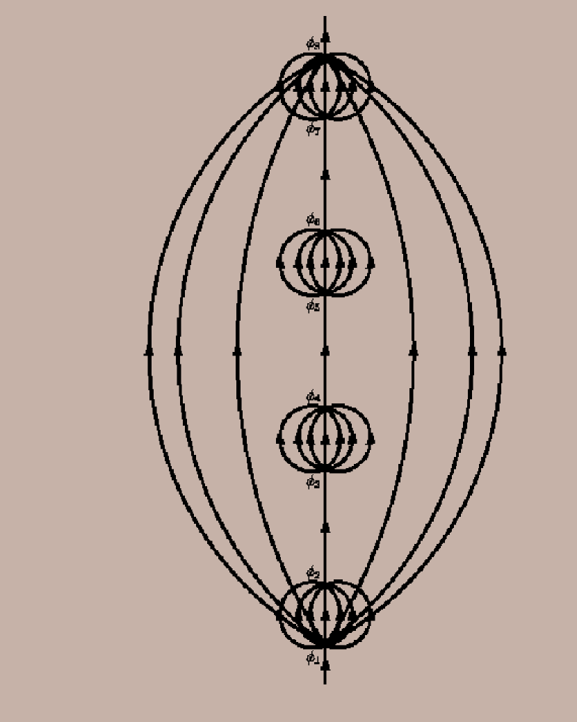
Figure 1: Seven Feynman paths of states, from a very large number of possible ones, that all begin at the state $\phi_{1}$ (at the bottom) and end at $\phi_{8}$ are shown in the figure (only 8 states are shown for clarity). The middle path is the one along which the collective dense measurement is performed by the ensemble members $O_{i},\ \ \ i=1,2,\ldots N$. The $N$ separate systems of these observers have been initially prepared in the states $\phi_{i}\ \ \ i=1,2,\ldots N$. Note the secondary Feynman paths between neighbouring states in the middle path.

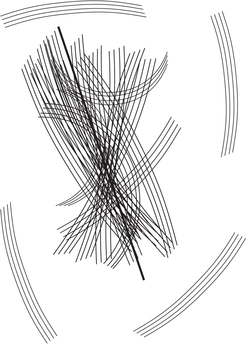
Figure 2: A schematic representation of the physical situation after performing the collective dense measurement symbolized by Figure 1. Note that although no member of the ensemble has done dense measurement by himself, nevertheless, the joint action of all or most of the observers has resulted in “realizing” the specific Feynman path from Figure 1 for all the participating observers. This "realized" path is shown emphasized in the figure.

3 The relative state theory of Everett

The last results may be demonstrated in a more natural and appealing manner by using the relative state theory of Everett [9, 10] which has been formulated, especially, for taking observers into account. We use, in the following, the special notation and terminology of this theory. Thus, if the initial state was some eigenstate of an operator $A$ the total initial state of the (system $S$ $+$ observer $O$) is denoted by $\Psi_{i}^{S+O}=\phi_{i}\Psi^{O}[...]$, where $\phi_{i}$ is the initial eigenstate of the system $S$ and $\Psi^{O}[...]$ denotes the observer’s state before the measurement. After the experiment the observer’s state is denoted by $\Psi^{O}[...\alpha_{i}]$, where $\alpha_{i}$ stands for recording the eigenvalue $\alpha_{i}$ by the observer and the total final state of the (system $S$ $+$ observer $O$) is $\Psi_{f}^{S+O}=\phi_{i}\Psi^{O}[...\alpha_{i}]$. Now, if the initial state of the system is not an eigenstate then it may be expressed as a superpositions of such eigenfunctions $\sum_{i}a_{i}\phi_{i}$ and the total states before and after the measurement are [9, 10] $\Psi_{i}^{S+O}=\sum_{i}a_{i}\phi_{i}\Psi^{O}[...]$, and $\Psi_{f}^{S+O}=\sum_{i}a_{i}\phi_{i}\Psi^{O}[...\alpha_{i}]$ respectively where $a_{i}=<\!\phi_{i}|\Psi^{S+O}\!>$. We note that we consider here the one-step measurement of [9] and not the two-step version [10] of it in which a macroscopic apparatus is introduced between a microscopic system and a macroscopic observer.

We, now, wish to represent the former process of measuring the observable $A$ on $N$ identical independent systems. We assume that the initial state of each one of the $N$ systems is not an eigenstate of $A$ so it can be expanded as a superpositions of such eigenfunctions. Thus, we may write for the initial state of the $N$-system ensemble [9]

$$\Psi_{i}^{S}=\sum_{i}\sum_{j}\cdots\sum_{k}\sum_{l}<\!\phi_{i}|\phi\!><\!\phi_{j}|\phi\!>\ldots<\!\phi_{k}|\phi\!><\!\phi_{l}|\phi\!>\phi_{i}\phi_{j}\ldots\phi_{k}\phi_{l}$$ (6)

where $\phi_{i},\ \ \phi_{j},\ \ldots\phi_{k},\ \ \phi_{l}$ are the eigenfunctions of the operator $A$. Thus, the initial and final states of the total system ($N$ systems $+$ observer) are

$$\Psi_{i}^{S+O}=\sum_{i}\sum_{j}\cdots\sum_{k}\sum_{l}<\!\phi_{i}|\phi\!><\!\phi_{j}|\phi\!>\ldots<\!\phi_{k}|\phi\!><\!\phi_{l}|\phi\!>\phi_{i}\phi_{j}\ldots\phi_{k}\phi_{l}\Psi^{O}[\dots]$$ (7)

$$\Psi_{f}^{S+O}=\sum_{i}\sum_{j}\cdots\sum_{k}\sum_{l}<\!\phi_{i}|\phi\!><\!\phi_{j}|\phi\!>\ldots<\!\phi_{k}|\phi\!><\!\phi_{l}|\phi\!>\phi_{i}\phi_{j}\ldots$$ (8)

$$\ldots\phi_{k}\phi_{l}\Psi^{O}[\alpha_{i},\alpha_{j}\ldots\alpha_{k},\alpha_{l}]$$

where $\Psi^{O}[\alpha_{i},\alpha_{j}\ldots\alpha_{k},\alpha_{l}]$ denotes that the observer has measured the $n$ eigenvalues $\alpha_{i},\alpha_{j}\ldots\alpha_{k},\alpha_{l}$ of $A$. Note that each term in Eq (8) actually denotes an observer with his specific sequence $[\alpha_{i},\alpha_{j}\ldots\alpha_{k},\alpha_{l}]$ which results from the $n$ experiments. Thus, Eq (8), termed the Everett’s universal wave function [9, 10], gives all the possible results that may be obtained from performing the same experiment upon the $n$ systems.

We, now, count the number of observers that have the same or similar sequences $[\alpha_{i},\alpha_{j}\ldots\alpha_{k},\alpha_{l}]$ which record, as remarked, the $n$ measured eigenvalues. For this we assume that each measurement of the observable $A$ may give any of $K$ possible different eigenvalues and that some of the $n$ components in any sequence may be identical. Thus, denoting by $R_{1},R_{2},\ldots,R_{r}$ the numbers of times the $r$ particular different eigenvalues $l_{1},l_{2},\ldots,l_{r}$ respectively appear in some specified sequence $[\alpha_{i},\alpha_{j}\ldots\alpha_{k},\alpha_{l}]$ one may see from Eq (8) that each possible value of $R_{i}$ in the range $0\leq R_{i}\leq n$, and for each $i\ \ \ (1\leq i\leq r)$, may be realized in some observer. Now, the number of sequences in which $l_{1},l_{2},\ldots,l_{r}$ respectively occur at $R_{1},R_{2},\ldots,R_{r}$ predetermined positions is $(K-r)^{(n-\sum_{i=1}^{i=r}R_{i})}$. This is because for each position in the sequence $[\alpha_{i},\alpha_{j}\ldots\alpha_{k},\alpha_{l}]$ in which the $r$ eigenvalues $l_{1},l_{2},\ldots,l_{r}$ are absent there are $(K-r)$ possible locations. Note that $K$ and $r$ should satisfy the relation $K\geq r$. Thus, the total number of sequences in which $l_{1},l_{2},\ldots,l_{r}$ respectively occur in $R_{1},R_{2},\ldots,R_{r}$ positions (we denote this number by $N_{l_{1},l_{2},\ldots,l_{r}}$) is

$$N_{l_{1},l_{2},\ldots,l_{r}}=\left(\begin{array}[]{c}n\\ R_{1}\end{array}\right)\left(\begin{array}[]{c}(n-R_{1})\\ R_{2}\end{array}\right)\left(\begin{array}[]{c}(n-(R_{1}+R_{2}))\\ R_{3}\end{array}\right)\ldots$$ (15)

$$\ldots\left(\begin{array}[]{c}(n-\sum_{i=1}^{i=r-1}R_{i})\\ R_{r}\end{array}\right)(K-r)^{(n-\sum_{i=1}^{i=r}R_{i})},\ \ K\neq r,\ \ K\neq 1$$ (18)

where $\left(\begin{array}[]{c}n\\ R_{1}\end{array}\right)$ is the number of possible ways to choose in the $n$-member sequence $[\alpha_{i},\alpha_{j}\ldots\alpha_{k},\alpha_{l}]$ $R_{1}$ places for $l_{1}$, $\left(\begin{array}[]{c}(n-R_{1})\\ R_{2}\end{array}\right)$ is the number of possible ways to choose $R_{2}$ places from the remaining $(n-R_{1})$ etc. Note that when $K=r$, which means that any one of the $K$ possible results of the experiment must be one of the $r$ eigenvalues $l_{1},l_{2},\ldots,l_{r}$, then the probability that all the $n$ components (where some of them may be identical) of any sequence belong to the $l_{1},l_{2},\ldots,l_{r}$’s group is unity. In this case the number of observers that have in their sequences all the $r$ different eigenvalues $l_{1},l_{2},\ldots,l_{r}$ is

$$N_{l_{1},l_{2},\ldots,l_{r}}=\left(\begin{array}[]{c}n\\ R_{1}\end{array}\right)\left(\begin{array}[]{c}(n-R_{1})\\ R_{2}\end{array}\right)\left(\begin{array}[]{c}(n-(R_{1}+R_{2}))\\ R_{3}\end{array}\right)\ldots\left(\begin{array}[]{c}(n-\sum_{i=1}^{i=r-1}R_{i})\\ R_{r}\end{array}\right),$$

$$K=r,\ \ \ K\neq 1$$

which is the same as Eq (15) but without the factor in $K$.

The relevant measure may be found [10] by taking account of the expected relative frequency $P_{l_{1},l_{2},\ldots,l_{r}}$ of the eigenvalues $l_{1},l_{2},\ldots,l_{r}$ and the corresponding relative frequency $Q_{m\neq l_{1},l_{2},\ldots,l_{r}}$ of any other eigenvalue $m$ different from $l_{1},l_{2},\ldots,l_{r}$. The first is given by $P_{l_{1},l_{2},\ldots,l_{r}}=|\!\!<\!\Psi_{l_{1},l_{2},\ldots,l_{r}}|\Psi\!>\!\!|^{2}$ where $|\Psi_{l_{1},l_{2},\ldots,l_{r}}\!>$ is the state in which the eigenvalues $l_{1},l_{2},\ldots,l_{r}$ occur among those of the sequence $[\alpha_{i},\alpha_{j}\ldots\alpha_{k},\alpha_{l}]$ and the second is $Q_{m\neq l_{1},l_{2},\ldots,l_{r}}=\sum_{(m\neq l_{1},l_{2},\ldots,l_{r})}|\!\!<\!\Psi_{m\neq l_{1},l_{2},\ldots,l_{r}}|\Psi\!>\!\!|^{2}=1-P_{l_{1},l_{2},\ldots,l_{r}}$ were $|\Psi_{m\neq l_{1},l_{2},\ldots,l_{r}}\!>$ is the state in which the eigenvalues $l_{1},l_{2},\ldots,l_{r}$ do not occur among those of this sequence. Thus, the measure of the sequences that have the eigenvalues $l_{1},l_{2},\ldots,l_{r}$ at the respective $R_{1},R_{2},\ldots,R_{r}$ predetermined positions is $P_{l_{1},l_{2},\ldots,l_{r}}^{\sum_{i=1}^{i=r}R_{i}}Q_{m\neq l_{1},l_{2},\ldots,l_{r}}^{(n-\sum_{i=1}^{i=r}R_{i})}$. The last expression must be multiplied by the number of possible ways to choose first $R_{1}$ places for $l_{1}$ from the $n$ positions of the sequence $[\alpha_{i},\alpha_{j}\ldots\alpha_{k},\alpha_{l}]$, then to choose $R_{2}$ places for $l_{2}$ from the remaining $n-R_{1}$ etc, until the last step of choosing $R_{r}$ places from $(n-\sum_{i=1}^{i=r-1}R_{i})$ (see Eq (15)). That is, the sought-for measure $M_{e}$ is

$$M_{e}(r)=\left(\begin{array}[]{c}n\\ R_{1}\end{array}\right)\left(\begin{array}[]{c}(n-R_{1})\\ R_{2}\end{array}\right)\left(\begin{array}[]{c}(n-(R_{1}+R_{2}))\\ R_{3}\end{array}\right)\ldots$$ (26)

$$\ldots\left(\begin{array}[]{c}(n-\sum_{i=1}^{i=r-1}R_{i})\\ R_{r}\end{array}\right)P_{l_{1},l_{2},\ldots,l_{r}}^{\sum_{i=1}^{i=r}R_{i}}Q_{m\neq l_{1},l_{2},\ldots,l_{r}}^{(n-\sum_{i=1}^{i=r}R_{i})},$$ (29)

which is the Bernoulli distribution [18]. As remarked in [10] $M_{e}(r)$ from Eq (26) may be approximated, for large $N$, by a Gaussian distribution with mean $NP_{l_{1},l_{2},\ldots,l_{r}}$ and standard deviation $\sqrt{NP_{l_{1},l_{2},\ldots,l_{r}}Q_{m\neq l_{1},l_{2},\ldots,l_{r}}}$. We, now, calculate an explicit expression for $P_{l_{1},l_{2},\ldots,l_{r}}(r)$ and $Q_{m\neq l_{1},l_{2},\ldots,l_{r}}(r)$ as functions of $r$, for $n=30$. The probability $P_{l_{1},l_{2},\ldots,l_{r}}(r)$ to find the eigenvalues $l_{1},l_{2},\ldots,l_{r}$ among those of the sequence $[\alpha_{i},\alpha_{j}\ldots\alpha_{k},\alpha_{l}]$ may be written as $P_{l_{1},l_{2},\ldots,l_{r}}(r)=|<\!\Psi_{l_{1},l_{2},\ldots,l_{r}}|\Psi\!>|^{2}=\frac{r}{n}=\frac{r}{30}$, and the probability to find any other eigenvalue $m\neq l_{1},l_{2},\ldots,l_{r}$ is $Q_{m\neq l_{1},l_{2},\ldots,l_{r}}(r)=\sum_{(m\neq l_{1},l_{2},\ldots,l_{r})}|<\!\Psi_{m\neq l_{1},l_{2},\ldots,l_{r}}|\Psi\!>|^{2}=1-P_{l_{1},l_{2},\ldots,l_{r}}=1-\frac{r}{30}=\frac{(30-r)}{30}$. For simplifying the following calculations we assign to all the values of $R_{i}\ \ i=1,2,\ldots r$ the unity value, in which case each of the given eigenvalues $l_{1},l_{2},\ldots,l_{r}$ may occurs only once in the sequence $[\alpha_{i},\alpha_{j}\ldots\alpha_{k},\alpha_{l}]$. Thus, the relevant total number of sequences (observers) $N_{l_{1},l_{2},\ldots,l_{r}}(K,r)$ and the corresponding measure $M_{e}(r)$ from Eqs (15)-(26) are given by

$$N_{l_{1},l_{2},\ldots,l_{r}}(K,r)=\left(\begin{array}[]{c}30\\ 1\end{array}\right)\left(\begin{array}[]{c}29\\ 1\end{array}\right)\ldots\left(\begin{array}[]{c}(30-(r-1))\\ 1\end{array}\right)\cdot$$ (36)

$$\cdot(K-1)^{(30-r)}=\prod_{i=0}^{i=r-1}(30-i)(K-1)^{(30-r)}$$

and

$$M_{e}(r)=\left(\begin{array}[]{c}30\\ 1\end{array}\right)\left(\begin{array}[]{c}29\\ 1\end{array}\right)\ldots\left(\begin{array}[]{c}(30-(r-1))\\ 1\end{array}\right)(\frac{r}{30})^{r}\cdot$$ (43)

$$\cdot(\frac{(30-r)}{30})^{(30-r)}=\prod_{i=0}^{i=r-1}(30-i)(\frac{r}{30})^{r}(\frac{(30-r)}{30})^{(30-r)}$$

Table 1: The table shows the number of observers that have $r$ positions in their 30 places sequences occupied by the preassigned eigenvalues, where the numbers $K$ of possible values for each experiment are 1100, 100, 10, 5 and 2. The untabulated places for $K=10$, $K=5$ and $K=2$ are when $K\leq r$.

r	Number   of	Number   of	Number   of	Number   of	Number   of
	observers for	observers for	observers for	observers for	observers for
	K=1100	K=100	K=10	K=5	K=2
$1$	$4.6350491\cdot 10^{89}$	$2.2415163\cdot 10^{59}$	$1.4130386\cdot 10^{29}$	$8.6469113\cdot 10^{18}$	$3\cdot 10^{1}$
$2$	$1.1922979\cdot 10^{88}$	$4.9413927\cdot 10^{58}$	$1.6828247\cdot 10^{28}$	$1.9902809\cdot 10^{16}$	870
$3$	$2.9665811\cdot 10^{86}$	$1.0703212\cdot 10^{58}$	$1.6007531\cdot 10^{27}$	$3.2695439\cdot 10^{12}$	$---$
$4$	$7.1304257\cdot 10^{84}$	$2.2755852\cdot 10^{57}$	$1.1219501\cdot 10^{26}$	$6.5772\cdot 10^{5}$	$---$
$5$	$1.6533598\cdot 10^{83}$	$4.7435614\cdot 10^{56}$	$5.0964117\cdot 10^{24}$	$171\cdot 10^{5}$	$---$
$6$	$3.6929220\cdot 10^{81}$	$9.6832889\cdot 10^{55}$	$1.2033562\cdot 10^{23}$	$---$	$---$
$7$	$7.9328524\cdot 10^{79}$	$1.9331852\cdot 10^{55}$	$9.6594968\cdot 10^{20}$	$---$	$---$
$8$	$1.6360310\cdot 10^{78}$	$3.7689961\cdot 10^{54}$	$9.8981353\cdot 10^{17}$	$---$	$---$
$9$	$3.2332250\cdot 10^{76}$	$7.1644920\cdot 10^{53}$	$5.1917786\cdot 10^{12}$	$---$	$---$
$10$	$6.1103406\cdot 10^{74}$	$1.3255181\cdot 10^{53}$	$1.09027\cdot 10^{14}$	$---$	$---$
$11$	$1.1017807\cdot 10^{73}$	$2.3821855\cdot 10^{52}$	$---$	$---$	$---$
$12$	$1.890772\cdot 10^{71}$	$4.1496088\cdot 10^{51}$	$---$	$---$	$---$
$13$	$3.0795964\cdot 10^{69}$	$6.9890614\cdot 10^{50}$	$---$	$---$	$---$
$14$	$4.7458902\cdot 10^{67}$	$1.1350519\cdot 10^{50}$	$---$	$---$	$---$
$15$	$6.8961474\cdot 10^{65}$	$1.771921\cdot 10^{49}$	$---$	$---$	$---$
$16$	$9.4115613\cdot 10^{63}$	$2.6494866\cdot 10^{48}$	$---$	$---$	$---$
$17$	$1.2010185\cdot 10^{62}$	$3.7791572\cdot 10^{47}$	$---$	$---$	$---$
$18$	$1.4257725\cdot 10^{60}$	$5.1178711\cdot 10^{46}$	$---$	$---$	$---$
$19$	$1.5652618\cdot 10^{58}$	$6.5439439\cdot 10^{45}$	$---$	$---$	$---$
$20$	$1.5781003\cdot 10^{56}$	$7.8486852\cdot 10^{44}$	$---$	$---$	$---$
$21$	$1.4490723\cdot 10^{54}$	$8.7607415\cdot 10^{43}$	$---$	$---$	$---$
$22$	$1.1997469\cdot 10^{52}$	$9.0135604\cdot 10^{42}$	$---$	$---$	$---$
$23$	$8.8458478\cdot 10^{49}$	$8.4462633\cdot 10^{41}$	$---$	$---$	$---$
$24$	$5.7174346\cdot 10^{47}$	$7.0991954\cdot 10^{40}$	$---$	$---$	$---$
$25$	$3.1733732\cdot 10^{45}$	$5.2454789\cdot 10^{39}$	$---$	$---$	$---$
$26$	$1.4705031\cdot 10^{43}$	$3.3141771\cdot 10^{38}$	$---$	$---$	$---$
$27$	$5.4614504\cdot 10^{40}$	$1.7197979\cdot 10^{37}$	$---$	$---$	$---$
$28$	$1.5241217\cdot 10^{38}$	$6.8753541\cdot 10^{35}$	$---$	$---$	$---$
$29$	$2.8408581\cdot 10^{35}$	$1.8832953\cdot 10^{34}$	$---$	$---$	$---$
$30$	$2.6525286\cdot 10^{32}$	$2.6525286\cdot 10^{32}$	$---$	$---$	$---$

In Table 1 we show the number of observers (sequences) that have $r$ predetermined different eigenvalues in their respective $n$-place sequences for $n=30$ and for the five different values of $K=1100,100,10,5,2$. Note that for the large values of $K$, which signifies a large number of possible results for the measurement of the observable $A$, the sequences most frequently encountered are, as expected, the ones that contain small number of the $r$ eigenvalues. That is, the larger is $K$ the smaller is the relationship among the ensemble’s members. For example, for $K=1100$ and $K=100$ the number of different observers (sequences) with $r=1$, that have only one of the preassigned eigenvalues, are $4.6350491\cdot 10^{89}$ and $2.2415163\cdot 10^{59}$ respectively compared to $2.6525286\cdot 10^{32}$ and $2.6525286\cdot 10^{32}$ that have all the 30 places in their sequences occupied by such eigenvalues. That is, for $K=1100$ and $K=100$ the number of different observers (sequences) with $r=1$ are respectively larger by the factors of $1.7474\cdot 10^{57}$ and $8.45048\cdot 10^{26}$ compared to those with $r=30$.

These results, although in a smaller scale, are found also for small $K$ which signifies a small number of possible different results for the measurement of $A$. That is, most observers are found to have in their sequences a small number of the $r$ predetermined eigenvalues. Note that for small $K$ we can read from Table 1 the values of $N_{l_{1},l_{2},\ldots,l_{r}}$ also for $K=r$. For example, for $K=r=2$ the number of different sequences is greater by a factor of 29 than for $K=2$ and $r=1$. The results of Table 1 are corroborated by directly calculating the relative rate $R(K,r)$ of the increase of $N_{l_{1},l_{2},\ldots,l_{r}}$ from Eq (36) which is

$$R(K,r)=\frac{N_{l_{1},l_{2},\ldots,l_{r}}(K,r)-N_{l_{1},l_{2},\ldots,l_{r}}(K,r-1)}{N_{l_{1},l_{2},\ldots,l_{r}}(K,r)},$$ (44)

It has been found that the rate $R(K,r)$ is always negative for the order of magnitudes of $K=100$ and $r\leq K$ discussed here which means that $N_{l_{1},l_{2},\ldots,l_{r}}(K,r)<N_{l_{1},l_{2},\ldots,l_{r}}(K,r-1)$. That is, as we have found from Table 1, the large number of observers (sequences) are found at small $r$. Also, we find for small $r$ (not shown) that the larger $K$ becomes the more inclined toward negative values is the surface of $R(K,r)$ which means that the large number of observers are found, as in Table 1, at large $K$ and small $r$. When $K=1$, which means that there is only one result for the measurement of $A$, then we must have $r=1$ and the former problem of calculating the probability to find $r$ specified eigenvalues in $n$-sequence reduces to finding one known eigenvalue which is trivially unity since there exists no other eigenvalue to measure.

In summary, we see that an important necessary aspect for obtaining a large probability for a specific configuration of $n$-sequence is that its components must be related. This relationship is expressed through the number of different sequences in Table 1 so that the smaller is this number the greater is the relationship and vice versa. The number of different sequences (observers) is determined by $K$ and $r$ so that for small $K$ and large $r$, where always $K\geq r$, this number is small and for large $K$ and small $r$ it is large. Note that if they do not measure the same observable then the observers are totally unrelated and our former results would not be obtained even for small $K$.

4 The classical effect of an ensemble of observers

We discuss now the same system used in [12] for demonstrating the effect of observation upon the experimental results. The discussion in [12] is generalized to include the large ensemble of related $N$ thermodynamical systems, of the kind studied in [12]. That is, a hollow cylinder that contains $n$ particles, not all of the same kind, among four pistons as shown in Figure 3. The pistons $A$ and $\grave{A}$ are fixed while $B$ and $\grave{B}$ may move along the cylinder. Also the pistons $\grave{A}$ and $B$ do not allow passage of particles through them, whereas $A$ and $\grave{B}$ are permeable so that each permits some kind of particles to move through it where those that are allowed to pass through $A$ are not allowed through $\grave{B}$ and vice versa. The pistons $B$ and $\grave{B}$ move in such a way that the distances $B\grave{B}$ and $A\grave{A}$ are always equal as seen in Figure 3. These distances are measured using the $x$ axis which is assumed to be upward along the cylinder. We assume that the piston $A$ is permeable only to the particles inside the interval $(x_{1},x_{2})$ and $\grave{B}$ only to those outside it. We denote by $w_{1}$ the initial probability that any randomly selected particle is found to be in the interval $(x_{1},x_{2})$ and by $w_{2}$ that it is outside it. At first the pistons $B$ and $\grave{B}$ were at the positions of $A$ and $\grave{A}$ respectively and all the $n$ particles were in the one space between. We, now, wish to perform, reversibly and with no external force, a complete cycle of first moving up the pistons $B\grave{B}$ and then retracing them back to their initial places. Thus, by moving up, without doing work, the pistons $B$ and $\grave{B}$ the volume enclosed between them equals, as remarked, that between $A\grave{A}$ and we obtain two separate equal volumes, each of which equals to the initial one. Now, since $A$ is permeable to the particles in the interval $(x_{1},x_{2})$ and $\grave{B}$ to the rest the result is that the upper volume $B\grave{B}$ contains only the particles from the predetermined interval $(x_{1},x_{2})$ and the lower $A\grave{A}$ only the others.

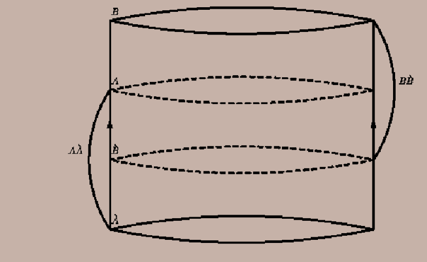
Figure 3: The cylinder with the four pistons. The pistons $A$ and $\grave{A}$ are fixed whereas $B$ and $\grave{B}$ may move along the cylinder. Also the piston $A$ is permeable to the molecules inside the interval $(x_{1},x_{2})$ (see text) and $\grave{B}$ to those outside it.

When we retrace the former steps and move down the pistons $B$ and $\grave{B}$ to their former places at $A$ and $\grave{A}$ the same initial volume is obtained. We must take into account, however, that during the upward motion some particles that were inside (outside) the interval $(x_{1},x_{2})$ may come out of (into) it due to thermal or other kind of fluctuation so that these particles change from the kind that may pass through the piston $A$ ($\grave{B}$) into the kind that is not allowed to do that. Thus, the last step of retracing the pistons $B$, $\grave{B}$ into their former initial positions at the pistons $A$, $\grave{A}$ respectively can not be performed without doing work since the molecules that have come out of (into) the interval $(x_{1},x_{2})$ are not permitted now to pass through $A$ ($\grave{B}$). That is, the former process of expanding the volume is not reversible as described because we have to exert force on these molecules to move them back into (out of) the interval $(x_{1},x_{2})$ so that they can pass through $A$ ($\grave{B}$).

We may express this quantitatively by noting that there is now [12] a decrease of entropy per molecule after the first step of moving up the pistons. This is calculated by taking into account that now the probabilities to find any randomly selected molecule out of (in) the preassigned interval $(x_{1},x_{2})$ are different from the initial values $w_{2}$ and $w_{1}$ before moving up the pistons. Thus, suppose that during the first stage of expanding the initial volume of the cylinder $n_{o}$ molecules, from the total number $n$, have come out of the remarked interval and $n_{i}$ from outside have entered so that the probability to find now any randomly selected molecule out of it is $(w_{2}+\frac{(n_{o}-n_{i})}{n})$ and that to find it in is $(w_{1}+\frac{(n_{i}-n_{o})}{n})$. Thus, denoting the entropies per molecule before and after moving up the pistons by $s_{i}$ and $s_{m}$ respectively we have [12]

$$s_{i}=-k(w_{1}\ln w_{1}+w_{2}\ln w_{2}),$$ (45)

$$s_{m}=-k((w_{1}+\frac{(n_{i}-n_{o})}{n})\ln(w_{1}+\frac{(n_{i}-n_{o})}{n})+$$ (46)

$$+(w_{2}+\frac{(n_{o}-n_{i})}{n})\ln(w_{2}+\frac{(n_{o}-n_{i})}{n})),$$

where $k$ is Boltzman’s constant. The difference in the entropy per molecule between the two situations from Eqs (45)- (46) is

$$\delta s=(s_{m}-s_{i})=-(kw_{1}(\ln(w_{1}+\frac{(n_{i}-n_{o})}{n})-\ln w_{1})+kw_{2}(\ln(w_{2}+$$

$$+\frac{(n_{o}-n_{i})}{n})-\ln w_{2})+k\frac{(n_{o}-n_{i})}{n}(\ln(w_{2}+\frac{(n_{o}-n_{i})}{n})-$$ (47)

$$-\ln(w_{1}+\frac{(n_{i}-n_{o})}{n})))=-(kw_{1}(1+\frac{(n_{i}-n_{o})}{w_{1}n})\ln(1+\frac{(n_{i}-n_{o})}{w_{1}n})+$$

$$+kw_{2}(1+\frac{(n_{o}-n_{i})}{w_{2}n})\ln(1+\frac{(n_{o}-n_{i})}{w_{2}n})+\frac{k(n_{o}-n_{i})}{n}\ln(\frac{w_{2}}{w_{1}}))$$

Eliminating $w_{2}$ through use of the relation $w_{1}+w_{2}=1$ one may write the last equation as

$$\delta s=(s_{m}-s_{i})=-(kw_{1}(1-\frac{(n_{o}-n_{i})}{nw_{1}})\ln(1-\frac{(n_{o}-n_{i})}{nw_{1}})+$$ (48)

$$+k(1-w_{1})(1+\frac{(n_{o}-n_{i})}{n(1-w_{1})})\ln(1+\frac{(n_{o}-n_{i})}{n(1-w_{1})})+\frac{k(n_{o}-n_{i})}{n}\ln(\frac{(1-w_{1})}{w_{1}}))$$

We note that the probability $w_{1}$ must be directly proportional to the length of the remarked interval $x_{2}-x_{1}$, so that a small or large value for one indicates a corresponding value for the other. Thus, we may assume a normal distribution [18] for $w_{1}$ in terms of $x$ and write for the density function of $w_{1}(x)$ $f_{w_{1}}(x)=\frac{\exp(-\frac{(x-\mu)^{2}}{2\sigma^{2}})}{\sqrt{2\pi}\sigma}$, where $\mu$ is the mean value of $x$ and $\sigma$ is the standard deviation. To further simplify the following calculation we assume a standard normal distribution [18] $z=\frac{(x-\mu)}{\sigma}$ for which $\mu=0$ and $\sigma=1$. Thus, the density function $f_{w_{1}}(x)$ may be written as $f_{w_{1}}(z)=\frac{\exp(-\frac{(z)^{2}}{2})}{\sqrt{2\pi}}$ and the probability $w_{1}(x)$ to find any randomly selected molecule in the interval $(-x,x)$, where now this interval is symmetrically located around the origin $x=0$, is [18]

$$w_{1}(x)=\int_{-x}^{x}f_{w_{1}}(z)dz=\frac{1}{\sqrt{2\pi}}\int_{-x}^{x}dze^{-\frac{z^{2}}{2}}=erf(\frac{x}{\sqrt{2}})$$ (49)

$erf(x)$ is the error function defined as $erf(x)=\frac{2}{\sqrt{\pi}}\int_{0}^{x}e^{-u^{2}}du$. Note that $erf(0)=0$, $erf(\infty)=1$, and $erf(-x)=-erf(x)$ so that this function is appropriate for a representation of the probability $w_{1}(x)$. Substituting from Eq (49) into Eq (48) we obtain

$$\delta s=(s_{m}-s_{i})=-(k\cdot erf(\frac{x}{\sqrt{2}})(1-\frac{(n_{o}-n_{i})}{n\cdot erf(\frac{x}{\sqrt{2}})})\ln(1-\frac{(n_{o}-n_{i})}{n\cdot erf(\frac{x}{\sqrt{2}})})+$$

$$+k(1-erf(\frac{x}{\sqrt{2}}))(1+\frac{(n_{o}-n_{i})}{n(1-erf(\frac{x}{\sqrt{2}}))})\ln(1+\frac{(n_{o}-n_{i})}{n(1-erf(\frac{x}{\sqrt{2}}))})+$$ (50)

$$+\frac{k(n_{o}-n_{i})}{n}\ln(\frac{(1-erf(\frac{x}{\sqrt{2}}))}{erf(\frac{x}{\sqrt{2}})}))$$

Eq (50) which gives the entropy decrease per molecule, must be multiplied by the number $n$ of molecules in the cylinder in order to obtain the total decrease of entropy after moving up the pistons. Figure 4 shows a three-dimensional representation of the entropy $s$ per molecule from the last equation as function of $\frac{n_{i}}{n}$ and $\frac{n_{o}}{n}$ which are respectively the fractions of molecules that have entered and come out of the interval $(x_{1},x_{2})$. The probability $w_{1}=erf(\frac{x}{\sqrt{2}})$ must begin from the minimum value of $\frac{n_{0}}{n}$ since $w_{1}$ can not be smaller than $\frac{n_{0}}{n}$. The ranges of both $\frac{n_{i}}{n}$ and $\frac{n_{o}}{n}$ are specified to $0.005\leq\frac{n_{i}}{n},\frac{n_{o}}{n}\leq 0.5$ because in the reversible motion discussed here it is unexpected that more than half of the total particles will enter or leave the interval $(x_{1},x_{2})$. One may realize from the figure that for large values of $\frac{n_{0}}{n}$ ($\frac{n_{i}}{n}$) and comparatively small values of $\frac{n_{i}}{n}$ ($\frac{n_{o}}{n}$) the entopy differences tend to $+1$ ($-1$) and when both $\frac{n_{0}}{n}$ and $\frac{n_{i}}{n}$ are large $s$ tends to zero from negative values.

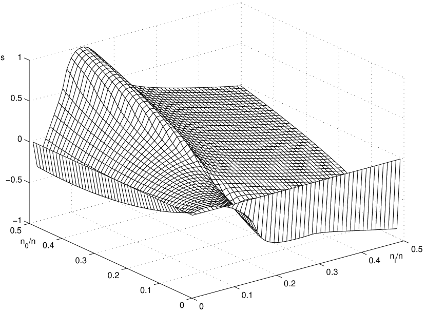
Figure 4: The figure shows a three-dimensional surface of the entropy per molecule $s$ from Eq (50) as function of $\frac{n_{o}}{n}$ and $\frac{n_{i}}{n}$. Both ranges of $\frac{n_{o}}{n}$ and $\frac{n_{i}}{n}$ are $(0.005,0.5)$ since it is unexpected that in a reversible motion more than half of the total molecules will leave or enter the given interval $(x_{1},x_{2})$. Note that for large $\frac{n_{o}}{n}$ ($\frac{n_{i}}{n}$) and small $\frac{n_{i}}{n}$ ($\frac{n_{o}}{n}$) $s$ tends to $+1$ $(-1)$.

As realized from Eq (50) when $n_{o}=n_{i}$, which means that there is no net transfer of molecules out of or into the interval $(x_{1},x_{2})$, the entropy decrease from Eqs (50) is obviously zero. When, however, $n_{o}\neq n_{i}$ the molecules that come out of the interval $(x_{1},x_{2})$ and those that have entered it prevent, as remarked, the reversible return of the pistons to their former places. This problem has been discussed and solved in [12] for the single cylinder. Our main interest is to generalize from this four-piston cylinder to a large ensemble of such cylinders and calculate, as done for the quantum examples in Sections II-III, the correlation among them.

We assume that the initial state of all the $N$ identical four-pistons cylinders is that in which the movable pistons ${\grave{B}_{j}}$, $B_{j}$ are on the fixed ones ${\grave{A}_{j}}$ and $A_{j}$ where $1\leq j\leq N$ (see Figure 3). One then simultaneously and reversibly raise up and down in a complete cycle all the $2N$ movable pistons ${\grave{B}_{j}}$ and $B_{j}$, $1\leq j\leq N$. Thus, if after the moving-up stage we find, for some of them, that no molecule comes out of the interval $(x_{1},x_{2})$ and no one from outside has entered it then, as remarked, they record no entropy decrease during this stage. Note that if no entropy decrease has been detected during the reversible upward motion then one may assume no such decrease also in the downward motion. If, on the other hand, one finds $n_{o}$ molecules come out of the interval $(x_{1},x_{2})$ and $n_{i}$ have entered where $n_{o}\neq n_{i}$ then, as remarked, a decrease of entropy must occurs. In such case the total decrease of entropy for the $N$ cylinders after the moving-up stage is

$$\delta s_{total}=-k\sum_{j=1}^{j=N}n(erf(\frac{x_{j}}{\sqrt{2}})(1-$$ (51)

$$-\frac{(n_{o_{j}}-n_{i_{j}})}{n\cdot erf(\frac{x_{j}}{\sqrt{2}})})\ln(1-\frac{(n_{o_{j}}-n_{i_{j}})}{n\cdot erf(\frac{x_{j}}{\sqrt{2}})})+(1-erf(\frac{x_{j}}{\sqrt{2}}))(1+\frac{(n_{o_{j}}-n_{i_{j}})}{n(1-erf(\frac{x_{j}}{\sqrt{2}}))})\cdot$$

$$\cdot\ln(1+\frac{(n_{o_{j}}-n_{i_{j}})}{n(1-erf(\frac{x_{j}}{\sqrt{2}}))})+\frac{(n_{o_{j}}-n_{i_{j}})}{n}\ln(\frac{(1-erf(\frac{x_{j}}{\sqrt{2}}))}{erf(\frac{x_{j}}{\sqrt{2}})})),$$

where we use Eq (50) and assume that the total number of molecules $n$ are the same for all the ensemble members. We, now, show that when the $N$ experiments of reversibly moving the pistons up and down are related to each other in the sense that no two of them share the same value of either $\frac{n_{o_{j}}}{n}$ or $\frac{n_{i_{j}}}{n}$ (or $x_{j}$), where $1\leq j\leq N$, then the larger is $N$ the more probable is to obtain entropy decrease. If, on the other hand, they are not related in this manner so that some systems share the values of either $\frac{n_{o_{j}}}{n}$ or $\frac{n_{i_{j}}}{n}$ (or $x_{j}$) then the mentioned probability will be discontinuous, stochastic and much less clear compared to the former case. We first note that since for all $x\geq 3$ $erf(x)\approx 1$ we may assume a range of $(-3,3)$ from which we take the values for the $N$ preassigned intervals $(-x_{j},x_{j})$ where $1\leq j\leq N$. That is, we subdivide the interval $(-3,3)$ into $N$ different subintervals, where $N$ is the number of cylinders, so that each has its unique interval $(-x_{j},x_{j})$ besides its specific values of $\frac{n_{o_{j}}}{n}$ and $\frac{n_{i_{j}}}{n}$. Also, each probability $w_{i_{j}}=erf(\frac{x_{j}}{\sqrt{2}})$ for any system $O_{j},\ \ (j=1,2,\ldots,N)$ must begin, as remarked after Eq (50), from the minimum value of $\frac{n_{o_{j}}}{n}$ and we also assume (see the discussion after Eq (50)) that the $2N$ different values of $\frac{n_{i_{j}}}{n}$ and $\frac{n_{o_{j}}}{n}$, $1\leq j\leq N$ are from the range $0.005\leq\frac{n_{o_{j}}}{n},\frac{n_{i_{j}}}{n}\leq 0.5$. We assign to each experiment that results in entropy decrease, after moving-up the pistons, the value of $+1$ and 0 otherwise. Thus, assuming that the movable pistons in the $N$ cylinders are moved up we calculate the quantity

$$g(N)=\frac{1}{N}\sum_{i=1}^{i=N}g_{i}(N),$$ (52)

where $g_{i}(N)=1$ for an entropy decrease result and $g_{i}(N)=0$ otherwise. That is, the function $g(N)$ is directly proportional to the number of experiments which result in entropy decrease and inversely proportional to those with a different result (for which $\delta s\geq 0$). Figure 5 shows $g(N)$ as a function of $N$, in the range $400\leq N\leq 3500$, and we see that $g(N)$ grows as the number $N$ of related cylinders increases where this relationship is effected, as remarked, by preparing the $N$ experiments so that any one of them have its unique $\frac{n_{o_{j}}}{n}$, $\frac{n_{i_{j}}}{n}$ and $(-x_{j},x_{j})$ where $1\leq j\leq N$. That is, the larger is the number of related experiments the more frequent is the result of entropy decrease. If, on the other hand, this kind of relationship is absent as when assigning randomly to any system $O_{j}\ \ (j=1,2,\ldots,N)$ an interval $(-x_{j},x_{j})$ (from $(-3,3)$) and also $\frac{n_{o_{j}}}{n}$, $\frac{n_{i_{j}}}{n}$ (from $(0.005,0.5)$) we obtain a stochastic result for $g(N)$ that implies no clear-cut consistent value. This is clearly seen in the sawtooth form of the curve of Figure 6 which is drawn under exactly the same conditions as those of Figure 5 except that the values of $(-x_{j},x_{j})$, $\frac{n_{o_{j}}}{n}$ and $\frac{n_{i_{j}}}{n}$ are randomly chosen.

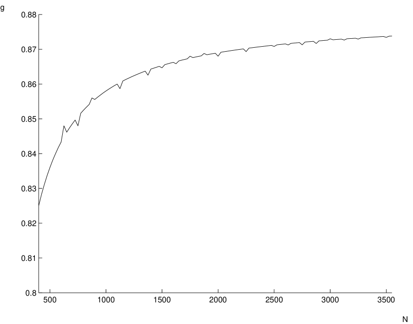
Figure 5: The curve shows the form of $g(N)$ from Eq (52) as a function of $N$ after performing the $N$ experiments of lifting up the pistons where $400\leq N\leq 3500$. Note that no two of the $N$ experiments are identical and that each is deliberately performed for different values of $(-x_{j},x_{j})$, $\frac{n_{o_{j}}}{n}$ and $\frac{n_{i_{j}}}{n}$ where $x_{j}=6\cdot\frac{n_{o_{j}}}{n}$. We see that as $N$ grows the number of experiments that end in an entropy decrease increases.

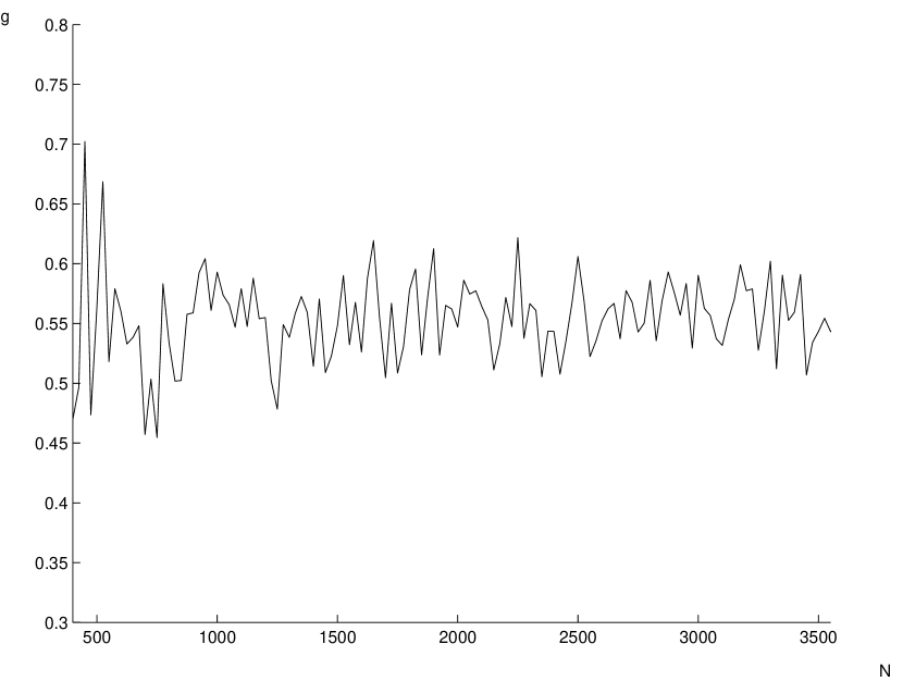
Figure 6: The stochastic graph, which shows $g(N)$ from Eq (52) as a function of $N$, is drawn for exactly the same conditions as those of Figure 5 except that the values of $\frac{n_{o_{j}}}{n}$ and $\frac{n_{i_{j}}}{n}$ are randomly chosen. Note that in contrast to Figure 5 some of these experiments may be identical due to the random conditions under which they are performed. Thus, the results do not show any clear-cut consistent value for the entropy differences.

We note that the same results may be obtained by using other methods and terminology. Thus, it is shown [19] that the “localization” (in the sense of smaller dispersion) for the state $|\phi\!>$ is greater the smaller is the entropy which results when the rate of “effective interaction with the environment” [19] increases. Localization is another name for what we call here “realizing or preserving a specific state” and the interaction with the environment is equivalent to performing experiment [20, 21, 22], so that as the rate of performing experiment grows the more realized and localized is the state one begins with or the path of states along which one proceeds.

Concluding Remarks

We have studied the influence of obsevation, and especially the large number of them, upon the obtained results. This has been shown for both quantum and classical systems. For the quantum part in Sections 2-3 we have made use of the Feynman path integral [8] and the Everett’s relative state [9, 10] methods. For the classical part in Section 4 we use entropy considerations [11] for discussing the four-piston cylinder [12]. Using these analytical methods we show that for producing the obtained results all the involved systems and experiments should be related to each other in some kind of relationship which assumes different, and even contradictory, forms for different situations. Thus, for the static Zeno effect the relationship between the systems is their being initially prepared in the same initial state and for the dynamic Zeno and the classical cylinder this relationship is effected by initially preparing the systems in different states.

This is, especially, emphasized in a clearer way using entropy considerations in Section 4. The important factor that entails the collective entropy decrease is, as remarked, when all the memebers of the ensemble are related to each other as described in Section 4 (see Figure 5). Unrelated ensemble of observers, no matter how large it is, does not obtain the same required entropy decrease as seen clearly in Figure 6.

References

- [1] J. A. Wheeler and H. Zurek, eds, “Quantum theory and measurement”, Princeton University Press, Princeton, New Jersey (1983); A. Daneri, A. Loinger and G. M. Prosperi, Nucl. phys, 33, 297-319 (1962).
- [2] C. B. Chiu, E. C. G. Sudarshan and B. Misra, Phys. Rev D, 16, 520-529, (1977; B. Misra and E. C. Sudarshan, J. Math. Phys,18, 756, (1977); D. Giulini, E. Joos, C. Kiefer, J. Kusch, I. O. Stamatescu and H. D. Zeh, “decoherence and the appearance of a classical world in quantum theory”, Springer-Verlag, (1996); Saverio Pascazio and Mikio Namiki, Phys. Rev A 50, 6, 4582, (1994); W. M. Itano, D. J. Heinzen, J. J. Bollinger, and D. J. Wineland, Phys. Rev A 41, 2295-2300, (1990); A. Peres, Phys. Rev D 39, 10, 2943, (1989); A. Peres and Amiram Ron, Phys. Rev A 42, 9, 5720, (1990); M. Bixon, Chem. Phys, 70, 199-206, (1982).
- [3] Marcus Simonius, Phys. Rev. Lett, 40, 15, 980-983, (1978);
- [4] W. M. Itano, D. J. Heinzen, J. J. Bollinger, and D. J. Wineland, Phys. Rev A, 41, 2295-2300, (1990); A. G. Kofman and G. Kurizki, Phys. Rev A, 54, 3750-3753, (1996); G. Kurizki, A. G. Kofman and V. Yudson, Phys. Rev A, 53, R35, (1995); S. R. Wilkinson, C. F. Bharucha, M. C. Madison, P. R. Morrow, Q. Niu, B. Sundaram and M. G. Raisen, Nature, 387, 575-577, (1997).
- [5] Y. Aharonov and M. Vardi, Phys. Rev D, 21, 2235, (1980);
- [6] P. Facchi, A. G. Klein, S. Pascazio and L. Schulman, Phys. Lett A 257, 232-240, (1999).
- [7] D. Bar and L. P. Horwitz, Int. Jour. Theor. Phys, 40, (10), 1697 (2001); Shunlong Luo, Physica A, 317, 509-516 (2003).
- [8] Richard. P. Feynman, Rev. Mod. Phys,20, 2, 367 (1948); “Quantum Mechanics and path integrals”, Richard. P. Feynman and A. R. Hibbs, McGraw-Hill Book Company (1965); G. Roepstorff, “Path integral approach to quantum physics”, Springer (1994); L. S. Schulman, "Techniques and applications of path intergrations”, John Wiley (1981).
- [9] H. Everett. III, Rev. Mod. Phys, 29, 454 (1957).
- [10] N. Graham in “The many worlds interpretation of QM”, B. S. Dewitt and N. Graham, eds, Princeton, Princeton University Press, (1973).
- [11] “Statistical Physics”, by F. Reif, Berkeley Physics Course, Vol 5, McGraw-Hill (1965).
- [12] L. Szilard, in “Quantum theory and measurement”, J. A. Wheeler and W. H. Zurek, eds, Princeton University Press, Princeton, New Jersey, (1983) (originally published in Zeitschrift Fur Physik, 53, 840-856 (1926)).
- [13] D. Bar, Found. Phys, 30, 813-838 (2000).
- [14] D. Finkelstein, Trans. NY. Acad. Sci, 25, 621, (1963).
- [15] J. B. Hartle, Am. J. Phys, 36, 704 (1966).
- [16] L. Smolin in “Quantum theory of gravity”, S. Christensen, ed, Adam-Hilger (1984).
- [17] E. Merzbacher, Quantum Mechanics", Second edition, Wiley, New York (1961); ‘‘Quantum Mechanics”, Claude Cohen Tannoudji, Bernard Diu and Franck Laloe, Wiley (1977)
- [18] M. R. Spiegel, “Probability and Statistics”, Schaum, McGRaw-Hill (1975).
- [19] N. Gisin and I. C. Percival, J. Phys. A: Math. Gen, 26, 2233-2243 (1993).
- [20] R. A. Harris and L. Stodolsky, J. Chem. Phys, 74, 4, 2145 (1981); Mordechai Bixon, Chem. Phys, 70, 199-206 (1982);
- [21] E.B.Davies, Ann. Inst. Henri Poincare A 28, 91 (1978); E.B.Davies, Commun. Math. Phys 64, 191 (1979); “Chiral molecules-A superselection rule induced by the radiation field” by P.Pfeifer, dissertation ETH No.6551, Zurich (1980).
- [22] E. Joos and H. D. Zeh, Z. Phys. B-Condensed Matter, 59, 223-243 (1985).