Antonina N. Fedorova, Michael G. Zeitlin

IPME RAS, St. Petersburg, V.O. Bolshoj pr., 61, 199178, Russia

e-mail: zeitlin@math.ipme.ru

http://www.ipme.ru/zeitlin.html

http://www.ipme.nw.ru/zeitlin.html RMS/RATE DYNAMICS VIA LOCALIZED MODES Antonina N. Fedorova    Michael G. Zeitlin IPME    RAS    V.O. Bolshoj pr    61    199178    St. Petersburg    Russia e-mail: zeitlin@math.ipme.ru http://www.ipme.ru/zeitlin.html; http://www.ipme.nw.ru/zeitlin.html Abstract We consider some reduction from nonlinear Vlasov-Maxwell equation to rms/rate equations for second moments related quantities. Our analysis is based on variational-wavelet approach to rational (in dynamical variables) approximation. It allows to control contribution from each scale of underlying multiscales and represent solutions via multiscale exact nonlinear eigenmodes (waveletons) expansions. Our approach provides the possibility to work with well-localized bases in phase space and best convergence properties of the corresponding expansions without perturbations or/and linearization procedures. Abstract We consider some reduction from nonlinear Vlasov-Maxwell equation to rms/rate equations for second moments related quantities. Our analysis is based on variational-wavelet approach to rational (in dynamical variables) approximation. It allows to control contribution from each scale of underlying multiscales and represent solutions via multiscale exact nonlinear eigenmodes (waveletons) expansions. Our approach provides the possibility to work with well-localized bases in phase space and best convergence properties of the corresponding expansions without perturbations or/and linearization procedures. Presented at the Eighth European Particle Accelerator Conference

EPAC’02

Paris, France, June 3-7, 2002

1 INTRODUCTION

In this paper we consider the applications of a new numerical-analytical technique based on the methods of local nonlinear harmonic analysis or wavelet analysis to nonlinear rms/rate equations for averaged quantities related to some particular case of nonlinear Vlasov-Maxwell equations. Our starting point is a model and approach proposed by R. C. Davidson e.a. [1], [2]. According to [1] we consider electrostatic approximation for a thin beam. This approximation is a particular important case of the general reduction from statistical collective description based on Vlasov-Maxwell equations to a finite number of ordinary differential equations for the second moments related quantities (beam radius and emittance). In our case these reduced rms/rate equations also contain some disribution averaged quantities besides the second moments, e.g. self-field energy of the beam particles. Such model is very efficient for analysis of many problems related to periodic focusing accelerators, e.g. heavy ion fusion and tritium production. So, we are interested in the understanding of collective properties, nonlinear dynamics and transport processes of intense non-neutral beams propagating through a periodic focusing field. Our approach is based on the variational-wavelet approach from [3]-[16],[17] that allows to consider rational type of nonlinearities in rms/rate dynamical equations containing statistically averaged quantities also. The solution has the multiscale/multiresolution decomposition via nonlinear high-localized eigenmodes (waveletons), which corresponds to the full multiresolution expansion in all underlying internal hidden scales. We may move from coarse scales of resolution to the finest one to obtain more detailed information about our dynamical process. In this way we give contribution to our full solution from each scale of resolution or each time/space scale or from each nonlinear eigenmode. Starting from some electrostatic approximation of Vlasov-Maxwell system and rms/rate dynamical models in part 2 we consider the approach based on variational-wavelet formulation in part 3. We give explicit representation for all dynamical variables in the bases of compactly supported wavelets or nonlinear eigenmodes. Our solutions are parametrized by the solutions of a number of reduced standard algebraical problems. We present also numerical modelling based on our analytical approach.

2 RATE EQUATIONS

In thin-beam approximation with negligibly small spread in axial momentum for beam particles we have in Larmor frame the following electrostatic approximation for Vlasov-Maxwell equations:

$$\frac{\partial F}{\partial s}+x^{\prime}\frac{\partial F}{\partial x}+y^{\prime}\frac{\partial F}{\partial y}-\Big{(}k(s)x+\frac{\partial\psi}{\partial x}\Big{)}\frac{\partial F}{\partial x^{\prime}}$$ (1)

$$-\Big{(}k(s)y+\frac{\partial\psi}{\partial y}\Big{)}\frac{\partial F}{\partial y^{\prime}}=0$$

$$\Big{(}\frac{\partial^{2}}{\partial x^{2}}+\frac{\partial^{2}}{\partial y^{2}}\Big{)}\psi=-\frac{2\pi K}{N}\int\mathrm{d}x^{\prime}\mathrm{d}y^{\prime}F$$ (2)

where $\psi(x,y,s)$ is normalized electrostatic potential and $F(x,y,x^{\prime},y^{\prime},s)$ is distribution function in transverse phase space $(x,y,x^{\prime},y^{\prime},s)$ with normalization

$$N=\int\mathrm{d}x\mathrm{d}yn,\qquad n(x,y,s)=\int\mathrm{d}x^{\prime}\mathrm{d}y^{\prime}F$$ (3)

where $K$ is self-field perveance which measures self-field intensity [1]. Introducing self-field energy

$$E(s)=\frac{1}{4\pi K}\int\mathrm{d}x\mathrm{d}y|\partial^{2}\psi/\partial x^{2}+\partial^{2}\psi/\partial y^{2}|$$ (4)

we have obvious equations for root-mean-square beam radius $R(s)$

$$R(s)=<x^{2}+y^{2}>^{1/2}$$ (5)

and unnormalized beam emittance $\qquad\varepsilon^{2}(s)=$

$$4(<x^{\prime 2}+y^{\prime 2}><x^{2}+y^{2}>-<xx^{\prime}-yy^{\prime}>),$$ (6)

which appear after averaging second-moments quantities regarding distribution function $F$:

$$\frac{\mathrm{d}^{2}R(s)}{\mathrm{d}s^{2}}+\Big{(}k(s)R(s)-\frac{K(1+\Delta)}{2R^{2}(s)}\Big{)}R(s)=\frac{\varepsilon^{2}(s)}{4R^{3}(s)}$$ (7)

$$\frac{\mathrm{d}\varepsilon^{2}(s)}{\mathrm{d}s}+8R^{2}(s)\Big{(}\frac{\mathrm{d}R}{\mathrm{d}s}\frac{K(1+\Delta)}{2R(s)}-\frac{\mathrm{d}E(s)}{\mathrm{d}s}\Big{)}=0,$$ (8)

where the term $K(1+\Delta)/2$ may be fixed in some interesting cases, but generally we have it only as average

$$K(1+\Delta)/2=-<x\partial\psi/\partial x+y\partial\psi/\partial y>$$ (9)

regarding distribution $F$. Anyway, the rate equations (7), (8) represent reasoanable reductions for the second-moments related quantities from the full nonlinear Vlasov-Poisson system. For trivial distributions Davidson e.a. [1] found additional reductions. For KV distribution (step-function density) the second rate equation (8) is trivial, $\varepsilon(s)$=const and we have only one nontrivial rate equation for rms beam radius (7). The fixed-shape density profile ansatz for axisymmetric distributions in [1] also leads to similar situation: emittance conservation and the same envelope equation with two shifted constants only.

3 MULTISCALE REPRESENTATIONS

Accordingly to our approach [3]-[16], [17] which allows us to find exact solutions as for Vlasov-like systems (1)-(3) as for rms-like systems (7),(8) we need not to fix particular case of distribution function $F(x,y,x^{\prime},y^{\prime},s)$. Our consideration is based on the following multiscale $N$-mode anzatz:

$$F^{N}(x,y,x^{\prime},y^{\prime},s)=$$ (10)

$$\sum^{N}_{i_{1},\dots,i_{5}=1}a_{i_{1},\dots,i_{5}}\bigotimes^{5}_{k=1}A_{i_{k}}(x,y,x^{\prime},y^{\prime},s)$$

$$\psi^{N}(x,y,s)=\sum^{N}_{j_{1},j_{2},j_{3}=1}b_{j_{1},j_{2},j_{3}}\bigotimes^{3}_{k=1}B_{j_{k}}(x,y,s)$$ (11)

Formulae (10), (11) provide multiresolution representation for variational solutions of system (1)-(3) [3]-[16],[17]. Each high-localized mode/harmonics $A_{j}(s)$ corresponds to level $j$ of resolution from the whole underlying infinite scale of spaces: $\dots V_{-2}\subset V_{-1}\subset V_{0}\subset V_{1}\subset V_{2}\subset\dots,$ where the closed subspace $V_{j}(j\in{\bf Z})$ corresponds to level j of resolution, or to scale j. The construction of such tensor algebra based multiscales bases are considered in [17]. We’ll consider rate equations (7), (8) as the following operator equation. Let $L$, $P$, $Q$ be an arbitrary nonlinear (rational in dynamical variables) first-order matrix differential operators with matrix dimension d (d=4 in our case) corresponding to the system of equations (7)-(8), which act on some set of functions $\Psi\equiv\Psi(s)=\Big{(}\Psi^{1}(s),\dots,\Psi^{d}(s)\Big{)},\quad s\in\Omega\subset R$ from $L^{2}(\Omega)$: $Q(R,s)\Psi(s)=P(R,s)\Psi(s)$ or

$$L\Psi\equiv L(R,s)\Psi(s)=0$$ (12)

where $R\equiv R(s,\partial/\partial s,\Psi)$. Let us consider now the N mode approximation for solution as the following expansion in some high-localized wavelet-like basis:

$$\Psi^{N}(s)=\sum^{N}_{r=1}a^{N}_{r}\phi_{r}(s)$$ (13)

We shall determine the coefficients of expansion from the following variational conditions (different related variational approaches are considered in [3]-[16]):

$$L^{N}_{k}\equiv\int(L\Psi^{N})\phi_{k}(s)\mathrm{d}s=0$$ (14)

We have exactly $dN$ algebraical equations for $dN$ unknowns $a_{r}$. So, variational approach reduced the initial problem (7), (8) to the problem of solution of functional equations at the first stage and some algebraical problems at the second stage. As a result we have the following reduced algebraical system of equations (RSAE) on the set of unknown coefficients $a_{i}^{N}$ of expansion (14):

$$H(Q_{ij},a_{i}^{N},\alpha_{I})=M(P_{ij},a_{i}^{N},\beta_{J}),$$ (15)

where operators $H$ and $M$ are algebraization of RHS and LHS of initial problem (12). $Q_{ij}$ ($P_{ij}$) are the coefficients of LHS (RHS) of the initial system of differential equations (7), (8) and as consequence are coefficients of RSAE. $I=(i_{1},...,i_{q+2})$, $J=(j_{1},...,j_{p+1})$ are multiindexes, by which are labelled $\alpha_{I}$ and $\beta_{I}$, the other coefficients of RSAE (15):

$$\beta_{J}=\{\beta_{j_{1}...j_{p+1}}\}=\int\prod_{1\leq j_{k}\leq p+1}\phi_{j_{k}},$$ (16)

where $p$ is the degree of polynomial operator $P$ (12)

$$\alpha_{I}=\{\alpha_{i_{1}}...\alpha_{i_{q+2}}\}=\sum_{i_{1},...,i_{q+2}}\int\phi_{i_{1}}...\dot{\phi_{i_{s}}}...\phi_{i_{q+2}},$$ (17)

where $q$ is the degree of polynomial operator $Q$ (12), $i_{\ell}=(1,...,q+2)$, $\dot{\phi_{i_{s}}}=\mathrm{d}\phi_{i_{s}}/\mathrm{d}s$. According to [3]-[16] we may extend our approach to the case when we have additional constraints as (3) on the set of our dynamical variables $\Psi$={$R$, $\varepsilon\}$ and additional averaged terms (4), (9) also. In this case by using the method of Lagrangian multipliers we again may apply the same approach but for the extended set of variables. As a result we receive the expanded system of algebraical equations analogous to the system (15). Then, after reduction we again can extract from its solution the coefficients of expansion (13). It should be noted that if we consider only truncated expansion (13) with N terms then we have the system of $N\times d$ algebraical equations with the degree $\ell=max\{p,q\}$ and the degree of this algebraical system coincides with the degree of the initial system. So, after all we have the solution of the initial nonlinear (rational) problem in the form

$$R^{N}(s) = R(0)+\sum_{k=1}^{N}a_{k}^{N}\phi_{k}(s)$$ (18)

$$\varepsilon^{N}(s) = \varepsilon(0)+\sum_{k=1}^{N}b_{k}^{N}\phi_{k}(s)$$ (19)

where coefficients $a_{k}^{N}$, $b_{k}^{N}$ are the roots of the corresponding reduced algebraical (polynomial) problem RSAE (15). Consequently, we have a parametrization of the solution of the initial problem by solution of reduced algebraical problem (15). The problem of computations of coefficients $\alpha_{I}$ (17), $\beta_{J}$ (16) of reduced algebraical system may be explicitly solved in wavelet approach. The obtained solutions are given in the form (18, (19), where $\phi_{k}(s)$ are proper wavelet bases functions (e.g., periodic or boundary). It should be noted that such representations give the best possible localization properties in the corresponding (phase)space/time coordinates. In contrast with different approaches formulae (18), (19) do not use perturbation technique or linearization procedures and represent dynamics via generalized nonlinear localized eigenmodes expansion.

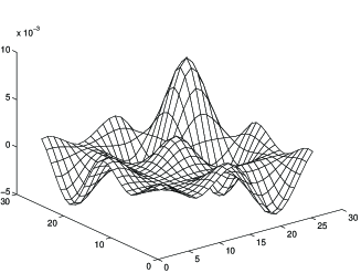
Figure 1: Waveleton-like distribution.

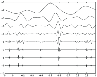
Figure 2: Multiscale decomposition.

Our N mode construction (18), (19) gives the following general multiscale representation:

$$R(s) = R_{N}^{slow}(s)+\sum_{i\geq N}R^{i}(\omega_{i}s),\quad\omega_{i}\sim 2^{i}$$

$$\varepsilon(s) = \varepsilon_{N}^{slow}(s)+\sum_{j\geq N}\varepsilon^{j}(\omega_{j}s),\quad\omega_{j}\sim 2^{j}$$

where $R^{i}(s),\varepsilon^{j}(s)$ are represented by some family of (nonlinear) eigenmodes and gives the full multiresolution/multiscale representation in the high-localized wavelet bases. The corresponding decomposition is presented on Fig. 2 and two-dimensional localized mode (waveleton) contribution to distribution function is presented on Fig.1. As a result we can construct different (stable) patterns from high-localized (coherent) structures in spatially-extended stochastic systems with complex collective behaviour.

References

- [1] R.C. Davidson, e.a., Phys. Plasmas, 5, 279, 1998
- [2] The Physics of High Brightness Beams, Ed.J. Rosenzweig & L. Serafini, World Scientific, 2000.
- [3] A.N. Fedorova and M.G. Zeitlin, Math. and Comp. in Simulation, 46, 527, 1998.
- [4] A.N. Fedorova and M.G. Zeitlin, New Applications of Nonlinear and Chaotic Dynamics in Mechanics, 31, 101 Kluwer, 1998.
- [5] A.N. Fedorova and M.G. Zeitlin, CP405, 87, American Institute of Physics, 1997. Los Alamos preprint, physics/9710035.
- [6] A.N. Fedorova, M.G. Zeitlin and Z. Parsa, Proc. PAC97 2, 1502, 1505, 1508, APS/IEEE, 1998.
- [7] A.N. Fedorova, M.G. Zeitlin and Z. Parsa, Proc. EPAC98, 930, 933, Institute of Physics, 1998.
- [8] A.N. Fedorova, M.G. Zeitlin and Z. Parsa, CP468, 48, American Institute of Physics, 1999. Los Alamos preprint, physics/990262.
- [9] A.N. Fedorova, M.G. Zeitlin and Z. Parsa, CP468, 69, American Institute of Physics, 1999. Los Alamos preprint, physics/990263.
- [10] A.N. Fedorova and M.G. Zeitlin, Proc. PAC99, 1614, 1617, 1620, 2900, 2903, 2906, 2909, 2912, APS/IEEE, New York, 1999. Los Alamos preprints: physics/9904039, 9904040, 9904041, 9904042, 9904043, 9904045, 9904046, 9904047.
- [11] A.N. Fedorova and M.G. Zeitlin, The Physics of High Brightness Beams, 235, World Scientific, 2000. Los Alamos preprint: physics/0003095.
- [12] A.N. Fedorova and M.G. Zeitlin, Proc. EPAC00, 415, 872, 1101, 1190, 1339, 2325, Austrian Acad.Sci.,2000. Los Alamos preprints: physics/0008045, 0008046, 0008047, 0008048, 0008049, 0008050.
- [13] A.N. Fedorova, M.G. Zeitlin, Proc. 20 International Linac Conf., 300, 303, SLAC, Stanford, 2000. Los Alamos preprints: physics/0008043, 0008200.
- [14] A.N. Fedorova, M.G. Zeitlin, Los Alamos preprints: physics/0101006, 0101007 and World Scientific, in press.
- [15] A.N. Fedorova, M.G. Zeitlin, Proc. PAC2001, Chicago, 790-1792, 1805-1807, 1808-1810, 1811-1813, 1814-1816, 2982-2984, 3006-3008, IEEE, 2002 or arXiv preprints: physics/0106022, 0106010, 0106009, 0106008, 0106007, 0106006, 0106005.
- [16] A.N. Fedorova, M.G. Zeitlin, Proc. in Applied Mathematics and Mechanics, 1, Issue 1, pp. 399-400, 432-433, Wiley-VCH, 2002.
- [17] A.N. Fedorova, M.G. Zeitlin, this Proc.