SPECTRUM OF BEAM-BEAM INTERACTIONS Antonina N. Fedorova, Michael G. Zeitlin

IPME RAS, St. Petersburg, V.O. Bolshoj pr., 61, 199178, Russia

e-mail: zeitlin@math.ipme.ru

http://www.ipme.ru/zeitlin.html

http://www.ipme.nw.ru/zeitlin.html NONLINEAR LOCALIZED COHERENT SPECTRUM OF BEAM-BEAM INTERACTIONS Antonina N. Fedorova    Michael G. Zeitlin IPME    RAS    St. Petersburg    V.O. Bolshoj pr    61    199178    Russia e-mail: zeitlin@math.ipme.ruhttp://www.ipme.ru/zeitlin.html; http://www.ipme.nw.ru/zeitlin.html Abstract We consider modeling for strong-strong beam-beam interactions beyond preceding linearized/perturbative methods such as soft gaussian approximation or FMM (HFMM) etc. In our approach discrete coherent modes, discovered before, and possible incoherent oscillations appear as a result of multiresolution/multiscale fast convergent decomposition in the bases of high-localized exact nonlinear modes represented by wavelets or wavelet packets functions. The constructed solutions represent the full multiscale spectrum in all internal hidden scales from slow to fast oscillating eigenmodes. Underlying variational method provides algebraical control of the spectrum. Abstract We consider modeling for strong-strong beam-beam interactions beyond preceding linearized/perturbative methods such as soft gaussian approximation or FMM (HFMM) etc. In our approach discrete coherent modes, discovered before, and possible incoherent oscillations appear as a result of multiresolution/multiscale fast convergent decomposition in the bases of high-localized exact nonlinear modes represented by wavelets or wavelet packets functions. The constructed solutions represent the full multiscale spectrum in all internal hidden scales from slow to fast oscillating eigenmodes. Underlying variational method provides algebraical control of the spectrum. Presented at the Eighth European Particle Accelerator Conference

EPAC’02

Paris, France, June 3-7, 2002

1 INTRODUCTION

We consider the first steps of analysis of beam-beam interactions in some collective model approach. It is well-known that neither direct PIC modeling nor soft-gaussian approximation provide reasonable resolution of computing time/noise problems and understanding of underlying complex nonlinear dynamics [1], [2]. Recent analysis, based as on numerical simulation as on modeling, demonstrates that presence of coherent modes inside the spectrum leads to oscillations and growth of beam transverse size and deformations of beam shape. This leads to strong limitations for operation of LHC. Additional problems appear as a result of continuum spectrum of incoherent oscillations in each beam. The strong-strong collisions of two beams also lead to variation of transverse size. According to [2] it is reasonable to find nonperturbative solutions at least in the important particular cases. Our approach based on wavelet analysis technique is in some sense the direct generalization of Fast Multipole Method (FMM) and related approaches (HFMM). After set-up based on Vlasov-like model (according [2]) in part 2, we consider variational-wavelet approach [3]-[17] in framework of powerful technique based on Fast Wavelet Transform (FWT) operator representations [18] in section 3. As a result we have multiresolution/multiscale fast convergent decomposition in the bases of high-localized exact nonlinear eigenmodes represented by wavelets or wavelet packets functions. The constructed solutions represent the full multiscale spectrum in all internal hidden scales from slow to fast oscillating eigenmodes. Underlying variational method provides algebraical control of the spectrum.

2 VLASOV MODEL FOR BEAM-BEAM INTERACTIONS

Vlasov-like equations describing evolution of the phase space distributions $\psi^{j}=\psi^{j}(x,p_{x},\theta)$ ($j=1,2$) for each beam are [2]:

$$\frac{\partial\psi^{j}}{\partial\theta}=-q_{x}p_{x}\frac{\partial\psi^{j}}{\partial x}+$$ (1)

$$\Big{(}q_{x}x+\delta_{p}(\theta)4\pi\xi_{x}p.v.\int^{\infty}_{-\infty}\frac{\rho^{*}(x^{\prime},\theta)}{x-x^{\prime}}\mathrm{d}x^{\prime}\Big{)}\frac{\partial\psi^{j}}{\partial p_{x}}$$

where

$$\rho^{*}(x,\theta)=\int^{\infty}_{-\infty}\psi^{*}(x,p_{x},\theta)\mathrm{d}p_{x}$$ (2)

and $\psi^{*}$ is the density of the opposite beam, $q_{x}$ is unperturbed fractional tune, $\xi_{x}$ is horizontal beam-beam parameter, $N$ is a number of particles, $x$, $p_{x}$ are normalized variables. This model describes horizontal oscillations of flat beams with one bunch per beam, one interaction point, equal energy, population and optics for both beams.

3 FWT BASED VARIATIONAL APPROACH

One of the key points of wavelet approach demonstrates that for a large class of operators wavelets are good approximation for true eigenvectors and the corresponding matrices are almost diagonal. FWT [18] gives the maximum sparse form of operators under consideration (1). It is true also in case of our Vlasov-like system of equations (1). We have both differential and integral operators inside. So, let us denote our (integral/differential) operator from equations (1) as $T$ ($L^{2}(R^{n})\rightarrow L^{2}(R^{n})$) and its kernel as $K$. We have the following representation:

$$<Tf,g>=\int\int K(x,y)f(y)g(x)\mathrm{d}x\mathrm{d}y$$ (3)

In case when $f$ and $g$ are wavelets $\varphi_{j,k}=2^{j/2}\varphi(2^{j}x-k)$ (3) provides the standard representation for operator $T$. Let us consider multiresolution representation $\dots\subset V_{2}\subset V_{1}\subset V_{0}\subset V_{-1}\subset V_{-2}\dots$. The basis in each $V_{j}$ is $\varphi_{j,k}(x)$, where indices $\ k,j$ represent translations and scaling respectively. Let $P_{j}:L^{2}(R^{n})\rightarrow V_{j}$ $(j\in Z)$ be projection operators on the subspace $V_{j}$ corresponding to level $j$ of resolution: $(P_{j}f)(x)=\sum_{k}<f,\varphi_{j,k}>\varphi_{j,k}(x).$ Let $Q_{j}=P_{j-1}-P_{j}$ be the projection operator on the subspace $W_{j}$ ($V_{j-1}=V_{j}\oplus W_{j}$) then we have the following ”microscopic or telescopic” representation of operator T which takes into account contributions from each level of resolution from different scales starting with the coarsest and ending to the finest scales [18]:

$$T=\sum_{j\in Z}(Q_{j}TQ_{j}+Q_{j}TP_{j}+P_{j}TQ_{j}).$$ (4)

We remember that this is a result of presence of affine group inside this construction. The non-standard form of operator representation [18] is a representation of operator T as a chain of triples $T=\{A_{j},B_{j},\Gamma_{j}\}_{j\in Z}$, acting on the subspaces $V_{j}$ and $W_{j}$: $A_{j}:W_{j}\rightarrow W_{j},B_{j}:V_{j}\rightarrow W_{j},\Gamma_{j}:W_{j}\rightarrow V_{j},$ where operators $\{A_{j},B_{j},\Gamma_{j}\}_{j\in Z}$ are defined as $A_{j}=Q_{j}TQ_{j},\quad B_{j}=Q_{j}TP_{j},\quad\Gamma_{j}=P_{j}TQ_{j}.$ The operator $T$ admits a recursive definition via

$$T_{j}=\left(\begin{array}[]{cc}A_{j+1}&B_{j+1}\\ \Gamma_{j+1}&T_{j+1}\end{array}\right),$$ (7)

where $T_{j}=P_{j}TP_{j}$ and $T_{j}$ acts on $V_{j}:V_{j}\rightarrow V_{j}$. It should be noted that operator $A_{j}$ describes interaction on the scale $j$ independently from other scales, operators $B_{j},\Gamma_{j}$ describe interaction between the scale j and all coarser scales, the operator $T_{j}$ is an ”averaged” version of $T_{j-1}$. We may compute such non-standard representations for different operators (including Calderon-Zygmund or pseudodifferential). As in case of differential operator as in other cases we need only to solve the system of linear algebraical equations. The action of integral operator in equations (1) we may consider as a Hilbert transform

$$(H\rho^{*})(x)=\frac{1}{\pi}p.v.\int^{\infty}_{-\infty}\frac{\rho^{*}(x^{\prime},\theta)}{x^{\prime}-x}\mathrm{d}x^{\prime}$$ (8)

The representation of $H$ on $V_{0}$ is defined by the coefficients

$$r_{\ell}=\int\varphi(x-\ell)(H\varphi)(x)\mathrm{d}x,\quad\ell\in Z.$$ (9)

which according to $FWT$ technique define also all other coefficients of the nonstandard representation. So we have $H=\{A_{j},B_{j},\Gamma_{j}\}_{j\in Z}$ with the corresponding matrix elements $a_{i-\ell},b_{i-\ell},c_{i-\ell}$ which can be computed from coefficients $r_{\ell}$ only:

$$a_{i} = \sum^{L-1}_{k,k^{\prime}=0}g_{k}g_{k^{\prime}}r_{2i+k-k^{\prime}}$$

$$b_{i} = \sum^{L-1}_{k,k^{\prime}=0}g_{k}h_{k^{\prime}}r_{2i+k-k^{\prime}}$$ (10)

$$c_{i} = \sum^{L-1}_{k,k^{\prime}=0}h_{k}g_{k^{\prime}}r_{2i+k-k^{\prime}}$$

The coefficients $r_{\ell}$ (7) can be obtained from

$$r_{\ell}=r_{2\ell}+\sum^{L/2}_{k=1}d_{2k-1}(r_{2\ell-2k+1}+r_{2\ell+2k-1})$$ (11)

where $d_{n}$ are the so called autocorrelation coefficients of the corresponding quadratic mirror filter $\quad\{h_{k}\}^{L-1}_{k=0}$: $\qquad d_{n}=2\sum^{L-1-n}_{i=0}h_{i}h_{i+n}$, $n=1,\dots,L-1,$ $d_{2k}=0$, $k=1,\dots,L/2-1$, $g_{k}=(-1)^{k}h_{L-k-1}$, $k=0,\dots,L-1$, which parametrizes the basic refinement equation $\varphi(x)=\sqrt{2}\sum^{L-1}_{k=0}h_{k}\varphi(2x-k).$ This equation really generates all wavelet zoo. It is useful to add to the system (9) the following asymptotic condition $r_{\ell}=-1/\pi\ell+O(\ell^{-2M})$, which simplifies the solution procedure. Then finally we have the following action of operator $T_{j}$ on sufficiently smooth function $f$:

$$(T_{j}f)(x)=\sum_{k\in Z}\left(2^{-j}\sum_{\ell}r_{\ell}f_{j,k-\ell}\right)\varphi_{j,k}(x),$$ (12)

in the wavelet basis $\varphi_{j,k}(x)=2^{-j/2}\varphi(2^{-j}x-k)$ where

$$f_{j,k-1}=2^{-j/2}\int f(x)\varphi(2^{-j}x-k+\ell)\mathrm{d}x$$ (13)

are wavelet coefficients. So, we have simple linear parametrization of matrix representation of our operator (6) in wavelet bases and of the action of this operator on arbitrary vector in proper functional space. The similar approach can be applied to other operators in (1). Then we may apply our variational approach from [3]-[17]. Let L be an arbitrary (non) linear (differential/integral) operator corresponds to the system (1) with matrix dimension $d$, which acts on some set of functions $\quad\Psi\equiv\Psi(\theta,x,p_{x})=$ $\Big{(}\Psi^{1}(\theta,x,p_{x}),\dots,$ $\Psi^{d}(\theta,x,p_{x})\Big{)}$, $\quad\theta,x,p_{x}\in\Omega\subset{\bf R}^{3}$, $L\Psi\equiv L(Q,\theta,x,p_{x})\Psi(\theta,x,p_{x})=0,$ where $Q\equiv Q_{d_{1},d_{2},d_{3}}(\theta,x,p_{x},\partial/\partial\theta,\partial/\partial x,\partial/\partial p_{x},\int\mathrm{d}x\mathrm{d}p_{x})$. Let us consider now the N mode approximation for solution as the following ansatz (in the same way we may consider different ansatzes) [17]:

$$\Psi^{N}(\theta,x,p_{x})=\sum^{N}_{r,s,k=1}a_{rsk}A_{r}\otimes B_{s}\otimes C_{k}(\theta,x,p_{x})$$ (14)

We shall determine the coefficients of expansion from the following conditions (different related variational approaches are considered in [3]-[16]): ℓ^N_kℓm≡∫(LΨ^N)A_k(θ)B_ℓ(x)C_m(p_x)dθdxdp_x=0 So, we have exactly $dN^{3}$ algebraical equations for $dN^{3}$ unknowns $a_{rsk}$. The solution is parametrized by solutions of two set of reduced algebraical problems, one is linear or nonlinear (depends on the structure of operator L) and the rest are some linear problems related to computation of coefficients of algebraic equations. These coefficients can be found by some wavelet methods by using compactly supported wavelet basis functions for expansions (12). We may consider also different types of wavelets including general wavelet packets. The constructed solution has the following multiscale/multiresolution decomposition via nonlinear high-localized eigenmodes

$$\psi(\theta,x,p_{x})=\sum_{(i,j,k)\in Z^{3}}a_{ijk}A^{i}(\theta)B^{j}(x)C^{k}(p_{x}),$$ (15)

$$A^{i}(\theta)=A_{N}^{i,slow}(\theta)+\sum_{r\geq N}A^{i}_{r}(\omega_{r}\theta),\ \omega_{r}\sim 2^{r}$$

$$B^{j}(x)=B_{M}^{j,slow}(x)+\sum_{l\geq M}B^{j}_{l}(k^{1}_{l}x),\ k^{1}_{l}\sim 2^{l}$$

$$C^{s}(p_{x})=C_{L}^{s,slow}(p_{x})+\sum_{m\geq L}C^{s}_{m}(k^{2}_{m}p_{x}),\ k^{2}_{m}\sim 2^{m}$$

which corresponds to the full multiresolution expansion in all underlying time/space scales.

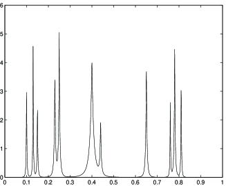
Figure 1: Region of nonlinear resonances.

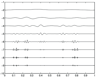
Figure 2: Eigenmodes decomposition.

Formula (15) gives us expansion into the slow part $f_{N,M,L}^{slow}$ and fast oscillating parts for arbitrary N, M, L. So, we may move from coarse scales of resolution to the finest one to obtain more detailed information about our dynamical process. The first terms in the RHS of formulae (13) correspond on the global level of function space decomposition to resolution space and the second ones to detail space. The using of wavelet basis with high-localized properties provides fast convergence of constructed decomposition (13). In contrast with different approaches, formulae (13) does not use perturbation technique or linearization procedures and represents dynamics via generalized nonlinear localized eigenmodes expansion. Numerical calculations are based on compactly supported wavelets and related wavelet families. Figures 1,2 demonstrate resonances region and corresponding nonlinear coherent eigenmodes decomposition according to representation (13).

References

- [1] K.Yokoya, Phys.Rev. ST AB, 3, 124401, 2000, M.P. Zorzano, F. Zimmerman, Phys.Rev. ST AB, 3, 044401, 2000
- [2] M.P. Zorzano, LHC Report 440, CERN, 2000
- [3] A.N. Fedorova and M.G. Zeitlin, Math. and Comp. in Simulation, 46, 527, 1998.
- [4] A.N. Fedorova and M.G. Zeitlin, New Applications of Nonlinear and Chaotic Dynamics in Mechanics, 31, 101 Kluwer, 1998.
- [5] A.N. Fedorova and M.G. Zeitlin, CP405, 87, American Institute of Physics, 1997. Los Alamos preprint, physics/9710035.
- [6] A.N. Fedorova, M.G. Zeitlin and Z. Parsa, Proc. PAC97 2, 1502, 1505, 1508, APS/IEEE, 1998.
- [7] A.N. Fedorova, M.G. Zeitlin and Z. Parsa, Proc. EPAC98, 930, 933, Institute of Physics, 1998.
- [8] A.N. Fedorova, M.G. Zeitlin and Z. Parsa, CP468, 48, American Institute of Physics, 1999. Los Alamos preprint, physics/990262.
- [9] A.N. Fedorova, M.G. Zeitlin and Z. Parsa, CP468, 69, American Institute of Physics, 1999. Los Alamos preprint, physics/990263.
- [10] A.N. Fedorova and M.G. Zeitlin, Proc. PAC99, 1614, 1617, 1620, 2900, 2903, 2906, 2909, 2912, APS/IEEE, New York, 1999. Los Alamos preprints: physics/9904039, 9904040, 9904041, 9904042, 9904043, 9904045, 9904046, 9904047.
- [11] A.N. Fedorova and M.G. Zeitlin, The Physics of High Brightness Beams, 235, World Scientific, 2000. Los Alamos preprint: physics/0003095.
- [12] A.N. Fedorova and M.G. Zeitlin, Proc. EPAC00, 415, 872, 1101, 1190, 1339, 2325, Austrian Acad.Sci.,2000. Los Alamos preprints: physics/0008045, 0008046, 0008047, 0008048, 0008049, 0008050.
- [13] A.N. Fedorova, M.G. Zeitlin, Proc. 20 International Linac Conf., 300, 303, SLAC, Stanford, 2000. Los Alamos preprints: physics/0008043, 0008200.
- [14] A.N. Fedorova, M.G. Zeitlin, Los Alamos preprints: physics/0101006, 0101007 and World Scientific, in press.
- [15] A.N. Fedorova, M.G. Zeitlin, Proc. PAC2001, Chicago, 790-1792, 1805-1807, 1808-1810, 1811-1813, 1814-1816, 2982-2984, 3006-3008, IEEE, 2002 or arXiv preprints: physics/0106022, 0106010, 0106009, 0106008, 0106007, 0106006, 0106005.
- [16] A.N. Fedorova, M.G. Zeitlin, Proc. in Applied Mathematics and Mechanics, 1, Issue 1, pp. 399-400, 432-433, Wiley-VCH, 2002.
- [17] A.N. Fedorova, M.G. Zeitlin, this Proc.
- [18] G. Beylkin, R. Coifman, V. Rokhlin, CPAM,44, 141, 1991