VLASOV-POISSON EQUATIONS Antonina N. Fedorova, Michael G. Zeitlin

IPME RAS, St. Petersburg, V.O. Bolshoj pr., 61, 199178, Russia

e-mail: zeitlin@math.ipme.ru

http://www.ipme.ru/zeitlin.html

http://www.ipme.nw.ru/zeitlin.html MULTISCALE DECOMPOSITION FOR VLASOV-POISSON EQUATIONS Antonina N. Fedorova    Michael G. Zeitlin IPME    RAS    V.O. Bolshoj pr    61    199178    St. Petersburg    Russia e-mail: zeitlin@math.ipme.ru http://www.ipme.ru/zeitlin.html; http://www.ipme.nw.ru/zeitlin.html Abstract We consider the applications of a numerical-analytical approach based on multiscale variational wavelet technique to the systems with collective type behaviour described by some forms of Vlasov-Poisson/Maxwell equations. We calculate the exact fast convergent representations for solutions in high-localized wavelet-like bases functions, which correspond to underlying hidden (coherent) nonlinear eigenmodes. This helps to control stability/unstability scenario of evolution in parameter space on pure algebraical level. Abstract We consider the applications of a numerical-analytical approach based on multiscale variational wavelet technique to the systems with collective type behaviour described by some forms of Vlasov-Poisson/Maxwell equations. We calculate the exact fast convergent representations for solutions in high-localized wavelet-like bases functions, which correspond to underlying hidden (coherent) nonlinear eigenmodes. This helps to control stability/unstability scenario of evolution in parameter space on pure algebraical level. Presented at the Eighth European Particle Accelerator Conference

EPAC’02

Paris, France, June 3-7, 2002

1 INTRODUCTION

In this paper we consider the applications of numerical-analytical approach based on multiscale variational wavelet technique to the systems with collective type behaviour described by some forms of Vlasov-Poisson/Maxwell equations [1], [2]. Such approach may be useful in all models in which it is possible and reasonable to reduce all complicated problems related with statistical distributions to the problems described by the systems of nonlinear ordinary/partial differential/integral equations with or without some (functional) constraints. In periodic accelerators and transport systems at the high beam currents and charge densities the effects of the intense self-fields, which are produced by the beam space charge and currents, determinine (possible) equilibrium states, stability and transport properties according to underlying nonlinear dynamics [2]. The dynamics of such space-charge dominated high brightness beam systems can provide the understanding of the instability phenomena such as emittance growth, mismatch, halo formation related to the complicated behaviour of underlying hidden nonlinear modes outside of perturbative tori-like KAM regions. Our analysis is based on the variational-wavelet approach from [3]-[17], which allows us to consider polynomial and rational type of nonlinearities. In some sense our approach is direct generaliztion of traditional nonlinear $\delta F$ approach in which weighted Klimontovich representation

$$\delta f_{j}=a_{j}\sum^{N_{j}}_{i=1}w_{ji}\delta(x-x_{ji})\delta(p-p_{ji})$$ (1)

or self-similar decompostion [2] like

$$\delta n_{j}=b_{j}\sum^{N_{j}}_{i=1}w_{ji}s(x-x_{ji}),$$ (2)

where $s(x-x_{ji})$ is a shape function of distributing particles on the grids in configuration space, are replaced by powerful technique from local nonlinear harmonic analysis, based on underlying symmetries of functional space such as affine or more general. The solution has the multiscale/multiresolution decomposition via nonlinear high-localized eigenmodes, which corresponds to the full multiresolution expansion in all underlying time/phase space scales. Starting from Vlasov-Poisson equations in part 2, we consider the approach based on multiscale variational-wavelet formulation in part 3. We give the explicit representation for all dynamical variables in the base of compactly supported wavelets or nonlinear eigenmodes. Our solutions are parametrized by solutions of a number of reduced algebraical problems one from which is nonlinear with the same degree of nonlinearity as initial problem and the others are the linear problems which correspond to the particular method of calculations inside concrete wavelet scheme. Because our approach started from variational formulation we can control evolution of instability on the pure algebraical level of reduced algebraical system of equations. This helps to control stability/unstability scenario of evolution in parameter space on pure algebraical level. In all these models numerical modeling demonstrates the appearance of coherent high-localized structures and as a result the stable patterns formation or unstable chaotic behaviour.

2 VLASOV-POISSON EQUATIONS

Analysis based on the non-linear Vlasov equations leads to more clear understanding of collective effects and nonlinear beam dynamics of high intensity beam propagation in periodic-focusing and uniform-focusing transport systems. We consider the following form of equations (ref. [1] for setup and designation):

$$\Big{\{}\frac{\partial}{\partial s}+p_{x}\frac{\partial}{\partial x}+p_{y}\frac{\partial}{\partial y}-\Big{[}k_{x}(s)x+\frac{\partial\psi}{\partial x}\Big{]}\frac{\partial}{\partial p_{x}}-$$

$$\Big{[}k_{y}(s)y+\frac{\partial\psi}{\partial y}\Big{]}\frac{\partial}{\partial p_{y}}\Big{\}}f_{b}(x,y,p_{x},p_{y},s)=0,$$ (3)

$$\Big{(}\frac{\partial^{2}}{\partial x^{2}}+\frac{\partial^{2}}{\partial y^{2}}\Big{)}\psi=-\frac{2\pi K_{b}}{N_{b}}\int\mathrm{d}p_{x}\mathrm{d}p_{y}f_{b},$$ (4)

$$\int\mathrm{d}x\mathrm{d}y\mathrm{d}p_{x}\mathrm{d}p_{y}f_{b}=N_{b}$$ (5)

The corresponding Hamiltonian for transverse single-particle motion is given by

$$H(x,y,p_{x},p_{y},s)=\frac{1}{2}(p_{x}^{2}+p_{y}^{2})+\frac{1}{2}[k_{x}(s)x^{2}$$ (6)

$$+k_{y}(s)y^{2}]+H_{1}(x,y,p_{x},p_{y},s)+\psi(x,y,s),$$

where $H_{1}$ is nonlinear (polynomial/rational) part of the full Hamiltonian and corresponding characteristic equations are:

$$\frac{\mathrm{d}^{2}x}{\mathrm{d}s^{2}}+k_{x}(s)x+\frac{\partial}{\partial x}\psi(x,y,s) = 0$$ (7)

$$\frac{\mathrm{d}^{2}y}{\mathrm{d}s^{2}}+k_{y}(s)y+\frac{\partial}{\partial y}\psi(x,y,s) = 0$$ (8)

3 MULTISCALE REPRESENTATIONS

We obtain our multiscale/multiresolution representations for solutions of equations (3)-(8) via variational-wavelet approach. We decompose the solutions as

$$f_{b}(s,x,y,p_{x},p_{y})=\sum^{\infty}_{i=i_{c}}\oplus\delta^{i}f(s,x,y,p_{x},p_{y})$$ (9)

$$\psi(s,x,y)=\sum^{\infty}_{j=j_{c}}\oplus\delta^{j}\psi(s,x,y)$$ (10)

$$x(s)=\sum^{\infty}_{k=k_{c}}\oplus\delta^{k}x(s),\quad y(s)=\sum^{\infty}_{\ell=\ell_{c}}\oplus\delta^{\ell}y(s)$$ (11)

where set $(i_{c},j_{c},k_{c},\ell_{c})$ corresponds to the coarsest level of resolution $c$ in the full multiresolution decomposition

$$V_{c}\subset V_{c+1}\subset V_{c+2}\subset\dots$$ (12)

Introducing detail space $W_{j}$ as the orthonormal complement of $V_{j}$ with respect to $V_{j+1}:V_{j+1}=V_{j}\bigoplus W_{j}$, we have for $f$, $\psi$, $x$, $y$ $\subset L^{2}({\bf R})$ from (9)-(11):

$$L^{2}({\bf R})=\overline{V_{c}\displaystyle\bigoplus^{\infty}_{j=c}W_{j}},$$ (13)

In some sense (9)-(11) is some generalization of the old $\delta F$ approach [1], [2]. Let $L$ be an arbitrary (non) linear differential/integral operator with matrix dimension $d$, which acts on some set of functions $\Psi\equiv\Psi(s,x)=\Big{(}\Psi^{1}(s,x),\dots,\Psi^{d}(s,x)\Big{)}$, $s,x\in\Omega\subset{\bf R}^{n+1}$ from $L^{2}(\Omega)$:

$$L\Psi\equiv L(R(s,x),s,x)\Psi(s,x)=0,$$ (14)

($x$ are the generalized space coordinates or phase space coordinates, $s$ is “time” coordinate). After some anzatzes [3]-[17] the main reduced problem may be formulated as the system of ordinary differential equations

$$Q_{i}(f)\frac{\mathrm{d}f_{i}}{\mathrm{d}s}=P_{i}(f,s),\quad f=(f_{1},...,f_{n}),$$ (15)

$$i=1,\dots,n,\quad\max_{i}deg\ P_{i}=p,\quad\max_{i}deg\ Q_{i}=q$$

or a set of such systems corresponding to each independent coordinate in phase space. They have the fixed initial (or boundary) conditions $f_{i}(0)$, where $P_{i},Q_{i}$ are not more than polynomial functions of dynamical variables $f_{j}$ and have arbitrary dependence on time. As result we have the following reduced algebraical system of equations on the set of unknown coefficients $\lambda_{i}^{k}$ of localized eigenmode expansion (formula (17) below):

$$L(Q_{ij},\lambda,\alpha_{I})=M(P_{ij},\lambda,\beta_{J}),$$ (16)

where operators L and M are algebraization of RHS and LHS of initial problem (15) and $\lambda$ are unknowns of reduced system of algebraical equations (RSAE) (16). After solution of RSAE (16) we determine the coefficients of wavelet expansion and therefore obtain the solution of our initial problem. It should be noted that if we consider only truncated expansion with N terms then we have from (16) the system of $N\times n$ algebraical equations with degree $\ell=max\{p,q\}$ and the degree of this algebraical system coincides with degree of initial differential system. So, we have the solution of the initial nonlinear (rational) problem in the form

$$f_{i}(s)=f_{i}(0)+\sum_{k=1}^{N}\lambda_{i}^{k}f_{k}(s),$$ (17)

where coefficients $\lambda_{i}^{k}$ are the roots of the corresponding reduced algebraical (polynomial) problem RSAE (16). Consequently, we have a parametrization of solution of initial problem by the solution of reduced algebraical problem (16). The obtained solutions are given in the form (17), where $f_{k}(t)$ are basis functions obtained via multiresolution expansions (9)-(11), (13) and represented by some compactly supported wavelets. As a result the solution of equations (3)-(8) has the following multiscale/multiresolution decomposition via nonlinear high-localized eigenmodes, which corresponds to the full multiresolution expansion in all underlying scales (13) starting from coarsest one (polynomial tensor bases are introduced in [17]; ${\bf x}=(x,y,p_{x},p_{y})$):

$$\Psi(s,{\bf x}) = \sum_{(i,j)\in Z^{2}}a_{ij}{\bf U}^{i}\otimes V^{j}(s,{\bf x}),$$ (18)

$$V^{j}(s) = V_{N}^{j,slow}(s)+\sum_{l\geq N}V^{j}_{l}(\omega_{l}s),\quad\omega_{l}\sim 2^{l}$$

$${\bf U}^{i}({\bf x}) = {\bf U}_{M}^{i,slow}({\bf x})+\sum_{m\geq M}{\bf U}^{i}_{m}(k_{m}{\bf x}),\quad k_{m}\sim 2^{m},$$

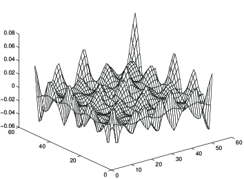
Figure 1: Eigenmode of level 1.

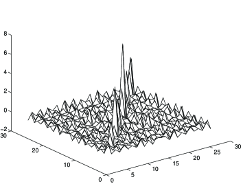
Figure 2: Stable waveleton pattern.

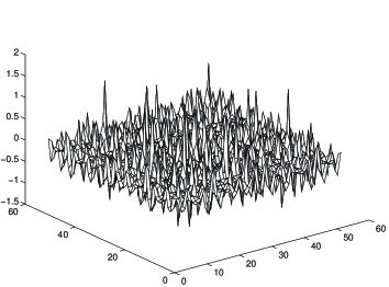
Figure 3: Chaotic-like behaviour.

Formula (18) gives us expansion into the slow part $\Psi_{N,M}^{slow}$ and fast oscillating parts for arbitrary N, M. So, we may move from coarse scales of resolution to the finest one for obtaining more detailed information about our dynamical process. The first terms in the RHS of formulae (18) correspond on the global level of function space decomposition to resolution space and the second ones to detail space. It should be noted that such representations give the best possible localization properties in the corresponding (phase)space/time coordinates. In contrast with different approaches formulae (18) do not use perturbation technique or linearization procedures. So, by using wavelet bases with their good (phase) space/time localization properties we can describe high-localized (coherent) structures in spatially-extended stochastic systems with collective behaviour. Modelling demonstrates the appearance of stable patterns formation from high-localized coherent structures or chaotic behaviour. On Fig. 1 we present contribution to the full expansion from coarsest level (waveleton) of decomposition (18). Fig. 2, 3 show the representations for full solutions, constructed from the first 6 eigenmodes (6 levels in formula (18)), and demonstrate stable localized pattern formation and chaotic-like behaviour outside of KAM region. We can control the type of behaviour on the level of reduced algebraical system (16).

References

- [1] R. C. Davidson, e.a., Phys. Rev. ST AB, 4, 104401, 2001.
- [2] R.C. Davidson, e.a., Phys. Rev. ST AB, 3, 084401, 2000.
- [3] A.N. Fedorova and M.G. Zeitlin, Math. and Comp. in Simulation, 46, 527, 1998.
- [4] A.N. Fedorova and M.G. Zeitlin, New Applications of Nonlinear and Chaotic Dynamics in Mechanics, 31, 101 Kluwer, 1998.
- [5] A.N. Fedorova and M.G. Zeitlin, CP405, 87, American Institute of Physics, 1997. Los Alamos preprint, physics/9710035.
- [6] A.N. Fedorova, M.G. Zeitlin and Z. Parsa, Proc. PAC97 2, 1502, 1505, 1508, APS/IEEE, 1998.
- [7] A.N. Fedorova, M.G. Zeitlin and Z. Parsa, Proc. EPAC98, 930, 933, Institute of Physics, 1998.
- [8] A.N. Fedorova, M.G. Zeitlin and Z. Parsa, CP468, 48, American Institute of Physics, 1999. Los Alamos preprint, physics/990262.
- [9] A.N. Fedorova, M.G. Zeitlin and Z. Parsa, CP468, 69, American Institute of Physics, 1999. Los Alamos preprint, physics/990263.
- [10] A.N. Fedorova and M.G. Zeitlin, Proc. PAC99, 1614, 1617, 1620, 2900, 2903, 2906, 2909, 2912, APS/IEEE, New York, 1999. Los Alamos preprints: physics/9904039, 9904040, 9904041, 9904042, 9904043, 9904045, 9904046, 9904047.
- [11] A.N. Fedorova and M.G. Zeitlin, The Physics of High Brightness Beams, 235, World Scientific, 2000. Los Alamos preprint: physics/0003095.
- [12] A.N. Fedorova and M.G. Zeitlin, Proc. EPAC00, 415, 872, 1101, 1190, 1339, 2325, Austrian Acad.Sci.,2000. Los Alamos preprints: physics/0008045, 0008046, 0008047, 0008048, 0008049, 0008050.
- [13] A.N. Fedorova, M.G. Zeitlin, Proc. 20 International Linac Conf., 300, 303, SLAC, Stanford, 2000. Los Alamos preprints: physics/0008043, 0008200.
- [14] A.N. Fedorova, M.G. Zeitlin, Los Alamos preprints: physics/0101006, 0101007 and World Scientific, in press.
- [15] A.N. Fedorova, M.G. Zeitlin, Proc. PAC2001, Chicago, 790-1792, 1805-1807, 1808-1810, 1811-1813, 1814-1816, 2982-2984, 3006-3008, IEEE, 2002 or arXiv preprints: physics/0106022, 0106010, 0106009, 0106008, 0106007, 0106006, 0106005.
- [16] A.N. Fedorova, M.G. Zeitlin, Proc. in Applied Mathematics and Mechanics, 1, Issue 1, pp. 399-400, 432-433, Wiley-VCH, 2002.
- [17] A.N. Fedorova, M.G. Zeitlin, this Proc.