COLLECTIVE DYNAMICAL MODELS

OF BEAM/PLASMA PHYSICS

Antonina N. Fedorova, Michael G. Zeitlin

IPME RAS, St. Petersburg, V.O. Bolshoj pr., 61, 199178, Russia

e-mail: zeitlin@math.ipme.ru

http://www.ipme.ru/zeitlin.html

http://www.ipme.nw.ru/zeitlin.html FAST CALCULATION METHODS IN COLLECTIVE DYNAMICAL MODELS OF BEAM/PLASMA PHYSICS Antonina N. Fedorova    Michael G. Zeitlin IPME RAS    St. Petersburg    V.O. Bolshoj pr    61    199178    Russia e-mail: zeitlin@math.ipme.ruhttp://www.ipme.ru/zeitlin.html; http://www.ipme.nw.ru/zeitlin.html Abstract We consider an application of modification of our variational-wavelet approach to some nonlinear collective model of beam/plasma physics: Vlasov/Boltzmann-like reduction from general BBGKY hierachy related to modeling of propagation of intense charged particle beams in high-intensity accelerators and transport systems. We use fast convergent multiscale variational-wavelet representations for solutions which allow to consider polynomial and rational type of nonlinearities. The solutions are represented via the multiscale decomposition in nonlinear high-localized eigenmodes (waveletons). In contrast with different approaches we do not use perturbation technique or linearization procedures. Abstract We consider an application of modification of our variational-wavelet approach to some nonlinear collective model of beam/plasma physics: Vlasov/Boltzmann-like reduction from general BBGKY hierachy related to modeling of propagation of intense charged particle beams in high-intensity accelerators and transport systems. We use fast convergent multiscale variational-wavelet representations for solutions which allow to consider polynomial and rational type of nonlinearities. The solutions are represented via the multiscale decomposition in nonlinear high-localized eigenmodes (waveletons). In contrast with different approaches we do not use perturbation technique or linearization procedures. Presented at the Eighth European Particle Accelerator Conference

EPAC’02

Paris, France, June 3-7, 2002

1 INTRODUCTION

We consider applications of numerical–analytical technique based on modification of our variational-wavelet approach to nonlinear collective models of beam/plasma physics, e.g. some forms of Vlasov/Boltzmann-like reductions from general BBGKY hierarchy (section 2). These equations are related to the modeling of propagation of intense charged particle beams in high-intensity accelerators and transport systems [1], [2]. In our approach we use fast convergent multiscale variational-wavelet representations, which allows to consider polynomial and rational type of nonlinearities [3]-[16], [17]. The solutions are represented via the multiscale decomposition in nonlinear high-localized eigenmodes (generalized Gluckstern modes, in some sense), which corresponds to the full multiresolution expansion in all underlying hidden time/space or phase space scales. In contrast with different approaches we don’t use perturbation technique or linearization procedures. In section 3 after formulation of key points we consider another variational approach based on ideas of para-products and nonlinear approximation in multiresolution approach, which gives the possibility for computations in each scale separately [18]. We consider representation (4) below, where each term corresponds to the contribution from the scale $i$ in the full underlying multiresolution decomposition as multiscale generalization of old (nonlinear) $\delta F$ approach [1]. As a result, fast scalar/parallel modeling demonstrates appearance of high-localized coherent structures (waveletons) and pattern formation in systems with complex collective behaviour.

2 VLASOV/BOLTZMANN–LIKE REDUCTIONS

Let M be the phase space of ensemble of N particles (${\rm dim}M=6N$) with coordinates $x_{i}=(q_{i},p_{i}),\quad i=1,...,N,\quad q_{i}=(q^{1}_{i},q^{2}_{i},q^{3}_{i})\in R^{3},\quad p_{i}=(p^{1}_{i},p^{2}_{i},p^{3}_{i})\in R^{3}$ with distribution function $D_{N}(x_{1},\dots,x_{N};t)$ and

$$F_{N}(x_{1},\dots,x_{N};t)=\sum_{S_{N}}D_{N}(x_{1},\dots,x_{N};t)$$ (1)

be the N-particle distribution functions ($S_{N}$ is permutation group of N elements). For s=1,2 we have from general BBGKY hierarchy:

$$\frac{\partial F_{1}(x_{1};t)}{\partial t}+\frac{p_{1}}{m}\frac{\partial}{\partial q_{1}}F_{1}(x_{1};t)$$ (2)

$$=\frac{1}{\upsilon}\int\mathrm{d}x_{2}L_{12}F_{2}(x_{1},x_{2};t)$$

$$\frac{\partial F_{2}(x_{1},x_{2};t)}{\partial t}+\Big{(}\frac{p_{1}}{m}\frac{\partial}{\partial q_{1}}+\frac{p_{2}}{m}\frac{\partial}{\partial q_{2}}-L_{12}\Big{)}$$ (3)

$$F_{2}(x_{1},x_{2};t)=\frac{1}{\upsilon}\int\mathrm{d}x_{3}(L_{13}+L_{23})F_{3}(x_{1},x_{2};t)$$

where partial Liouvillean operators are described in [17]. We are interested in the cases when F_k(x_1,…,x_k;t)=∏^k_i=1F_1(x_i;t)+G_k(x_1,…,x_k;t), where $G_{k}$ are correlation patterns, really have additional reductions as in case of Vlasov-like systems. Then we have in (2), (3) polynomial type of nonlinearities (more exactly, multilinearities).

3 MULTISCALE ANALYSIS

Our goal is the demonstration of advantages of the following representation

$$F=\sum_{i\in Z}\delta^{i}F,$$ (4)

for the full exact solution for the systems related to equations (2), (3). It is possible to consider (4) as multiscale generalization of old (nonlinear) $\delta F$ approach [1]. In (4) each $\delta^{i}F$ term corresponds to the contribution from the scale $i$ in the full underlying multiresolution decomposition

$$\dots\subset V_{-1}\subset V_{0}\subset V_{1}\subset V_{2}\dots$$ (5)

of the proper function space ($L^{2}$, Hilbert, Sobolev, etc) to which $F$ is really belong. It should be noted that (4) doesn’t based neither on perturbations nor on linearization procedures. Although usually physicists, who prefered computer modelling as a main tool of understanding of physical reality, don’t think about underlying functional spaces, but many concrete features of complicated complex dynamics are really related not only to concrete form/class of operators/equations but also depend on the proper choice of function spaces where operators actully act. Moreover, we have for arbitrary $N$ in the finite N-mode approximation

$$F^{N}=\sum^{N}_{i=1}\delta^{i}F$$ (6)

the following more useful decompositions:

$$\{F(t)\}=\bigoplus_{-\infty<j<\infty}W_{j}\quad{\rm or}\quad\{F(t)\}=\overline{V_{0}\displaystyle\bigoplus^{\infty}_{j=0}W_{j}},$$ (7)

in case when $V_{0}$ is the coarsest scale of resolution and where $V_{j+1}=V_{j}\bigoplus W_{j}$ and bases in scale spaces $W_{i}(V_{j})$ are generated from base functions $\psi(\varphi)$ by action of affine group of translations and dilations (the so called “wavelet microscope”). The following constructions based on variational approach provide the best possible fast convergence properties in the sense of combined norm

$$\|F^{N+1}-F^{N}\|\leq\varepsilon$$ (8)

introduced in [17]. Our five basic points after functional space choice are:

1. Ansatz-oriented choice of the (multidimensional) bases related to some polynomial tensor algebra. Some example related to general BBGKY hierarchy is considered in [17].

2. The choice of proper variational principle. A few projection/ Galerkin-like principles for constructing (weak) solutions are considered in [3] - [16]. It should be noted advantages of formulations related to biorthogonal (wavelet) decomposition.

3. The choice of bases functions in scale spaces $W_{j}$ from wavelet zoo. They correspond to high-localized (nonlinear) oscillations/excitations, coherent (nonlinear) resonances, etc. Besides fast convergence properties of the corresponding variational-wavelet expansions it should be noted minimal complexity of all underlying calculations, especially in case of choice of wavelet packets which minimize Shannon entropy.

4. Operators representations providing maximum sparse representations for arbitrary (pseudo) differential/ integral operators $\mathrm{d}f/\mathrm{d}x,\mathrm{d}^{n}f/\mathrm{d}x^{n},\int T(x,y)f(y)\mathrm{d}y)$, etc [17].

5. (Multi)linearization. Besides variation approach we consider now a different method to deal with (polynomial) nonlinearities.

We modify the scheme of our variational approach in such a way in which we consider different scales of multiresolution decomposition (5) separately. For this reason we need to compute errors of approximations. The main problems come of course from nonlinear (polynomial) terms. We follow according to the multilinearization (in case below – bilinearization) approach of Beylkin, Meyer etc from [18]. Let $P_{j}$ be projection operators on the subspaces $V_{j}$ (5):

$$(P_{j}f)(x)=\sum_{k}<f,\varphi_{j,k}>\varphi_{j,k}(x)$$ (9)

and $Q_{j}$ are projection operators on the subspaces $W_{j}$: $Q_{j}=P_{j-1}-P_{j}$. So, for $u\in L^{2}(R)$ we have $u_{j}=P_{j}u\quad$ and $u_{j}\in V_{j}$. It is obviously that we can represent $u_{0}^{2}$ in the following form:

$$u_{0}^{2}=2\sum^{n}_{j=1}(P_{j}u)(Q_{j}u)+\sum^{n}_{j=1}(Q_{j}u)(Q_{j}u)+u_{n}^{2}$$ (10)

In this formula there is no interaction between different scales. We may consider each term of (10) as a bilinear mappings:

$$\displaystyle M_{VW}^{j}:V_{j}\times W_{j}\to L^{2}({\bf R})=V_{j}{\oplus_{j^{\prime}\geq j}W_{j^{\prime}}}$$ (11)

$$M_{WW}^{j}:W_{j}\times W_{j}\to L^{2}({\bf R})=V_{j}\oplus_{j^{\prime}\geq j}W_{j^{\prime}}$$ (12)

For numerical purposes we need formula (10) with a finite number of scales, but when we consider limits $j\to\infty$ we have

$$u^{2}=\sum_{j\in{\bf Z}}(2P_{j}u+Q_{j}u)(Q_{j}u),$$ (13)

which is para-product of Bony, Coifman and Meyer [18]. Now we need to expand (10) into the wavelet bases. To expand each term in (10) we need to consider the integrals of the products of the basis functions (7), e.g.

$$M^{j,j^{\prime}}_{WWW}(k,k^{\prime},\ell)=\int^{\infty}_{-\infty}\psi^{j}_{k}(x)\psi^{j}_{k^{\prime}}(x)\psi^{j^{\prime}}_{\ell}(x)\mathrm{d}x,$$ (14)

where $j^{\prime}>j$ and

$$\psi^{j}_{k}(x)=2^{-j/2}\psi(2^{-j}x-k)$$ (15)

are the basis functions (7). For compactly supported wavelets

$$M_{WWW}^{j,j^{\prime}}(k,k^{\prime},\ell)\equiv 0\quad\mbox{for}\quad|k-k^{\prime}|>k_{0},$$ (16)

where $k_{0}$ depends on the overlap of the supports of the basis functions and

$$|M_{WWW}^{r}(k-k^{\prime},2^{r}k-\ell)|\leq C\cdot 2^{-r\lambda M}$$ (17)

Let us define $j_{0}$ as the distance between scales such that for a given $\varepsilon$ all the coefficients in (17) with labels $r=j-j^{\prime}$, $r>j_{0}$ have absolute values less than $\varepsilon$.

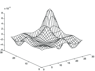
Figure 1: $N=1$ waveleton contribution to (6).

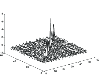
Figure 2: Stable pattern.

For the purposes of computing with accuracy $\varepsilon$ we replace the mappings in (11), (12) by

$$M_{VW}^{j}:V_{j}\times W_{j}\to V_{j}\oplus_{j\leq j^{\prime}\leq j_{0}}W_{j^{\prime}}$$ (18)

$$M_{WW}^{j}:W_{j}\times W_{j}\to V_{j}\oplus_{j\leq j^{\prime}\leq j_{0}}W_{j^{\prime}}$$

Since $V_{j}\oplus_{j\leq j^{\prime}\leq j_{0}}W_{j^{\prime}}=V_{j_{0}-1},\ V_{j}\subset V_{j_{0}-1},\ W_{j}\subset V_{j_{0}-1}$ we may consider bilinear mappings (18), (3) on $V_{j_{0}-1}\times V_{j_{0}-1}$. For the evaluation of (18), (3) as mappings $V_{j_{0}-1}\times V_{j_{0}-1}\to V_{j_{0}-1}$ we need significantly fewer coefficients than for mappings (18), (3). It is enough to consider only coefficients

$$M(k,k^{\prime},\ell)=2^{-j/2}\int^{\infty}_{\infty}\varphi(x-k)\varphi(x-k^{\prime})\varphi(x-\ell)\mathrm{d}x,$$ (19)

where $\varphi(x)$ is scale function. Also we have

$$M(k,k^{\prime},\ell)=2^{-j/2}M_{0}(k-\ell,k^{\prime}-\ell),$$ (20)

where

$$M_{0}(p,q)=\int\varphi(x-p)\varphi(x-q)\varphi(x)\mathrm{d}x$$ (21)

$M_{0}(p,q)$ satisfy the standard system of linear equations and after its solution we can recover all bilinear quantities (14). Then we apply some variation approach from [3]-[16], but in each scale separately. So, after application of points 1-5 above, we arrive to explicit numerical-analytical realization of representations (4) or (6). Fig.1 demonstrates the first contribution to the full solution (6) while Fig.2 presents (stable) pattern as solution of system (2)-(3). We evaluate accuracy of calculations according to norm introduced in [17].

References

- [1] R.C. Davidson, e.a., Phys. Plasmas, 6, 298, 1999
- [2] The Physics of High Brightness Beams, Ed.J. Rosenzweig & L. Serafini, World Scientific, 2000.
- [3] A.N. Fedorova and M.G. Zeitlin, Math. and Comp. in Simulation, 46, 527, 1998.
- [4] A.N. Fedorova and M.G. Zeitlin, New Applications of Nonlinear and Chaotic Dynamics in Mechanics, 31, 101 Kluwer, 1998.
- [5] A.N. Fedorova and M.G. Zeitlin, CP405, 87, American Institute of Physics, 1997. Los Alamos preprint, physics/9710035.
- [6] A.N. Fedorova, M.G. Zeitlin and Z. Parsa, Proc. PAC97 2, 1502, 1505, 1508, APS/IEEE, 1998.
- [7] A.N. Fedorova, M.G. Zeitlin and Z. Parsa, Proc. EPAC98, 930, 933, Institute of Physics, 1998.
- [8] A.N. Fedorova, M.G. Zeitlin and Z. Parsa, CP468, 48, American Institute of Physics, 1999. Los Alamos preprint, physics/990262.
- [9] A.N. Fedorova, M.G. Zeitlin and Z. Parsa, CP468, 69, American Institute of Physics, 1999. Los Alamos preprint, physics/990263.
- [10] A.N. Fedorova and M.G. Zeitlin, Proc. PAC99, 1614, 1617, 1620, 2900, 2903, 2906, 2909, 2912, APS/IEEE, New York, 1999. Los Alamos preprints: physics/9904039, 9904040, 9904041, 9904042, 9904043, 9904045, 9904046, 9904047.
- [11] A.N. Fedorova and M.G. Zeitlin, The Physics of High Brightness Beams, 235, World Scientific, 2000. Los Alamos preprint: physics/0003095.
- [12] A.N. Fedorova and M.G. Zeitlin, Proc. EPAC00, 415, 872, 1101, 1190, 1339, 2325, Austrian Acad.Sci.,2000. Los Alamos preprints: physics/0008045, 0008046, 0008047, 0008048, 0008049, 0008050.
- [13] A.N. Fedorova, M.G. Zeitlin, Proc. 20 International Linac Conf., 300, 303, SLAC, Stanford, 2000. Los Alamos preprints: physics/0008043, 0008200.
- [14] A.N. Fedorova, M.G. Zeitlin, Los Alamos preprints: physics/0101006, 0101007 and World Scientific, in press.
- [15] A.N. Fedorova, M.G. Zeitlin, Proc. PAC2001, Chicago, 790-1792, 1805-1807, 1808-1810, 1811-1813, 1814-1816, 2982-2984, 3006-3008, IEEE, 2002 or arXiv preprints: physics/0106022, 0106010, 0106009, 0106008, 0106007, 0106006, 0106005.
- [16] A.N. Fedorova, M.G. Zeitlin, Proc. in Applied Mathematics and Mechanics, Volume 1, Issue 1, pp. 399-400, 432-433, Wiley-VCH, 2002.
- [17] A.N. Fedorova, M.G. Zeitlin, this Proc.
- [18] Beylkin, G., Colorado preprint, 1992; Y. Meyer, Wavelets and Operators, 1990