IN BBGKY COLLECTIVE DYNAMICS Antonina N. Fedorova, Michael G. Zeitlin

IPME RAS, St. Petersburg, V.O. Bolshoj pr., 61, 199178, Russia

e-mail: zeitlin@math.ipme.ru

http://www.ipme.ru/zeitlin.html

http://www.ipme.nw.ru/zeitlin.html FROM LOCALIZATION TO STOCHASTICS IN BBGKY COLLECTIVE DYNAMICS Antonina N. Fedorova    Michael G. Zeitlin IPME RAS    St. Petersburg    V.O. Bolshoj pr    61    199178    Russia e-mail: zeitlin@math.ipme.ruhttp://www.ipme.ru/zeitlin.html; http://www.ipme.nw.ru/zeitlin.html Abstract Fast and efficient numerical-analytical approach is proposed for modeling complex collective behaviour in accelerator/plasma physics models based on BBGKY hierarchy of kinetic equations. Our calculations are based on variational and multiresolution approaches in the bases of polynomial tensor algebras of generalized coherent states/wavelets. We construct the representation for hierarchy of reduced distribution functions via the multiscale decomposition in high-localized eigenmodes. Numerical modeling shows the creation of different internal coherent structures from localized modes, which are related to stable/unstable type of behaviour and corresponding pattern (waveletons) formation. Abstract Fast and efficient numerical-analytical approach is proposed for modeling complex collective behaviour in accelerator/plasma physics models based on BBGKY hierarchy of kinetic equations. Our calculations are based on variational and multiresolution approaches in the bases of polynomial tensor algebras of generalized coherent states/wavelets. We construct the representation for hierarchy of reduced distribution functions via the multiscale decomposition in high-localized eigenmodes. Numerical modeling shows the creation of different internal coherent structures from localized modes, which are related to stable/unstable type of behaviour and corresponding pattern (waveletons) formation. Presented at the Eighth European Particle Accelerator Conference

EPAC’02

Paris, France, June 3-7, 2002

1 INTRODUCTION

The kinetic theory describes a lot of phenomena in beam/plasma physics which cannot be understood on the thermodynamic or/and fluid models level. We mean first of all (local) fluctuations from equilibrium state and collective/relaxation phenomena. It is well-known that only kinetic approach can describe Landau damping, intra-beam scattering, while Schottky noise and associated cooling technique depend on the understanding of spectrum of local fluctuations of the beam charge density [1]. In this paper we consider the applications of a new numericalanalytical technique based on wavelet analysis approach for calculations related to description of complex collective behaviour in the framework of general BBGKY hierarchy. The rational type of nonlinearities allows us to use our results from [2]-[15], which are based on the application of wavelet analysis technique and variational formulation of initial nonlinear problems. Wavelet analysis is a set of mathematical methods which give us a possibility to work with well-localized bases in functional spaces and provide maximum sparse forms for the general type of operators (differential, integral, pseudodifferential) in such bases. It provides the best possible rates of convergence and minimal complexity of algorithms inside and as a result saves CPU time and HDD space. In part 2 set-up for kinetic BBGKY hierarchy is described. In part 3 we present explicit analytical construction for solutions of hierarchy of equations from part 2, which is based on tensor algebra extensions of multiresolution representation and variational formulation. We give explicit representation for hierarchy of n-particle reduced distribution functions in the base of high-localized generalized coherent (regarding underlying affine group) states given by polynomial tensor algebra of wavelets, which takes into account contributions from all underlying hidden multiscales from the coarsest scale of resolution to the finest one to provide full information about stochastic dynamical process. So, our approach resembles Bogolubov and related approaches but we don’t use any perturbation technique (like virial expansion) or linearization procedures. Numerical modeling shows the creation of different internal (coherent) structures from localized modes, which are related to stable (equilibrium) or unstable type of behaviour and corresponding pattern (waveletons) formation.

2 BBGKY HIERARCHY

Let M be the phase space of ensemble of N particles (${\rm dim}M=6N$) with coordinates $x_{i}=(q_{i},p_{i}),\quad i=1,...,N,\quad q_{i}=(q^{1}_{i},q^{2}_{i},q^{3}_{i})\in R^{3},\quad p_{i}=(p^{1}_{i},p^{2}_{i},p^{3}_{i})\in R^{3},\quad q=(q_{1},\dots,q_{N})\in R^{3N}$. Individual and collective measures are:

$$\mu_{i}=\mathrm{d}x_{i}=\mathrm{d}q_{i}p_{i},\quad\mu=\prod^{N}_{i=1}\mu_{i}$$ (1)

Distribution function $D_{N}(x_{1},\dots,x_{N};t)$ satisfies Liouville equation of motion for ensemble with Hamiltonian $H_{N}$ :

$$\frac{\partial D_{N}}{\partial t}=\{H_{N},D_{N}\}$$ (2)

and normalization constraint

$$\int D_{N}(x_{1},\dots,x_{N};t)\mathrm{d}\mu=1$$ (3)

where Poisson brackets are:

$$\{H_{N},D_{N}\}=\sum^{N}_{i=1}\Big{(}\frac{\partial H_{N}}{\partial q_{i}}\frac{\partial D_{N}}{\partial p_{i}}-\frac{\partial H_{N}}{\partial p_{i}}\frac{\partial D_{N}}{\partial q_{i}}\Big{)}$$ (4)

Our constructions can be applied to the following general Hamiltonians:

$$H_{N}=\sum^{N}_{i=1}\Big{(}\frac{p^{2}_{i}}{2m}+U_{i}(q)\Big{)}+\sum_{1\leq i\leq j\leq N}U_{ij}(q_{i},q_{j})$$ (5)

where potentials $U_{i}(q)=U_{i}(q_{1},\dots,q_{N})$ and $U_{ij}(q_{i},q_{j})$ are not more than rational functions on coordinates. Let $L_{s}$ and $L_{ij}$ be the Liouvillean operators (vector fields)

$$L_{s}=\sum^{s}_{j=1}\Big{(}\frac{p_{j}}{m}\frac{\partial}{\partial q_{j}}-\frac{\partial u_{j}}{\partial q}\frac{\partial}{\partial p_{j}}\Big{)}-\sum_{1\leq i\leq j\leq s}L_{ij}$$ (6)

$$L_{ij}=\frac{\partial U_{ij}}{\partial q_{i}}\frac{\partial}{\partial p_{i}}+\frac{\partial U_{ij}}{\partial q_{j}}\frac{\partial}{\partial p_{j}}$$ (7)

For s=N we have the following representation for Liouvillean vector field

$$L_{N}=\{H_{N},\cdot\}$$ (8)

and the corresponding ensemble equation of motion:

$$\frac{\partial D_{N}}{\partial t}+L_{N}D_{N}=0$$ (9)

$L_{N}$ is self-adjoint operator regarding standard pairing on the set of phase space functions. Let

$$F_{N}(x_{1},\dots,x_{N};t)=\sum_{S_{N}}D_{N}(x_{1},\dots,x_{N};t)$$ (10)

be the N-particle distribution function ($S_{N}$ is permutation group of N elements). Then we have the hierarchy of reduced distribution functions ($V^{s}$ is the corresponding normalized volume factor)

$$F_{s}(x_{1},\dots,x_{s};t)=$$ (11)

$$V^{s}\int D_{N}(x_{1},\dots,x_{N};t)\prod_{s+1\leq i\leq N}\mu_{i}$$

After standard manipulations we arrived to BBGKY hierarchy [1]:

$$\frac{\partial F_{s}}{\partial t}+L_{s}F_{s}=\frac{1}{\upsilon}\int\mathrm{d}\mu_{s+1}\sum^{s}_{i=1}L_{i,s+1}F_{s+1}$$ (12)

It should be noted that we may apply our approach even to more general formulation than (12). Some particular case is considered in [16].

3 MULTISCALE ANALYSIS

The infinite hierarchy of distribution functions satisfying system (12) in the thermodynamical limit is:

$$F=\{F_{0},F_{1}(x_{1};t),F_{2}(x_{1},x_{2};t),\dots,$$ (13)

$$F_{N}(x_{1},\dots,x_{N};t),\dots\}$$

where $F_{p}(x_{1},\dots,x_{p};t)\in H^{p}$, $H^{0}=R,\quad H^{p}=L^{2}(R^{6p})$ (or any different proper functional space), $F\in$ $H^{\infty}=H^{0}\oplus H^{1}\oplus\dots\oplus H^{p}\oplus\dots$ with the natural Fock-space like norm (of course, we keep in mind the positivity of the full measure):

$$(F,F)=F^{2}_{0}+\sum_{i}\int F^{2}_{i}(x_{1},\dots,x_{i};t)\prod^{i}_{\ell=1}\mu_{\ell}$$ (14)

First of all we consider $F=F(t)$ as function on time variable only, $F\in L^{2}(R)$, via multiresolution decomposition which naturally and efficiently introduces the infinite sequence of underlying hidden scales into the game [17]. Because affine group of translations and dilations is inside the approach, this method resembles the action of a microscope. We have contribution to final result from each scale of resolution from the whole infinite scale of spaces. Let the closed subspace $V_{j}(j\in{\bf Z})$ correspond to level j of resolution, or to scale j. We consider a multiresolution analysis of $L^{2}(R)$ (of course, we may consider any different functional space) which is a sequence of increasing closed subspaces $V_{j}$: $...V_{-2}\subset V_{-1}\subset V_{0}\subset V_{1}\subset V_{2}\subset...$ satisfying the following properties: let $W_{j}$ be the orthonormal complement of $V_{j}$ with respect to $V_{j+1}$: $V_{j+1}=V_{j}\bigoplus W_{j}$ then we have the following decomposition:

$$\{F(t)\}=\bigoplus_{-\infty<j<\infty}W_{j}$$ (15)

or in case when $V_{0}$ is the coarsest scale of resolution:

$$\{F(t)\}=\overline{V_{0}\displaystyle\bigoplus^{\infty}_{j=0}W_{j}},$$ (16)

Subgroup of translations generates basis for fixed scale number: ${\rm span}_{k\in Z}\{2^{j/2}\Psi(2^{j}t-k)\}=W_{j}.$ The whole basis is generated by action of full affine group:

$${\rm span}_{k\in Z,j\in Z}\{2^{j/2}\Psi(2^{j}t-k)\}=$$ (17)

$${\rm span}_{k,j\in Z}\{\Psi_{j,k}\}=\{F(t)\}$$

Let sequence $\{V_{j}^{t}\},V_{j}^{t}\subset L^{2}(R)$ correspond to multiresolution analysis on time axis, $\{V_{j}^{x_{i}}\}$ correspond to multiresolution analysis for coordinate $x_{i}$, then

$$V_{j}^{n+1}=V^{x_{1}}_{j}\otimes\dots\otimes V^{x_{n}}_{j}\otimes V^{t}_{j}$$ (18)

corresponds to multiresolution analysis for n-particle distribution fuction $F_{n}(x_{1},\dots,x_{n};t)$. E.g., for $n=2$:

$$V^{2}_{0}=\{f:f(x_{1},x_{2})=$$ (19)

$$\sum_{k_{1},k_{2}}a_{k_{1},k_{2}}\phi^{2}(x_{1}-k_{1},x_{2}-k_{2}),\ a_{k_{1},k_{2}}\in\ell^{2}(Z^{2})\},$$

where $\phi^{2}(x_{1},x_{2})=\phi^{1}(x_{1})\phi^{2}(x_{2})=\phi^{1}\otimes\phi^{2}(x_{1},x_{2}),$ and $\phi^{i}(x_{i})\equiv\phi(x_{i})$ form a multiresolution basis corresponding to $\{V_{j}^{x_{i}}\}$. If $\{\phi^{1}(x_{1}-\ell)\},\ \ell\in Z$ form an orthonormal set, then $\phi^{2}(x_{1}-k_{1},x_{2}-k_{2})$ form an orthonormal basis for $V^{2}_{0}$. Action of affine group provides us by multiresolution representation of $L^{2}(R^{2})$. After introducing detail spaces $W^{2}_{j}$, we have, e.g. $V^{2}_{1}=V^{2}_{0}\oplus W^{2}_{0}.$ Then 3-component basis for $W^{2}_{0}$ is generated by translations of three functions

$$\Psi^{2}_{1}=\phi^{1}(x_{1})\otimes\Psi^{2}(x_{2}),\ \Psi^{2}_{2}=\Psi^{1}(x_{1})\otimes\phi^{2}(x_{2}),$$

$$\Psi^{2}_{3}=\Psi^{1}(x_{1})\otimes\Psi^{2}(x_{2})$$ (20)

Also, we may use the rectangle lattice of scales and one-dimentional wavelet decomposition : f(x_1,x_2)=∑_i,ℓ;j,k¡f,Ψ_i,ℓ⊗Ψ_j,k¿ Ψ_j,ℓ⊗Ψ_j,k(x_1,x_2) where bases functions $\Psi_{i,\ell}\otimes\Psi_{j,k}$ depend on two scales $2^{-i}$ and $2^{-j}$. After constructing multidimension bases we apply one of variational procedures from [2]-[16]. As a result the solution of equations (12) has the following multiscale/multiresolution decomposition via nonlinear high-localized eigenmodes

$$F(t,x_{1},x_{2},\dots)=\sum_{(i,j)\in Z^{2}}a_{ij}U^{i}\otimes V^{j}(t,x_{1},x_{2},\dots)$$

$$V^{j}(t)=V_{N}^{j,slow}(t)+\sum_{l\geq N}V^{j}_{l}(\omega_{l}t),\quad\omega_{l}\sim 2^{l}$$ (21)

$$U^{i}(x_{s})=U_{M}^{i,slow}(x_{s})+\sum_{m\geq M}U^{i}_{m}(k^{s}_{m}x_{s}),\quad k^{s}_{m}\sim 2^{m},$$

which corresponds to the full multiresolution expansion in all underlying time/space scales.

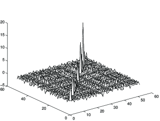
Figure 1: 6-eigenmodes representation.

Formulae (21) give us expansion into the slow part $\Psi_{N,M}^{slow}$ and fast oscillating parts for arbitrary N, M. So, we may move from coarse scales of resolution to the finest one for obtaining more detailed information about our dynamical process. The first terms in the RHS of formulae (21) correspond on the global level of function space decomposition to resolution space and the second ones to detail space. In this way we give contribution to our full solution from each scale of resolution or each time/space scale or from each nonlinear eigenmode. It should be noted that such representations give the best possible localization properties in the corresponding (phase)space/time coordinates. In contrast with different approaches formulae (21) do not use perturbation technique or linearization procedures. Numerical calculations are based on compactly supported wavelets and related wavelet families and on evaluation of the accuracy regarding norm (14):

$$\|F^{N+1}-F^{N}\|\leq\varepsilon$$ (22)

Fig. 1 demonstrates 6-scale/eigenmodes (waveletons) construction for solution of equations like (12). So, by using wavelet bases with their good (phase) space/time localization properties we can construct high-localized waveleton structures in spatially-extended stochastic systems with collective behaviour.

References

- [1] A. W. Chao, Physics of Collective Beam Instabilities in High Energy Accelerators, Wiley, 1993
- [2] A.N. Fedorova and M.G. Zeitlin, Math. and Comp. in Simulation, 46, 527, 1998.
- [3] A.N. Fedorova and M.G. Zeitlin, New Applications of Nonlinear and Chaotic Dynamics in Mechanics, 31, 101 Kluwer, 1998.
- [4] A.N. Fedorova and M.G. Zeitlin, CP405, 87, American Institute of Physics, 1997. Los Alamos preprint, physics/9710035.
- [5] A.N. Fedorova, M.G. Zeitlin and Z. Parsa, Proc. PAC97 2, 1502, 1505, 1508, APS/IEEE, 1998.
- [6] A.N. Fedorova, M.G. Zeitlin and Z. Parsa, Proc. EPAC98, 930, 933, Institute of Physics, 1998.
- [7] A.N. Fedorova, M.G. Zeitlin and Z. Parsa, CP468, 48, American Institute of Physics, 1999. Los Alamos preprint, physics/990262.
- [8] A.N. Fedorova, M.G. Zeitlin and Z. Parsa, CP468, 69, American Institute of Physics, 1999. Los Alamos preprint, physics/990263.
- [9] A.N. Fedorova and M.G. Zeitlin, Proc. PAC99, 1614, 1617, 1620, 2900, 2903, 2906, 2909, 2912, APS/IEEE, New York, 1999. Los Alamos preprints: physics/9904039, 9904040, 9904041, 9904042, 9904043, 9904045, 9904046, 9904047.
- [10] A.N. Fedorova and M.G. Zeitlin, The Physics of High Brightness Beams, 235, World Scientific, 2000. Los Alamos preprint: physics/0003095.
- [11] A.N. Fedorova and M.G. Zeitlin, Proc. EPAC00, 415, 872, 1101, 1190, 1339, 2325, Austrian Acad.Sci.,2000. Los Alamos preprints: physics/0008045, 0008046, 0008047, 0008048, 0008049, 0008050.
- [12] A.N. Fedorova, M.G. Zeitlin, Proc. 20 International Linac Conf., 300, 303, SLAC, Stanford, 2000. Los Alamos preprints: physics/0008043, 0008200.
- [13] A.N. Fedorova, M.G. Zeitlin, Los Alamos preprints: physics/0101006, 0101007 and World Scientific, in press.
- [14] A.N. Fedorova, M.G. Zeitlin, Proc. PAC2001, Chicago, 790-1792, 1805-1807, 1808-1810, 1811-1813, 1814-1816, 2982-2984, 3006-3008, IEEE, 2002 or arXiv preprints: physics/0106022, 0106010, 0106009, 0106008, 0106007, 0106006, 0106005.
- [15] A.N. Fedorova, M.G. Zeitlin, Proc. in Applied Mathematics and Mechanics, Volume 1, Issue 1, pp. 399-400, 432-433, Wiley-VCH, 2002.
- [16] A.N. Fedorova, M.G. Zeitlin, this Proc.
- [17] Y. Meyer, Wavelets and Operators, CUP, 1990