Spontaneous emission rate of an excited atom
placed near a nanofiber

Abstract

The spontaneous decay rates of an excited atom placed near a dielectric cylinder are investigated. A special attention is paid to the case when the cylinder radius is small in comparison with radiation wavelength (nanofiber or photonic wire). In this case, the analytical expressions of the transition rates for different orientations of dipole are derived. It is shown that the main contribution to decay rates is due to quasistatic interaction of atom dipole momentum with nanofiber and the contributions of guided modes are exponentially small. On the contrary, in the case when the radius of fiber is only slightly less than radiation wavelength, the influence of guided modes can be substantial. The results obtained are compared with the case of dielectric nanospheroid and ideally conducting wire.

I Introduction

At first sight, spontaneous emission is a purely atomic process. However as was first pointed out by Purcell [1], a resonant cavity can change the decay rate substantially. At present it is known that not only resonant cavities but also any material body can influence the decay rate of spontaneous emission [2]. Moreover, the control of decay rate of spontaneous emission is widely used in practice of making the new efficient sources of the light [3].

In spite of a qualitative understanding of the influence of material bodies on the spontaneous radiation of atom, only the influence of plane or spherical interface on decay rate has been elaborated in detail [4-10].

However, the influence of dielectric fiber or metallic wire on decay rate of a single atom is interesting from a theoretical and practical point of view. This is due to the fact that the charged wires are successfully used to control atom motion [11,12]. The cylindrical geometry is also important for investigation of fluorescence of substances in submicron capillaries [13,14]. A very important application of the decay rate theory in the presence of dielectric fiber is the photonic wire lasers [15,16]. Finally, cylindrical geometry appears naturally when considering carbon nanotubes [17,18].

The influence of ideally conducting cylindrical surface on decay rates is well investigated both for atom inside a cylindrical cavity [19-21] and near an ideally conducting cylinder [22].

The spontaneous emission of an atom in presence of a dielectric, semiconductor or metallic cylinder is a more complicated process. First investigation of the decay rate of an atom placed on the axis of dielectric fiber was undertaken within classical approach in [23-24]. Recently that problem attracted new interest [25-28]. In [29-30] spontaneous emission near carbon nanotubes was considered. The general line of novel papers was a wide using of numerical methods. Unfortunately such an approach cannot answer many qualitative questions. In this paper, we re-investigate the influence of a dielectric cylindrical surface on rates of dipole transitions, using analytical and asymptotic approaches. For brevity we will consider only one channel of decay. For example it may be 2P-1S channel or any other channel of decay. To obtain clear analytical results we will investigate fiber with radius small in comparison with a wavelength. We will pay special attention to different mechanisms of the decay rate (radiative, waveguided, and nonradiative).

The structure of the rest of the paper is as follows. In Section II , we present general theory of decay rate in the presence of any body. We shall also simplify general results in the case of nanobodies. In Sect. III, we consider the decay rates for an atom placed in a close vicinity to a nanofiber with any complex dielectric permittivity, when one can use quasistatic approximations. We obtain simple analytical expression for radiative and nonradiative decay rates for any orientation of dipole momentum of atom. In Sect. IV, we consider the full electrodynamic problem of dipole decay rate near a nanofiber with any complex dielectric permittivity. We build the analytical expression for decay rate through contour integral in complex plane of longitudinal wave number. Then we transform general contour integrals to separate contributions of guided and radiating modes. In Section V, general expressions obtained in Section IV are applied to $z$ and $\varphi$, $\rho$ orientations of dipole momentum of an atom placed at the surface of lossless fiber. In Section VI, we present graphical illustrations and discuss the results obtained in previous Sections. Geometry of the problem under investigation is shown in Fig.1. The dielectric permittivity of a cylinder is $\varepsilon$, the dielectric permittivity of an outer space is equal to 1.

II Decay rate of an atom in the Presence of an Arbitrary Body

In general the spontaneous emission of an atom placed in the vicinity of any body is due to three different factors. First, the excitation energy can be emitted in the form of photons moving to space infinity. It is natural to name the corresponding part of decay rates as a radiative decay rate and to designate it as $\gamma^{radiative}$. Second, the excitation energy can be transformed to photons localized near or inside a body, that is, to guided modes. We will denote the corresponding part of decay rates as $\gamma^{guided}$. Finally, in the case of complex dielectric permittivity the excitation energy can be transformed into thermal energy of a body. We will denote a corresponding part of the decay rates as $\gamma^{nonradiative}$.

Thus the total decay rate of an atom placed near any body can be represented in the following form:

$$\gamma^{total}=\gamma^{radiative}+\gamma^{guided}+\gamma^{nonradiative}$$ (1)

In the case of excited molecules or quantum dots the total decay rate includes also the internal nonradiative transitions. Such transitions have no resonant nature and the influence of a body on these transitions seems to be insignificant. In this paper we do not take such transition into account.

Let us now consider the radiative decay rate in more detail. Within classical approach the excited atom can be described as a linear oscillator, whose dipole momentum ${\rm{\bf d}}_{0}$ is proportional to matrix element of dipole momentum operator. The oscillation frequency $\omega_{0}$ is equal to transition frequency. The radiation power of classical dipole in free space is described by a well known expression [31]

$$\left({{\frac{{dE}}{{dt}}}}\right)_{0}^{radiative}={\frac{{c}}{{8\pi}}}\int{{\left|{\left({{\rm{\bf E}}^{\left({0}\right)}}\right)\times\left({{\rm{\bf H}}^{\left({0}\right)}}\right)}\right|}_{r\to\infty}^{2}r^{2}d\Omega}={\frac{{ck^{4}}}{{3}}}{\left|{{\rm{\bf d}}_{0}}\right|}^{2}$$ (2)

where integration is over solid angle, ${\rm{\bf E}}^{\left({0}\right)},{\rm{\bf H}}^{\left({0}\right)}$ are electric and magnetic fields in free space, $k={\frac{{\omega}_{0}}{{c}}}$ stands for the wave vectors in free space, and $c$ is the velocity of light in vacuum.

If one puts any body near excited atom, the radiation power will be changed and will be described by the formula

$$\left({{\frac{{dE}}{{dt}}}}\right)^{radiative}={\frac{{c}}{{8\pi}}}\int{{\left|{\left({{\rm{\bf E}}^{\left({0}\right)}+{\rm{\bf E}}^{\left({R}\right)}}\right)\times\left({{\rm{\bf H}}^{\left({0}\right)}+{\rm{\bf H}}^{\left({R}\right)}}\right)}\right|}_{r\rightarrow\infty}^{2}r^{2}d\Omega}$$ (3)

where ${\rm{\bf E}}^{\left({R}\right)}$ and ${\rm{\bf H}}^{\left({R}\right)}$ are the electric and magnetic fields reflected by a body.

If, additionally, the size of body (more precisely, the characteristic size of the region with nonzero polarization) is small in comparison with radiation wavelength and atom is placed near a nanobody, the radiation of a whole system will be of a dipole type. As a result, we will have, instead of (3), the following expression

$$\left({{\frac{{dE}}{{dt}}}}\right)^{radiative}={\frac{{ck^{4}}}{{3}}}{\left|{{\rm{\bf d}}_{tot}}\right|}^{2}$$ (4)

where ${\rm{\bf d}}_{tot}$ stands for total dipole momentum of the whole system.

As the radiative decay rate is proportional to radiation power, the relative radiative decay rate can be presented in the form:

$${\frac{{\gamma^{radiative}}}{{\gamma_{0}}}}={\frac{{{\left|{{\rm{\bf d}}_{tot}}\right|}^{2}}}{{{\left|{{\rm{\bf d}}_{0}}\right|}^{2}}}}$$ (5)

where $\gamma_{0}$ is the decay rate of an excited atom in free space.

Within quantum mechanical approach the radiative decay rate is described by the Fermi golden rule [32]

$$\gamma^{radiative}\propto{\left|{{\rm{\bf d}}_{0}{\rm{\bf E}}_{vac}\left({{\rm{\bf r}}}^{\prime}\right)}\right|}^{2}\rho_{F}\left({\omega}\right)$$ (6)

where ${\bf d}_{0}$ is the matrix element of dipole momentum operator, ${\rm{\bf E}}_{vac}\left({{\rm{\bf r}}}^{\prime}\right)$ is the strength of electric field of emitted photon at the atom position, and $\rho_{F}\left({\omega}\right)$ is the density of the final photon states. Note that ${\rm{\bf E}}_{vac}\left({{\rm{\bf r}}}^{\prime}\right)$ is the solution of Maxwell’s equations in free space. When the nanobody is present, the radiative decay rate is described by the Fermi golden rule again [32]

$$\gamma^{radiative}\propto{\left|{{\rm{\bf d}}_{0}{\rm{\bf E}}\left({{\rm{\bf r}}}^{\prime}\right)}\right|}^{2}\rho_{F}\left({\omega}\right)$$ (7)

but now ${\rm{\bf E}}\left({{\rm{\bf r}}}^{\prime}\right)$ is the solution of Maxwell’s equations, which are modifies by the presence of nanobody. The density of state $\rho_{F}\left({\omega}\right)$ is still independent of nanobody. Sometimes quantity ${\frac{{{\left|{{\rm{\bf d}}_{0}\cdot{\rm{\bf E}}\left({{\rm{\bf r}}_{0}}\right)}\right|}^{2}}}{{{\left|{{\rm{\bf d}}_{0}}\right|}^{2}}}}\rho_{F}\left({\omega}\right)$ is referred to as the radiative local density of states. That quantity depends on the presence of nanobody.

As ${\rm{\bf E}}_{vac}\left({{\rm{\bf r}}}\right)$ is nearly uniform on the scale of nanobody, the nanobody acquires the dipole momentum $\delta{\rm{\bf d}}=\hat{\alpha}{\rm{\bf E}}_{vac}$, where $\hat{\alpha}$ is the nanobody polarizability tensor. As a result the influence of nanobody on solution of Maxwell’s equations can be described by the following expression

$${\rm{\bf E}}={\rm{\bf E}}_{vac}+\delta{\rm{\bf E}},\quad\delta{\rm{\bf E}}=\hat{G}\delta{\rm{\bf d}}$$ (8)

where $\delta{\rm{\bf E}}$ is the electric field of dipole with momentum $\delta{\rm{\bf d}}$, and $\hat{G}$ is the tensor Green function of dipole source. Using symmetry of $\hat{G}$ and $\hat{\alpha}$, it is possible to show that

$${\rm{\bf d}}_{0}{\rm{\bf E}}\left({{\rm{\bf r}}}^{\prime}\right)={\rm{\bf d}}_{total}{\rm{\bf E}}_{vac}\left({{\rm{\bf r}}}^{\prime}\right)$$ (9)

where ${\rm{\bf d}}_{total}={\rm{\bf d}}_{0}+\hat{\alpha}\hat{G}{\rm{\bf d}}_{0}$ is the total dipole momentum of classical system where matrix element ${\rm{\bf d}}_{0}$ is a dipole source. Now substituting (9) into (7) and averaging over polarizations of emitted photons we again obtain expression (5) for the relative radiative decay rate.

Thus, to find the radiative decay rate of an atom in the presence of nanobody it is sufficient to solve quasistatic problem and to find the total dipole momentum of the whole system. Let us stress once more that (5) is valid within classical and quantum electrodynamics.

In the case of waveguided photons, the Fermi golden rule remains valid, but it is impossible to obtain general expression for the case of nanobodies, because the space structure of waveguided photons depends substantially on the nanobody geometry. The subsequent analysis (Section V) shows that the decay rate into guided modes decreases exponentially with decreasing of nanobody size.

Let us now consider the nonradiative losses, that is, losses due to presence of imaginary part in dielectric permittivity (nonzero conductivity). In this case one should use general expression for total decay rate of an atom near any body [33]:

$${\frac{{\gamma}^{total}}{{\gamma_{0}}}}=1+{\frac{{3}}{{2}}}Im{\frac{{{\rm{\bf d}}_{0}{\rm{\bf E}}^{(R)}({\rm{\bf r}}^{\prime},\omega_{0})}}{{d_{0}^{2}k^{3}}}}$$ (10)

Within this approach it is sufficient to find reflected field at the atom position ${\rm{\bf E}}^{(R)}({\rm{\bf r}}^{\prime},\omega_{0})$. It is very important that this expression is again valid within classical and quantum electrodynamics [34] - [39].

In general it is very difficult to find an analytical expression for reflected field. However, in the case of nanobodies one can use perturbation theory over wave vector $k$ (long wavelength perturbation theory)[40]. Within such theory the electric field can be presented by a series

$${\frac{{{\rm{\bf d}}_{0}{\rm{\bf E}}^{(R)}({\rm{\bf r}}^{\prime},\omega_{0})}}{{d_{0}^{2}}}}=a_{1}+b_{1}k+c_{1}k^{2}+id_{1}k^{3}+...$$ (11)

where the coefficients $a_{{\rm 1}}$, $b_{{\rm 1}}$, $c_{{\rm 1}}$, and $d_{{\rm 1}}$ are determined by solving some quasistatic problems [40]. It is important to note that the first three terms are due to near fields, while radiation fields appear only starting with the fourth term, which is proportional to $k^{{\rm 3}}$. In the case of a medium with losses, all of the coefficients $a_{{\rm 1}}$, $b_{{\rm 1}}$, $c_{{\rm 1}}$, and $d_{{\rm 1}}$ are complex. Now substituting (11) into (10) we obtain the series for the total decay rate:

$${\frac{{\gamma}^{total}}{{\gamma_{0}}}}={\frac{{3}}{{2}}}\rm{Im}\left(\frac{a_{1}}{k^{3}}+\frac{b_{1}}{k^{2}}+\frac{c_{1}}{k}\right)+1+{\frac{{3}}{{2}}}\rm{Re}\left(d_{1}\right)+...$$ (12)

For nonradiative part of decay rate from (1) we have :

$$\gamma^{nonradiative}=\gamma^{total}-\gamma^{radiative}-\gamma^{guided}$$ (13)

Due to the fact that the radiative and guided decay rates begin with the fourth term of expansion, the nonradiative decay rate can be presented in the form :

$${\frac{{\gamma}^{nonradiative}}{{\gamma_{0}}}}={\frac{{3}}{{2}}}{\rm Im}\left(\frac{a_{1}}{k^{3}}+...\right)$$ (14)

Thus, to find the nonradiative decay rate it is sufficient to find quasistatic reflected field. Let us stress once more that (14) is valid within classical and quantum approaches.

By and large, to find radiative and nonradiative decay rates in the case of nanobodies it will suffice to solve quasistatic problem and to find the reflected field and the total dipole momentum of the whole system. Of course, the decay of an excited atom into waveguided modes can not be described by quasistatic approximation.

III Quasistatic analysis of decay rate near nanofiber

Let us consider now a decay rate of an excited atom placed near a nanofiber. When the distance between the atom and fiber, and the radius of fiber are substantially less than radiation wavelength, the fiber is polarized only near the atom.

As a result, the radiation of atom + fiber system will be of the dipole-type and can be described by (5).

The total dipole momentum ${\bf d}_{{\rm t}{\rm o}{\rm t}}$ can be found from the solution of quasistatic problem

$$\begin{array}[]{l}rot{\rm{\bf E}}=0\\ div{\rm{\bf D}}=4\pi\rho_{C}\end{array}$$ (15)

where the charge density $\rho_{C}$ at the point ${\bf r}$ is derived from the dipole momentum of atom

$$\rho_{C}=-({\bf d}_{0}\nabla)\delta^{(3)}({\bf r}-{\bf r}^{\prime})e^{-i\omega t},$$ (16)

$\delta^{(3)}({\bf r})$ is the three-dimensional Dirac delta function and ${\nabla}^{\prime}$ means gradient over radius vector of the atom, ${\bf r}{\rm{\bf{}^{\prime}}}$. Hereafter we will omit the time dependence of the fields. The continuity conditions for the tangential components of E and the normal components of D at the surface of a cylinder with dielectric constant $\varepsilon$ should be provided as well.

Introducing a potential $\tilde{\varphi}$ by

$${\rm{\bf E}}=-\nabla\left({{\rm{\bf d}}_{0}\nabla^{\prime}}\right)\tilde{\varphi}\left({{\rm{\bf r}},{\rm{\bf r}}^{\prime}}\right),$$ (17)

we obtain, instead of (15), the Poisson equation,

$${{\ \begin{array}[]{l}{-\nabla^{2}\tilde{\varphi}=4\pi\delta^{(3)}({\bf r}-{\bf r}^{\prime}),\quad\quad{\mbox{outside cylinder}}}\\ {-\nabla^{2}\tilde{\varphi}=0,\quad\quad{\mbox{inside cylinder}}}\end{array}}}$$ (18)

It is convenient to represent the solution of problem (18) in the form

$${{\ \begin{array}[]{l}{\tilde{\varphi}=\tilde{\varphi}_{0}+\tilde{\varphi}_{2},\quad\mbox{outside cylinder}}\\ {\tilde{\varphi}=\tilde{\varphi}_{1},\quad\mbox{inside cylinder}}\end{array}}}$$ (19)

where $\tilde{\varphi}_{{\rm 0}}$ is the free-space potential given by

$$\tilde{\varphi}_{0}={\frac{{1}}{{{\left|{{\rm{\bf r}}-{\rm{\bf r}}^{\prime}}\right|}}}}$$ (20)

This free space Green function can be expanded in cylindrical coordinates system $\left({\rho,\varphi,z}\right)$ (Fig.1) in the following series [41] :

$${\frac{{1}}{{{\left|{{\rm{\bf r}}-{\rm{\bf r}}^{\prime}}\right|}}}}={\frac{{2}}{{\pi}}}{\sum\limits_{m=0}^{\infty}{\left({2-\delta_{m,0}}\right)}}\cos m\left({\varphi-{\varphi}^{\prime}}\right){\int\limits_{0}^{\infty}{dh\cos h\left({z-{z}^{\prime}}\right)}}K_{m}\left({h{\rho}^{\prime}}\right)I_{m}\left({h\rho}\right)\quad\left({\rho<{\rho}^{\prime}}\right)$$ (21)

where $\delta_{m,0}$ is the Kronecker symbol, K and I are the modified Bessel functions [42].

Using this expansion we can found expressions for $\tilde{\varphi}_{{\rm 1}}$ and $\tilde{\varphi}_{{\rm 2}}$ by usual mode matching. For potential outside fiber we have the following expression $\left({\rho>{\rho}^{\prime}}\right)$

$$\tilde{\varphi}_{2}={\frac{{2}}{{\pi}}}{\sum\limits_{m=0}^{\infty}{\left({2-\delta_{m}^{0}}\right)}}\cos m\left({\varphi-{\varphi}^{\prime}}\right){\int\limits_{0}^{\infty}{dh\cos h\left({z-{z}^{\prime}}\right)}}K_{m}\left({h{\rho}^{\prime}}\right)K_{m}\left({h\rho}\right)G_{m}\left({ha}\right)$$ (22)

where reflection coefficients $G_{{\rm m}}$ look as follows:

$$G_{m}\left({s}\right)={\frac{{\left({\varepsilon-1}\right){\frac{{dI_{m}\left({s}\right)}}{{ds}}}I_{m}\left({s}\right)}}{{{\frac{{dK_{m}\left({s}\right)}}{{ds}}}I_{m}\left({s}\right)-\varepsilon{\frac{{dI_{m}\left({s}\right)}}{{ds}}}K_{m}\left({s}\right)}}}$$ (23)

It is important to note that for negative values of dielectric constant, $Re(\varepsilon)<-1$ (metals), the denominator of (23) is equal to zero for some values of integration variable $h$. It means that under such conditions, the guided modes do occur in the system.

To determine the total dipole momentum of the system one should find the asymptotic value of (22) at large distances, $\rho^{2}+z^{2}\rightarrow\infty$. In the dielectric case $\left(\rm{Re}({\varepsilon)>1}\right)$ the main contribution to (22) is due to m=1 term and has the form

$$\tilde{\varphi}_{2}^{as}=-{\frac{{\varepsilon-1}}{{\varepsilon+1}}}{\frac{{a^{2}}}{{{\rho}^{\prime}}}}\cos\left({\varphi-{\varphi}^{\prime}}\right){\frac{{\rho}}{{\left({\rho^{2}+z^{2}}\right)^{3/2}}}}$$ (24)

Comparing the electric potential of reflected field

$$\tilde{\varphi}_{2}^{dip}=\left({{\rm{\bf d}}_{0}{\nabla}^{\prime}}\right)\tilde{\varphi}_{2}^{as}$$ (25)

with dipole potential

$$\tilde{\varphi}_{dip}={\frac{{{\rm{\bf d}}_{tot}{\rm{\bf r}}}}{{r^{3}}}}$$ (26)

one can find the dipole momentum of fiber, ${\it\delta}{\bf d}$. In the case of $\rho$-orientation of dipole momentum we have

$$\delta d_{\rho}=d_{0,\rho}{\frac{{\varepsilon-1}}{{\varepsilon+1}}}{\frac{{a^{2}}}{{\rho}^{\prime 2}}}$$ (27)

while in the case of $\varphi$-orientation the dipole momentum of fiber will be

$$\delta d_{\varphi}=-d_{0,\varphi}{\frac{{\varepsilon-1}}{{\varepsilon+1}}}{\frac{{a^{2}}}{{\rho}^{\prime 2}}}$$ (28)

In the case of z-orientation the dipole momentum induced in fiber is equal to zero.

Now combining the dipole momenta of nanofiber and atom and substituting the result in (5) we obtain the radiative decay rates for an atom near a nanofiber

$$\begin{array}[]{l}\displaystyle\left({{\frac{{\gamma}^{radiative}}{{\gamma_{0}}}}}\right)_{\rho}={\left|{1+{\frac{{\varepsilon-1}}{{\varepsilon+1}}}{\frac{{a^{2}}}{{\rho}^{\prime 2}}}}\right|}^{2}\\ \displaystyle\left({{\frac{{\gamma}^{radiative}}{{\gamma_{0}}}}}\right)_{\varphi}={\left|{1-{\frac{{\varepsilon-1}}{{\varepsilon+1}}}{\frac{{a^{2}}}{{\rho}^{\prime 2}}}}\right|}^{2}\\ \displaystyle\left({{\frac{{\gamma}^{radiative}}{{\gamma_{0}}}}}\right)_{z}=1\end{array}$$ (29)

In the case of an atom placed at the fiber surface these results agree with those obtained in the case of a prolate dielectric nanospheroid [43, 44]. Besides, these results agree with decay rates of an atom placed on the axis of dielectric fiber [23, 24]. Indeed, for $\rho^{\prime}=a$ we have from (29)

$$\left({{\frac{{\gamma}^{radiative}}{{\gamma_{0}}}}}\right)_{\rho}={\left|{{\frac{{2\varepsilon}}{{\varepsilon+1}}}}\right|}^{2},\quad\left({{\frac{{\gamma}^{radiative}}{{\gamma_{0}}}}}\right)_{\varphi}={\left|{{\frac{{2}}{{\varepsilon+1}}}}\right|}^{2},\quad\left({{\frac{{\gamma}^{radiative}}{{\gamma_{0}}}}}\right)_{z}=1$$ (30)

while for the atom at the nanofiber axis one has [23, 24].

$$\left({{\frac{{\gamma}^{radiative}}{{\gamma_{0}}}}}\right)_{\rho}=\left({{\frac{{\gamma}^{radiative}}{{\gamma_{0}}}}}\right)_{\varphi}={\left|{{\frac{{2}}{{\varepsilon+1}}}}\right|}^{2},\quad\left({{\frac{{\gamma}^{radiative}}{{\gamma_{0}}}}}\right)_{z}=1$$ (31)

The only difference is for $\rho$- oriented dipole, where we have enhancement by $\varepsilon^{{\rm 2}}$. The physical interpretation is as follows. From QED point of view, decay rate is due to interaction of the dipole with electromagnetic modes, modified by a fiber. The tangential $(\varphi,z)$ components of mode electric field are continuous. So the decay rates of dipoles with $(\varphi,z)$ orientations at the surface and in the body of the fiber should be the same. On the contrary, the $\rho$ - component of mode electric field is discontinuous at the surface (the normal component of  $D=\varepsilon E$ is continuous). This explains the difference between decay rates of $\rho$-oriented dipole inside and outside nanofiber.

We should also mention that our results do not agree with decay rates of an atom inside photonic wire found in [15, 16]. We believe that results [15, 16] are misleading because of a very crude approximation of fiber by plane waveguide.

In the case of nanowires, that is, in the case of $Re(\varepsilon)<-1$, the excitation of guided modes is possible and one should add additional (very important !) terms to (29). The detailed investigation of influence of guided modes on decay rates near metallic nanowire will be presented elsewhere [45].

Analogous additional terms occur in the case of dielectric fibers and they are also due to the guided modes. In following Sections we will show that those terms are exponentially small for nanofibers. As a result one can use quasistatic formulae for the nanofiber safely.

The results obtained, (29), are valid only for dielectric and metallic nanocylinders. The situation is dramatically changed in the case of an ideal conductor $\left({{\left|{\varepsilon}\right|}\rightarrow\infty}\right)$, when reflection coefficients become equal to

$$G_{m}^{ideal\;conductor}\left({s}\right)=-{\frac{{I_{m}\left({s}\right)}}{{K_{m}\left({s}\right)}}}$$ (32)

and main contribution to far field is due to $m=0$ term. As a result the potential of reflected field for $\rho$-orientation of dipole decreases at infinity more slowly than (26). It means that dipole momentum induced in an ideally conducting nanowire tends to infinity when wire radius goes to zero. Respectively, the decay rate tends to infinity too. This fact is in agreement with the exact solution of the electrodynamic problem [22], where it was shown that the decay rate of radially oriented dipole tends to infinity when cylinder radius tends to zero.

Up to now we considered the radiative decay rates only. However even for dielectric nanobodies the nonradiative losses can be substantial. Here the nonradiative losses are due to losses inside nanobody, which are proportional to imaginary part of dielectric permittivity (or conductivity). To take the nonradiative losses into account, one should use $\left(\ref{eq14_1}\right)$.

In our case, the quasistatic solution ${\rm{\bf E}}^{\left({R}\right)}$ is given by

$${\rm{\bf E}}^{\left({R}\right)}=-\nabla\left({{\rm{\bf d}}_{0}{\nabla}^{\prime}}\right)\tilde{\varphi}^{\left({2}\right)}\left({{\rm{\bf r}},{\rm{\bf{r}^{\prime}}}}\right),$$ (33)

where $\tilde{\varphi}^{\left({2}\right)}\left({{\rm{\bf r}},{\rm{\bf{r}^{\prime}}}}\right)$ is given by (22). Substituting this expression into $\left(\ref{eq14_1}\right)$ we obtain the expressions for the nonradiative decay rates near a nanofiber:

$$\begin{array}[]{l}\displaystyle\left({{\frac{{\gamma}^{nonradiative}}{{\gamma_{0}}}}}\right)_{\rho}=-{\frac{{3}}{{\pi k^{3}}}}{\sum\limits_{m=0}^{\infty}{\left({2-\delta_{m,0}}\right)}}{\int\limits_{0}^{\infty}}dhh^{2}K_{m}^{\prime 2}\left(h{{\rho}^{\prime}}\right)Im\left({G_{m}\left(ha\right)}\right)\\ \displaystyle\left({{\frac{{\gamma}^{nonradiative}}{{\gamma_{0}}}}}\right)_{\varphi}=-{\frac{{6}}{{\pi k^{3}}}}{\sum\limits_{m=0}^{\infty}{{\frac{{m^{2}}}{{\rho}^{\prime 2}}}{\int\limits_{0}^{\infty}}}}dhK{{{}_{m}^{2}\left(h{{\rho}^{\prime}}\right)}}Im\left({G_{m}\left(ha\right)}\right)\\ \displaystyle\left({{\frac{{\gamma}^{nonradiative}}{{\gamma_{0}}}}}\right)_{z}=-{\frac{{3}}{{\pi k^{3}}}}{\sum\limits_{m=0}^{\infty}{\left({2-\delta_{m,0}}\right)}}{\int\limits_{0}^{\infty}}dhh^{2}K_{m}^{2}\left(h{{\rho}^{\prime}}\right)Im\left({G_{m}\left(ha\right)}\right)\end{array}$$ (34)

If an atom is placed in close vicinity to surface of a nanofiber $\left({{\rho}^{\prime}\to a}\right)$, the above expressions can be reduced to

$$\begin{array}[]{l}\displaystyle\left({{\frac{{\gamma}^{nonradiative}}{{\gamma_{0}}}}}\right)_{\rho}=Im\left({{\frac{{\varepsilon-1}}{{\varepsilon+1}}}}\right){\frac{{3}}{{16k^{3}\left({{\rho}^{\prime}-a}\right)^{3}}}}\\ \displaystyle\left({{\frac{{\gamma}^{nonradiative}}{{\gamma_{0}}}}}\right)_{\varphi}=\left({{\frac{{\gamma^{nonradiative}}}{{\gamma_{0}}}}}\right)_{z}=Im\left({{\frac{{\varepsilon-1}}{{\varepsilon+1}}}}\right){\frac{{3}}{{32k^{3}\left({{\rho}^{\prime}-a}\right)^{3}}}}\end{array}$$ (35)

It should be noted, these expressions are similar to the case of an atom near plane dielectric interface, where the reflected field can be described by image dipoles. Comparing (35) and (29) one can see that for usual dielectrics with low losses (for fused silica $Im\varepsilon\sim 10^{-9})$ the nonradiative losses are very small for any reasonable distance of an atom from a surface. However, when the atom is placed very close to the surface, the nonradiative losses can be enhanced substantially.

IV Full electrodynamic approach to decay rates near dielectric fiber.

In previous Section the decay rates were found within quasistatic approximation without taking into account guided modes. In the present Section, within full Maxwell’s propagation theory, we will find the exact expressions for decay rates, which include the contributions from guided modes.

According to [34] - [39], classical and quantum-electrodynamic calculations give the same results for dipole transition rate normalized to its vacuum value. In present section we shall investigate the influence of a dielectric cylinder on transition rates within classical approach, where the full decay rate can be expressed through classical reflected field at the atom position (14). Thus the reflected field must be found to determine the total decay rate. To find the reflected field, it is necessary to solve the full system of Maxwell’s equations where dipole momentum of oscillator is a source and to use appropriate boundary conditions.

To find the reflected field we follow an approach develoded by Katsenelenbaum [23, 24] and Wait [46]. According to that approach one should expand all fields over cylinder harmonics. For longitudinal components we have the following expressions:

$$\begin{array}[]{l}E_{z}^{\left(R\right)}={\sum\limits_{m=-\infty}^{\infty}{\int{dh\;e^{im\varphi+ihz}}}}E_{z,mh}^{\left(R\right)}\left({\rho}\right)={\sum\limits_{m=-\infty}^{\infty}{\int{dh\;e^{im\varphi+ihz}H_{m}^{\left({1}\right)}\left({\nu_{2}\rho}\right)}}}a_{mh}\\ E_{0z}={\sum\limits_{m=-\infty}^{\infty}{\int{dh\;e^{im\varphi+ihz}}}}E_{0z,mh}\left({\rho}\right)\\ E_{z}^{\left(T\right)}={\sum\limits_{m=-\infty}^{\infty}{\int{dh\;e^{im\varphi+ihz}}}}E_{z,mh}^{\left(T\right)}\left({\rho}\right)={\sum\limits_{m=-\infty}^{\infty}{\int{dh\;e^{im\varphi+ihz}J_{m}\left({\nu_{1}\rho}\right)c_{mh}}}}\\ B_{z}^{\left(R\right)}={\sum\limits_{m=-\infty}^{\infty}{\int{dh\;e^{im\varphi+ihz}}}}B_{z,mh}^{\left(R\right)}\left({\rho}\right)={\sum\limits_{m=-\infty}^{\infty}{\int{dh\;e^{im\varphi+ihz}H_{m}^{\left({1}\right)}\left({\nu_{2}\rho}\right)}}}b_{mh}\\ B_{0z}={\sum\limits_{m=-\infty}^{\infty}{\int{dh\;e^{im\varphi+ihz}}}}B_{0z,mh}\left({\rho}\right)\\ B_{z}^{\left(T\right)}={\sum\limits_{m=-\infty}^{\infty}{\int{dh\;e^{im\varphi+ihz}}}}B_{z,mh}^{\left(T\right)}\left({\rho}\right)={\sum\limits_{m=-\infty}^{\infty}{\int{dh\;e^{im\varphi+ihz}J_{m}\left({\nu_{1}\rho}\right)d_{mh}}}}\end{array}$$ (36)

Here superscripts  $R$ and $T$ and subscript $0$ correspond to dipole field in free space, reflected and transmitted inside cylinder fields, respectively, and $\nu_{1}=\sqrt{\varepsilon k^{2}-h^{2}}$  and $\nu_{2}=\sqrt{k^{2}-h^{2}}$ are the radial wavenumbers inside and outside fiber. The $a_{mh},b_{mh},c_{mh},d_{mh}$ coefficients are to be determined. We choose the branch cut such as $Im\left({\nu_{1}}\right),Im\left({\nu_{2}}\right)>0$ in complex plane of longitudinal wavenumber $h$. To ensure the decreasing of fields at space infinity $\left({\rho\rightarrow\infty}\right)$ the integration in (36) should be over path $C_{{\rm 1}}$, which is shown in Fig.2a.

The rest of the field components ($\rho$,$\varphi)$ can be expressed through z-components of electric and magnetic fields:

$$\begin{array}[]{l}E_{\rho,mh}={\frac{{ih}}{{\nu^{2}}}}{\frac{{\partial E_{z,mh}}}{{\partial\rho}}}-{\frac{{km}}{{\rho\nu^{2}}}}B_{z,mh};\\ \\ E_{\varphi,mh}=-{\frac{{hm}}{{\rho\nu^{2}}}}E_{z,mh}-{\frac{{ik}}{{\nu^{2}}}}{\frac{{\partial B_{z,mh}}}{{\partial\rho}}}\\ \\ B_{\rho,mh}={\frac{{k\varepsilon m}}{{\rho\nu^{2}}}}E_{z,mh}+{\frac{{ih}}{{\nu^{2}}}}{\frac{{\partial B_{z,mh}}}{{\partial\rho}}}\\ \\ B_{\varphi,mh}={\frac{{ik\varepsilon}}{{\nu^{2}}}}{\frac{{\partial E_{z,mh}}}{{\partial\rho}}}-{\frac{{mh}}{{\rho\nu^{2}}}}B_{z,mh};\end{array}$$ (37)

In (36),(37) the subscripts $m$ and $h$ denote the appropriate Fourier transformation over $\varphi$ and z, and $\nu=\nu_{1}$ or $\nu_{2}$ for corresponding space region.

For free field one can obtain the following expressions [31]:

$$\begin{array}[]{l}\displaystyle{\rm{\bf B}}=rot{\rm{\bf A}},\quad{\rm{\bf E}}={\frac{{i}}{{k}}}rot{\rm{\bf H}}\\ \displaystyle{\rm{\bf A}}=-ik{\rm{\bf d}}_{0}{\frac{{e^{ik{\left|{{\rm{\bf r}}-{\rm{\bf{r}^{\prime}}}}\right|}}}}{{{\left|{{\rm{\bf r}}-{\rm{\bf{r}^{\prime}}}}\right|}}}}\end{array}$$ (38)

where ${\rm{\bf r}}=\left({\rho,\varphi,z}\right)$ and ${\rm{\bf{r}^{\prime}}}=\left({{\rho}^{\prime},{\varphi}^{\prime},{z}^{\prime}}\right)$ are radius vectors of observation point and atom position.

Using the well known expression [47]$\left(\rho<\rho^{\prime}\right)$

$${\frac{{e^{ik{\left|{{\rm{\bf r}}-{\rm{\bf{r}^{\prime}}}}\right|}}}}{{{\left|{{\rm{\bf r}}-{\rm{\bf{r}^{\prime}}}}\right|}}}}={\frac{{i}}{{2}}}{\sum\limits_{m=-\infty}^{\infty}{{\oint\limits_{C_{1}}{dh\;e^{im\left({\varphi-{\varphi}^{\prime}}\right)+ih\left({z-{z}^{\prime}}\right)}J_{m}\left({\nu_{2}\rho}\right)H_{m}^{\left({1}\right)}\left({\nu_{2}\rho}^{\prime}\right)}}}}$$ (39)

where integration part should be as shown in Fig.2a, one can find the expressions for longitudinal components of the free dipole fields near the fiber surface. For $\rho$ oriented dipole in the region between fiber and dipole $\left({a\leq\rho<\rho}^{\prime}\right)$ we have

$$\begin{array}[]{l}B_{0z,mh}=-{\frac{{id_{0,\rho}km}}{{2{\rho}^{\prime}}}}J_{m}\left({\nu_{2}\rho}\right)H_{m}^{\left({1}\right)}\left({\nu_{2}{\rho}^{\prime}}\right)\\ \\ E_{0z,mh}={\frac{{d_{0,\rho}h\nu_{2}}}{{2}}}J_{m}\left({\nu_{2}\rho}\right){{{\frac{{d}}{{dz}}}H_{m}^{\left({1}\right)}\left({z}\right)}}_{z=\nu_{2}{\rho}^{\prime}}\\ \\ E_{0\varphi,mh}=-{\frac{{md_{0,\rho}}}{{2\nu_{2}{\rho}^{\prime}}}}\left({k^{2}{{{\frac{{d}}{{dz}}}J_{m}\left({z}\right)}}_{z=\nu_{2}\rho}H_{m}^{\left({1}\right)}\left({\nu_{2}{\rho}^{\prime}}\right)+h^{2}{\frac{{{\rho}^{\prime}}}{{\rho}}}J_{m}\left({\nu_{2}\rho}\right){{{\frac{{d}}{{dz}}}H_{m}^{\left({1}\right)}\left({z}\right)}}_{z=\nu_{2}{\rho}^{\prime}}}\right)\\ \\ B_{0\varphi,mh}={\frac{{ihkd_{0,\rho}}}{{2}}}\left({{\frac{{m^{2}}}{{\nu_{2}^{2}{\rho}^{\prime}\rho}}}J_{m}\left({\nu_{2}\rho}\right)H_{m}^{\left({1}\right)}\left({\nu_{2}{\rho}^{\prime}}\right)+{{{\frac{{d}}{{dz}}}J_{m}\left({z}\right)}}_{z=\nu_{2}\rho}{{{\frac{{d}}{{dz}}}H_{m}^{\left({1}\right)}\left({z}\right)}}_{z=\nu_{2}{\rho}^{\prime}}}\right)\end{array}$$ (40)

while for $z$ oriented dipole we have

$$\begin{array}[]{l}B_{0z,mh}=0\\ E_{0z,mh}={\frac{{id_{0,z}\nu_{2}^{2}}}{{2}}}J_{m}\left({\nu_{2}\rho}\right)H_{m}^{\left({1}\right)}\left({\nu_{2}{\rho}^{\prime}}\right)\\ \\ E_{0\varphi,mh}=-{\frac{{imhd_{0,z}}}{{2\rho}}}J_{m}\left({\nu_{2}\rho}\right)H_{m}^{\left({1}\right)}\left({\nu_{2}{\rho}^{\prime}}\right)\\ \\ B_{0\varphi,mh}=-{\frac{{d_{0,z}k\nu_{2}}}{{2}}}{\left.{{\frac{{d}}{{dz}}}J_{m}\left({z}\right)}\right|}_{z=\nu_{2}\rho}H_{m}^{\left({1}\right)}\left({\nu_{2}{\rho}^{\prime}}\right)\end{array}$$ (41)

Finally, for $\varphi$ orientation of dipole momentum we have the following expressions

$$\begin{array}[]{l}B_{0z,mh}=-{\frac{{d_{0,\varphi}k\nu_{2}}}{{2}}}J_{m}\left({\nu_{2}\rho}\right){{{\frac{{d}}{{dz}}}H_{m}^{\left({1}\right)}\left({z}\right)}}_{z=\nu_{2}{\rho}^{\prime}}\\ \\ B_{0\varphi,mh}={\frac{{hkmd_{0,\varphi}}}{{2\nu_{2}\rho}}}\left({J_{m}\left({\nu_{2}\rho}\right){{{\frac{{d}}{{dz}}}H_{m}^{\left({1}\right)}\left({z}\right)}}_{z=\nu_{2}{\rho}^{\prime}}+{\frac{{\rho}}{{{\rho}^{\prime}}}}{\left.{H_{m}^{\left({1}\right)}\left({\nu_{2}{\rho}^{\prime}}\right){\frac{{d}}{{dz}}}J_{m}\left({z}\right)}\right|}_{z=\nu_{2}\rho}}\right)\\ \\ E_{0z,mh}=-{\frac{{id_{0,\varphi}hm}}{{2{\rho}^{\prime}}}}J_{m}\left({\nu_{2}\rho}\right)H_{m}^{\left({1}\right)}\left({\nu_{2}{\rho}^{\prime}}\right)\\ \\ E_{0\varphi,mh}={\frac{{id_{0,\varphi}}}{{2}}}\left({k^{2}{{{\frac{{d}}{{dz}}}J_{m}\left({z}\right)}}_{z=\nu_{2}\rho}{{{\frac{{d}}{{dz}}}H_{m}^{\left({1}\right)}\left({z}\right)}}_{z=\nu_{2}{\rho}^{\prime}}+{\frac{{h^{2}m^{2}}}{{\left({\nu_{2}{\rho}^{\prime}}\right)\left({\nu_{2}\rho}\right)}}}J_{m}\left({\nu_{2}\rho}\right)H_{m}^{\left({1}\right)}\left({\nu_{2}{\rho}^{\prime}}\right)}\right)\end{array}$$ (42)

To find coefficients in transmitted and reflected fields one should take into account boundary conditions on the surface of dielectric cylinder. As a result we have a system of 4 equations for 4 unknown coefficients.

$$\begin{array}[]{l}H_{m}^{\left({1}\right)}\left({z_{2}}\right)a_{mh}-J_{m}\left({z_{1}}\right)c_{mh}=-E_{0z,mh}\left({\rho=a}\right)\\ \\ H_{m}^{\left({1}\right)}\left({z_{2}}\right)b_{mh}-J_{m}\left({z_{1}}\right)d_{mh}=-H_{0z,mh}\left({\rho=a}\right)\\ \\ {\frac{{mh}}{{\nu_{2}^{2}a}}}H_{m}^{\left({1}\right)}\left({z_{2}}\right)a_{mh}+{\frac{{ik}}{{\nu_{2}}}}{\frac{{d}}{{dz_{2}}}}H_{m}^{\left({1}\right)}\left({z_{2}}\right)b_{mh}-{\frac{{mh}}{{\nu_{1}^{2}a}}}J_{m}\left({z_{1}}\right)c_{mh}-{\frac{{ik}}{{\nu_{1}}}}{\frac{{d}}{{dz_{1}}}}J_{m}\left({z_{1}}\right)d_{mh}=E_{0\varphi,mh}\left({\rho=a}\right)\\ \\ {\frac{{ik}}{{\nu_{2}}}}{\frac{{d}}{{dz_{2}}}}H_{m}^{\left({1}\right)}\left({z_{2}}\right)a_{mh}-{\frac{{mh}}{{\nu_{2}^{2}a}}}H_{m}^{\left({1}\right)}\left({z_{2}}\right)b_{mh}-{\frac{{ik\varepsilon}}{{\nu_{1}}}}{\frac{{d}}{{dz_{1}}}}J_{m}\left({z_{1}}\right)c_{mh}+{\frac{{mh}}{{\nu_{1}^{2}a}}}J_{m}\left({z_{1}}\right)d_{mh}=-H_{0\varphi,mh}\left({\rho=a}\right)\end{array}$$ (43)

where we use abbreviation $z_{1,2}=\nu_{1,2}a$.

The reflected electric fields are determined only by $a_{mh}$ and $b_{mh}$ coefficients, which can be simplified to

$$a_{mh}={\frac{{na}}{{P^{2}+QR}}},\quad b_{mh}={\frac{{nb}}{{P^{2}+QR}}}$$ (44)

where

$$\begin{array}[]{l}na=\nu_{1}^{2}\nu_{2}^{2}aJ_{m}\left({z_{1}}\right)PE_{0\varphi,mh}+\nu_{2}^{2}\left({J_{m}\left({z_{1}}\right)}hmP{+}ka{\varepsilon\nu_{1}{\frac{{d}}{{dz_{1}}}}J_{m}\left({z_{1}}\right)Q}\right)E_{0z,mh}\\ \\ +i\nu_{1}^{2}\nu_{2}^{2}aJ_{m}\left({z_{1}}\right)QB_{0\varphi,mh}-imh\nu_{1}\nu_{2}J_{m}\left({z_{1}}\right)SB_{0z,mh}\end{array}$$ (45)

$$\begin{array}[]{l}nb=\nu_{1}^{2}\nu_{2}^{2}aJ_{m}\left({z_{1}}\right)PB_{0\varphi,mh}+\nu_{2}^{2}\left({J_{m}\left({z_{1}}\right)}hmP{-}ak{\nu_{1}{\frac{{d}}{{dz_{1}}}}J_{m}\left({z_{1}}\right)R}\right)B_{0z,mh}\\ \\ +i\nu_{1}^{2}\nu_{2}^{2}aJ_{m}\left({z_{1}}\right)RE_{0\varphi,mh}+imh\nu_{1}\nu_{2}J_{m}\left({z_{1}}\right)TE_{0z,mh}\end{array}$$ (46)

and

$$\begin{array}[]{l}P=hmk^{2}J_{m}\left({z_{1}}\right)H_{m}^{\left({1}\right)}\left({z_{2}}\right)\left({\varepsilon-1}\right)\\ \\ Q=-\nu_{1}\nu_{2}ak\left({\nu_{1}J_{m}\left({z_{1}}\right){\frac{{d}}{{dz_{2}}}}H_{m}^{\left({1}\right)}\left({z_{2}}\right)-\nu_{2}H_{m}^{\left({1}\right)}\left({z_{2}}\right){\frac{{d}}{{dz_{1}}}}J_{m}\left({z_{1}}\right)}\right)\\ \\ R=\nu_{1}\nu_{2}ak\left({\nu_{1}J_{m}\left({z_{1}}\right){\frac{{d}}{{dz_{2}}}}H_{m}^{\left({1}\right)}\left({z_{2}}\right)-\nu_{2}\varepsilon H_{m}^{\left({1}\right)}\left({z_{2}}\right){\frac{{d}}{{dz_{1}}}}J_{m}\left({z_{1}}\right)}\right)\\ \\ S=\nu_{1}\nu_{2}ak\left({\nu_{2}J_{m}\left({z_{1}}\right){\frac{{d}}{{dz_{2}}}}H_{m}^{\left({1}\right)}\left({z_{2}}\right)-\nu_{1}H_{m}^{\left({1}\right)}\left({z_{2}}\right){\frac{{d}}{{dz_{1}}}}J_{m}\left({z_{1}}\right)}\right)\\ \\ T=\nu_{1}\nu_{2}ak\left({\nu_{2}J_{m}\left({z_{1}}\right){\frac{{d}}{{dz_{2}}}}H_{m}^{\left({1}\right)}\left({z_{2}}\right)-\nu_{1}\varepsilon H_{m}^{\left({1}\right)}\left({z_{2}}\right){\frac{{d}}{{dz_{1}}}}J_{m}\left({z_{1}}\right)}\right)\end{array}$$ (47)

By substituting the expressions for reflected field (36)- (37) into general expression (10) we obtain final expressions for total decay rates:

$$\left({{\frac{{\gamma}^{total}}{{\gamma_{0}}}}}\right)_{\rho}=1+{\frac{{3}}{{2}}}Im{\frac{{{\sum\limits_{m=-\infty}^{\infty}{{\oint\limits_{C_{1}}{dh{\frac{{1}}{{\nu_{2}^{2}}}}{\left[{ih\nu_{2}{\frac{{d}}{{dz}}}H_{m}^{\left({1}\right)}\left({z}\right)a_{mh}-{\frac{{km}}{{{\rho}^{\prime}}}}H_{m}^{\left({1}\right)}\left({z}\right)b_{mh}}\right]}_{z=\nu_{2}{\rho}^{\prime}}}}}}}}{{d_{0,\rho}k^{3}}}}$$ (48)

$$\left({{\frac{{\gamma}^{total}}{{\gamma_{0}}}}}\right)_{\varphi}=1+{\frac{{3}}{{2}}}Im{\frac{{{\sum\limits_{m=-\infty}^{\infty}{{\oint\limits_{C_{1}}{dh{\frac{{1}}{{\nu_{2}^{2}}}}{\left[{\ -ik\nu_{2}{\frac{{d}}{{dz}}}H_{m}^{\left({1}\right)}\left({z}\right)b_{mh}-{\frac{{hm}}{{{\rho}^{\prime}}}}H_{m}^{\left({1}\right)}\left({z}\right)a_{mh}}\right]}_{z=\nu_{2}{\rho}^{\prime}}}}}}}}{{d_{0,\varphi}k^{3}}}}$$ (49)

$$\left({{\frac{{\gamma}^{total}}{{\gamma_{0}}}}}\right)_{z}=1+{\frac{{3}}{{2}}}Im{\frac{{{\sum\limits_{m=-\infty}^{\infty}{{\oint\limits_{C_{1}}{dhH_{m}^{\left({1}\right)}\left({\nu_{2}{\rho}^{\prime}}\right)a_{mh}}}}}}}{{d_{0,z}k^{3}}}}$$ (50)

As was mentioned above, the important feature of dielectric fiber is the presence of guided modes, which differs substantially from free space spherical (or cylindrical) waves. Such modes are effectively used in optical communications lines. Note that there are no such modes in the case of dielectric sphere or ideally conducting cylinder. So-called whispering gallery modes, which occur in the case of sphere or cylinder, are the decaying ones even in the case of lossless materials.

Thus there are two types of modes in presence of dielectric fiber: free space radiation modes and waveguided modes. From mathematical point of view these modes correspond to different types of a spectrum. The guided modes correspond to discrete spectrum while radiating modes correspond to continuous part of the spectrum. In this connection the expressions (48)-(50) are not fully suitable for further analysis, because the guided modes are not separated here.

The appearance of guided modes is connected with poles in subintegral expressions in (48)- (50). One can show that in the case of a lossless dielectric these poles are situated on the real axis of $h$ between $k$ and $k\sqrt{\varepsilon}$ and the number of poles is finite[23, 24].

Now transforming integration contour from $C_{1}$ to $C_{2}$, as shown in Fig.2b, and applying the residue theorem, one can separate radiating and guided modes

$$\begin{array}[]{l}\left({{\frac{{\gamma}^{total}}{{\gamma_{0}}}}}\right)_{\rho}=1+{\frac{{3}}{{2}}}{\rm Im}{\frac{{{\sum\limits_{m=-\infty}^{\infty}{{\oint\limits_{C_{2}}{dh{\frac{{1}}{{\nu_{2}^{2}}}}{\left[{ih\nu_{2}{\frac{{d}}{{dz}}}H_{m}^{\left({1}\right)}\left({z}\right)a_{mh}-{\frac{{km}}{{{\rho}^{\prime}}}}H_{m}^{\left({1}\right)}\left({z}\right)b_{mh}}\right]}_{z=\nu_{2}{\rho}^{\prime}}}}}}}}{{d_{0,\rho}k^{3}}}}\\ \\ +3\pi{\rm Re}{\sum\limits_{m=-\infty}^{\infty}{{\sum\limits_{h_{\alpha},m}{{\rm R}{\rm e}{\rm s}{\left[{{\frac{{{\frac{{1}}{{\nu_{2}^{2}}}}{\left[{ih\nu_{2}{\frac{{d}}{{dz}}}H_{m}^{\left({1}\right)}\left({z}\right)a_{mh}-{\frac{{km}}{{{\rho}^{\prime}}}}H_{m}^{\left({1}\right)}\left({z}\right)b_{mh}}\right]}_{z=\nu_{2}{\rho}^{\prime}}}}{{d_{0,\rho}k^{3}}}}}\right]}}}}}_{h=h_{a,m}}\end{array}$$ (51)

$$\begin{array}[]{l}\left({{\frac{{\gamma}^{total}}{{\gamma_{0}}}}}\right)_{\varphi}=1+{\frac{{3}}{{2}}}{\rm Im}{\frac{{{\sum\limits_{m=-\infty}^{\infty}{{\oint\limits_{C_{2}}{dh{\frac{{1}}{{\nu_{2}^{2}}}}{\left[{\ -ik\nu_{2}{\frac{{d}}{{dz}}}H_{m}^{\left({1}\right)}\left({z}\right)b_{mh}-{\frac{{hm}}{{{\rho}^{\prime}}}}H_{m}^{\left({1}\right)}\left({z}\right)a_{mh}}\right]}_{z=\nu_{2}{\rho}^{\prime}}}}}}}}{{d_{0,\varphi}k^{3}}}}\\ \\ +3\pi{\rm Re}{\sum\limits_{m=-\infty}^{\infty}{{\sum\limits_{h_{\alpha},m}{{\rm R}{\rm e}{\rm s}{\left[{{\frac{{{\frac{{1}}{{\nu_{2}^{2}}}}{\left[{\ -ik\nu_{2}{\frac{{d}}{{dz}}}H_{m}^{\left({1}\right)}\left({z}\right)b_{mh}-{\frac{{hm}}{{{\rho}^{\prime}}}}H_{m}^{\left({1}\right)}\left({z}\right)a_{mh}}\right]}_{z=\nu_{2}{\rho}^{\prime}}}}{{d_{0,\varphi}k^{3}}}}}\right]}}}}}_{h=h_{a,m}}\end{array}$$ (52)

$$\begin{array}[]{l}\left({{\frac{{\gamma}^{total}}{{\gamma_{0}}}}}\right)_{z}=1+{\frac{{3}}{{2}}}{\rm Im}{\frac{{{\sum\limits_{m=-\infty}^{\infty}{{\oint\limits_{C_{2}}{dh{\left[{H_{m}^{\left({1}\right)}\left(\nu_{2}\rho^{\prime}\right)a_{mh}}\right]}}}}}}}{{d_{0,z}k^{3}}}}\\ \\ +3\pi{\rm Re}{\sum\limits_{m=-\infty}^{\infty}{{\sum\limits_{h_{\alpha,m}}{{\rm R}{\rm e}{\rm s}{\left[{{\frac{{{\left[{H_{m}^{\left({1}\right)}\left(\nu_{2}\rho^{\prime}\right)a_{mh}}\right]}}}{{d_{0,z}k^{3}}}}}\right]}}}}}_{h=h_{a,m}}\end{array}$$ (53)

where the sum is over all poles $h_{\alpha,m}$ of subintegral functions , Res means residue, and $a_{mh},b_{mh}$ are described by (44)-(47) .

In expressions (51)-(53) the first term corresponds to spherical waves running to infinity and nonradiative losses, while the second term corresponds to guided modes. It should be emphasized that in the case of lossless media the vertical part of branch cut (along imaginary axis of $h)$ gives no contribution to decay rates. For lossy media this part is very important because it contributes to nonradiative losses. The nonradiative decay rates found in previous section (expressions (34)) are the asymptotics of integral over the vertical part of branch cut when $ka$ moves to zero.

As was mentioned above, in the dielectric case there is only a finite number of guided modes with longitudinal wavevectors between $k$ and $k\sqrt{\varepsilon}$. Moreover, for small enough fiber (for nanofiber!) with

$$ka<{\frac{{j}_{0,1}}{\sqrt{\varepsilon-1}},}$$ (54)

(where $j_{0,1}\approx 2.4048$ is the first root of $J_{0}\left(z\right)$)  the only one guided mode with $m=\pm 1$ exists. Sometimes such modes are referred to as main or principal modes.

The dependence of longitudinal wavenumber $h$ on cylinder radius or frequency is determined by dispersion equation

$$D=P^{2}+QR=0,\quad m=\pm 1$$ (55)

where P , Q and R are defined by (47).

In the case of nanofibers, $ka<<1$, the asymptotic solution of (55) can be presented in the form:

$$\left({\frac{{h}}{{k}}}\right)_{10}=1+{\frac{{2}}{{\left({ka}\right)^{2}}}}\exp\left({-{\frac{{2}}{{\left({ka}\right)^{2}}}}{\frac{{\varepsilon+1}}{{\varepsilon-1}}}+{\frac{{\varepsilon+1}}{{4}}}-2\gamma+...}\right)$$ (56)

where $\gamma=0.5776$ is the Euler constant.

The exact and asymptotic solutions of (55) are shown in Fig.3 , where one can see that asymptotics (56) presents solution of (55) correctly if $ka\leq 0.8$. In what follows we restrict ourselves to the case of nanofiber, where condition (54) holds true.

To calculate decay rates into guided modes one should know residues of the corresponding expression. The residues can be found if one knows the asymptotic behavior of resonant denominator near pole. In the case of nanofiber the denominator can be approximated by

$$D=P^{2}+QR\approx k^{6}{\frac{{\left({\varepsilon-1}\right)^{3}}}{{\pi^{2}}}}\left({ka}\right)^{2}\left({\left(h/k\right)/\left({h/k}\right)_{10}-1}\right)$$ (57)

where $\left({{\frac{{h}}{{k}}}}\right)_{10}$ is given by (56).

Let us stress once more that the expressions (51) - (53), (56) and (57) are valid in the case of any complex dielectric permittivity. In the case of metallic cylinder, that is, in the case where $Re\left({\varepsilon}\right)<-1$, the poles of subintegral function are also near the real axis of $h$. But now they correspond to symmetric $(m=0)$ guided modes. More detailed investigation of influence of symmetric $(m=0)$ guided modes on decay rate will be presented in a separate publication [45].

V Decay rates near surface of nanofiber without losses.

The expressions (51) - (53) fully describe the problem of spontaneous emission of an atom placed near a cylinder made of any material. However, those expressions are too complicated to understand real picture of decay rate. Our goal is to find simple analytical expressions allowing one to estimate decay rate near dielectric  $(\varepsilon>1)$ cylinder with radius, which is substantially smaller in comparison with wavelength, $ka<<1$. Moreover, to obtain simple asymptotes we restrict ourselves to the case of an atom placed at the surface $\left({{\rho}^{\prime}\rightarrow a}\right)$ of a lossless dielectric cylinder.

A $z$-orientation of dipole

Substituting the expression for exciting external fields (41) into general expression for decay rate (53) one can represent the decay rate for z-oriented dipole momentum in the form:

$$\begin{array}[]{l}\left({{\frac{{\gamma}^{total}}{{\gamma_{0}}}}}\right)_{z}=1-{\frac{{3}}{{2}}}{\rm Re}{\sum\limits_{m=-\infty}^{\infty}{{\int\limits_{0}^{k}{{\frac{{dh\nu_{2}^{2}}}{{k^{3}}}}{\frac{{H_{m}^{\left({1}\right)}\left({\nu_{2}{\rho}^{\prime}}\right)^{2}J_{m}\left({z_{2}}\right)}}{{H_{m}^{\left({1}\right)}\left({z_{2}}\right)}}}}}}}\\ \\ -{\frac{{3}}{{\pi}}}{\rm Im}{\sum\limits_{m=-\infty}^{\infty}{{\int\limits_{0}^{k}{{\frac{{dh\nu_{1}^{2}\nu_{2}^{2}}}{{k^{2}}}}{\frac{{H_{m}^{\left({1}\right)}\left({\nu_{2}{\rho}^{\prime}}\right)^{2}J_{m}\left({z_{1}}\right)Q}}{{H_{m}^{\left({1}\right)}\left({z_{2}}\right)D}}}}}}}\\ \\ -3{\rm Re}{\sum\limits_{m=-\infty}^{\infty}{{\sum\limits_{h_{\alpha,m}}{\ }}}}{\rm Res}{{{{{\left[{{\frac{{\nu_{1}^{2}\nu_{2}^{2}}}{{k^{2}}}}{\frac{{H_{m}^{\left({1}\right)}\left({\nu_{2}{\rho}^{\prime}}\right)^{2}J_{m}\left({z_{1}}\right)Q}}{{H_{m}^{\left({1}\right)}\left({z_{2}}\right)D}}}}\right]}}}}}_{h_{\alpha,m}}\end{array}$$ (58)

where Q and D are defined by (47) and (55), and $z_{1,2}=\nu_{1,2}a$.

Note, the first line of (58) coincides with decay rate near ideally conducting cylinder [22]. This expression is valid for real dielectric permittivities.

In the most interesting case of an atom near surface of nanofiber $\left({{\rho}^{\prime}=a}\right)$ using identity ${\sum\limits_{m}{J_{m}^{2}\left({z}\right)}}=1$ one can simplify (58) to a more compact form

$$\begin{array}[]{l}\left({{\frac{{\gamma^{total}}}{{\gamma_{0}}}}}\right)_{z}=-{\frac{{3}}{{\pi}}}{\rm Im}{\sum\limits_{m=-\infty}^{\infty}{{\int\limits_{0}^{k}{{\frac{{dh\nu_{1}^{2}\nu_{2}^{2}}}{{k^{2}}}}{\frac{{H_{m}^{\left({1}\right)}\left({z_{2}}\right)J_{m}\left({z_{1}}\right)Q}}{{D}}}}}}}\\ \\ -3{\rm Re}{\sum\limits_{m=-\infty}^{\infty}{{\sum\limits_{h_{\alpha},_{m}}}}}{\rm Res}\left[{{\frac{{\nu_{1}^{2}\nu_{2}^{2}}}{{k^{2}}}}{\frac{{H_{m}^{\left({1}\right)}\left({z_{2}}\right)J_{m}\left({z_{1}}\right)Q}}{{D}}}}\right]_{h_{\alpha,m}}\end{array}$$ (59)

The asymptote of (59) for $ka\ll 1$ has the following form

$$\begin{array}[]{l}\left({{\frac{{\gamma^{total}}}{{\gamma_{0}}}}}\right)_{z}\approx 1-{\frac{{\left({\varepsilon-1}\right)}}{{75}}}\left({60\left({\gamma+\ln ka}\right)-47-{\frac{{45\varepsilon-15}}{{\left({\varepsilon+1}\right)^{2}}}}}\right)\left({ka}\right)^{2}+O\left({\left({ka}\right)^{4}}\right)\\ \\ +{\frac{{12}}{{\left({ka}\right)^{4}}}}\exp\left({\ -{\frac{{2}}{{\left({ka}\right)^{2}}}}{\frac{{\varepsilon+1}}{{\varepsilon-1}}}+{\frac{{\varepsilon+1}}{{4}}}-2\gamma}\right)\end{array}$$ (60)

Here the first line describes the radiative losses while exponentially small second line describes contribution of the principal guided mode with $m=\pm 1$.

B $\varphi$ - oriented dipole

Let us now consider the case of a dipole having $\varphi$ - orientation of dipole momentum and being located in close vicinity to the surface of nanofiber (${\rho}^{\prime}\rightarrow a)$. In the case of lossless media the general expression (52) can be simplified to

$$\begin{array}[]{l}\left({{\frac{{\gamma}^{total}}{{\gamma_{0}}}}}\right)_{\varphi}=1-{\frac{{3}}{{2}}}{\rm Re}{\sum\limits_{m=-\infty}^{\infty}{{\int\limits_{0}^{k}{{\frac{{dh}}{{k}}}}}}}{\left[{{\frac{{h^{2}m^{2}}}{{k^{2}z_{2}^{2}}}}J\left({z_{2}}\right)H\left({z_{2}}\right)+{H}^{\prime}\left({z_{2}}\right){J}^{\prime}\left({z_{2}}\right)}\right]}-\\ \\ +{\frac{{3}}{{\pi}}}{\rm Im}{\sum\limits_{m=-\infty}^{\infty}{{\int\limits_{0}^{k}{dh}}}}{\frac{{h^{2}m^{2}\nu_{2}J\left({z_{1}}\right)H\left({z_{2}}\right)\left({\nu_{2}^{3}J\left({z_{1}}\right){H}^{\prime}\left({z_{2}}\right)-\nu_{1}^{3}{J}^{\prime}\left({z_{1}}\right)H\left({z_{2}}\right)}\right)+\nu_{1}\nu_{2}^{2}ka{H}^{\prime}\left({z_{2}}\right){J}^{\prime}\left({z_{1}}\right)R}}{{kz_{2}D}}}\\ \\ +3Re{\sum\limits_{m=-\infty}^{\infty}{{\sum\limits_{h_{\alpha,m}}{\rm Res}{{\left[{{\frac{{h^{2}m^{2}\nu_{2}J\left({z_{1}}\right)H\left({z_{2}}\right)\left({\nu_{2}^{3}J\left({z_{1}}\right){H}^{\prime}\left({z_{2}}\right)-\nu_{1}^{3}{J}^{\prime}\left({z_{1}}\right)H\left({z_{2}}\right)}\right)+\nu_{1}\nu_{2}^{2}ka{H}^{\prime}\left({z_{2}}\right){J}^{\prime}\left({z_{1}}\right)R}}{{kz_{2}D}}}}\right]}}}}}_{h_{\alpha,m}}\end{array}$$ (61)

where R and D are defined by (47) and (55). Here for brevity we omit indices $(m)$ in Bessel and Hankel functions of first kind and use prime to denote derivative of Hankel and Bessel functions.

Using the identities

$${\sum\limits_{n=-\infty}^{n=\infty}{J_{n}^{2}\left({z}\right)=1}};\quad{\sum\limits_{n=-\infty}^{n=\infty}{n^{2}J_{n}^{2}\left({z}\right)={\frac{{z^{2}}}{{2}}}}};\quad{\sum\limits_{n=-\infty}^{n=\infty}{\left({{\frac{{dJ_{n}\left({z}\right)}}{{dz}}}}\right)^{2}={\frac{{1}}{{2}}}}}$$ (62)

one can show that first line in (61) is equal to zero. Finally the expression for radiative decay rate of a $\varphi$-oriented dipole placed at the surface of nanofiber acquires the following form

$$\begin{array}[]{l}\left({{\frac{{\gamma}^{total}}{{\gamma_{0}}}}}\right)_{\varphi}={\frac{{3}}{{\pi}}}{\rm Im}{\sum\limits_{m=-\infty}^{\infty}{{\int\limits_{0}^{k}{dh}}}}{\frac{{h^{2}m^{2}\nu_{2}J\left({z_{1}}\right)H\left({z_{2}}\right)\left({\nu_{2}^{3}J\left({z_{1}}\right){H}^{\prime}\left({z_{2}}\right)-\nu_{1}^{3}{J}^{\prime}\left({z_{1}}\right)H\left({z_{2}}\right)}\right)+\nu_{1}\nu_{2}^{2}ka{H}^{\prime}\left({z_{2}}\right){J}^{\prime}\left({z_{1}}\right)R}}{{kz_{2}D}}}\\ \\ +3{\rm Re}{\sum\limits_{m=-\infty}^{\infty}{{\sum\limits_{h_{\alpha,m}}{{\rm R}{\rm e}{\rm s}{\left[{{\frac{{h^{2}m^{2}\nu_{2}J\left({z_{1}}\right)H\left({z_{2}}\right)\left({\nu_{2}^{3}J\left({z_{1}}\right){H}^{\prime}\left({z_{2}}\right)-\nu_{1}^{3}{J}^{\prime}\left({z_{1}}\right)H\left({z_{2}}\right)}\right)+\nu_{1}\nu_{2}^{2}ka{H}^{\prime}\left({z_{2}}\right){J}^{\prime}\left({z_{1}}\right)R}}{{kz_{2}D}}}}\right]}}}}}_{h_{\alpha,m}}\end{array}$$ (63)

The asymptote of (63) for $ka<<1$ has the following form

$$\begin{array}[]{l}\left({{\frac{{\gamma}^{total}}{{\gamma_{0}}}}}\right)_{\varphi}=\left({{\frac{{2}}{{\varepsilon+1}}}}\right)^{2}+{\frac{{\left({\varepsilon-1}\right)\left({75\varepsilon^{2}+2081-1680\left({\gamma+\ln\left({ka}\right)}\right)}\right)\left({ka}\right)^{2}}}{{300\left({\varepsilon+1}\right)^{3}}}}+O\left({\left({ka}\right)^{4}}\right)\\ \\ +{\frac{{48}}{{\left({\varepsilon-1}\right)^{2}\left({ka}\right)^{6}}}}\exp\left({\ -{\frac{{2}}{{\left({ka}\right)^{2}}}}{\frac{{\varepsilon+1}}{{\varepsilon-1}}}+{\frac{{\varepsilon+1}}{{4}}}-2\gamma}\right)\end{array}$$ (64)

Here the first line describes the radiative losses while exponentially small second line describes contribution of the main guided mode $m=\pm 1$.

C $\rho$ - oriented dipole

The case of radially oriented dipole momentum is more complicated for analysis. So we again restrict ourselves to the most interesting case, when atom is near to dielectric surface, that is, we consider ${\rho}^{\prime}=a$ case. In the case of lossless media the general expression (51) can be simplified to

$$\begin{array}[]{l}\left({{\frac{{\gamma}^{total}}{{\gamma_{0}}}}}\right)_{\rho}=1-{\frac{{3}}{{2}}}Re{\sum\limits_{m=-\infty}^{\infty}{{\int\limits_{0}^{k}{{\frac{{dh}}{{k}}}}}}}{{{\frac{{h^{2}}}{{k^{2}}}}{H}}^{\prime 2}{\left({z_{2}}\right){\frac{{J\left({z_{2}}\right)}}{{H\left({z_{2}}\right)}}}+{\frac{{m^{2}H\left({z_{2}}\right)J\left({z_{2}}\right)}}{{z_{2}^{2}}}}}}-\\ \\ -{\frac{{2i\nu_{1}^{2}}}{{\pi kz_{2}^{2}}}}{\frac{{J\left({z_{1}}\right)}}{{H\left({z_{2}}\right)}}}{{{\left\{{{\frac{{2h^{2}k^{3}m^{2}z_{2}\left({\varepsilon-1}\right)J\left({z_{1}}\right)H\left({z_{2}}\right)^{2}{H}^{\prime}\left({z_{2}}\right)+z_{2}^{2}h^{2}Q{H}^{\prime}{}^{2}\left({z_{2}}\right)-m^{2}k^{2}H\left({z_{2}}\right)^{2}R}}{{D}}}}\right\}}}}\\ \\ -3Re{\sum\limits_{m=-\infty}^{\infty}{{\sum\limits_{h_{\alpha,m}}}}}{\rm Res}\left[{{\frac{{\nu_{1}^{2}}}{{k^{2}z_{2}^{2}}}}{\frac{{J\left({z_{1}}\right)}}{{H\left({z_{2}}\right)}}}{\left\{{{\frac{{2h^{2}k^{3}m^{2}z_{2}\left({\varepsilon-1}\right)J\left({z_{1}}\right)H\left({z_{2}}\right)^{2}{H}^{\prime}\left({z_{2}}\right)+z_{2}^{2}h^{2}Q{H}^{\prime}{}^{2}\left({z_{2}}\right)-m^{2}k^{2}H\left({z_{2}}\right)^{2}R}}{{D}}}}\right\}}}\right]_{h_{\alpha,m}}\end{array}$$ (65)

where Q,R and D are defined by (47) and (55).

In the case $\varepsilon\rightarrow\infty$, from integral over cut (first two lines in (65)) one can reveal the decay rate for an atom near an ideally conducting cylinder [22]:

$$\left({{\frac{{\gamma}^{total}}{{\gamma_{0}}}}}\right)_{\rho}={\frac{{6}}{{\pi^{2}}}}{\sum\limits_{m=-\infty}^{\infty}{{\int\limits_{0}^{k}{dh{\frac{{h^{2}}}{{k^{3}\left({\nu}_{2}{a}\right)^{2}}}}}}}}{\frac{{1}}{{{\left|{H_{m}^{\left({1}\right)}\left({\nu}_{2}{a}\right)}\right|}^{2}}}}+{\frac{{6}}{{\pi^{2}}}}{\sum\limits_{m=-\infty}^{\infty}{{\int\limits_{0}^{k}{dh{\frac{{m^{2}}}{{k\left({\nu}_{2}{a}\right)^{4}}}}{\frac{{1}}{{{\left|{{{{\frac{{d}}{{dz}}}\left({H_{m}^{\left({1}\right)}\left({z}\right)}\right)}}_{z=\nu_{2}a}}\right|}^{2}}}}}}}}$$ (66)

which confirms a rather complicated algebra.

The analysis shows that for the case of cylinder of small radius $ka\sqrt{\varepsilon-1}<j_{0,1}\approx 2.4048$ only residue from term with $m=\pm 1$ will give contribution. As a result, the asymptote of decay rate of atom placed at the surface of small dielectric fiber takes the following form $ka\to 0$:

$$\begin{array}[]{l}\left({{\frac{{\gamma}^{total}}{{\gamma_{0}}}}}\right)_{\rho}=\left({{\frac{{2\varepsilon}}{{\varepsilon+1}}}}\right)^{2}+{\frac{{\varepsilon^{2}\left({\varepsilon-1}\right)\left({15\varepsilon^{2}+60\varepsilon+2201-1680\left({\gamma+\ln\left({ka}\right)}\right)}\right)\left({ka}\right)^{2}}}{{300\left({\varepsilon+1}\right)^{3}}}}+O\left({\left({ka}\right)^{4}}\right)\\ \\ +{\frac{{48\varepsilon^{2}}}{{\left({\varepsilon-1}\right)^{2}\left({ka}\right)^{6}}}}\exp\left({\ -{\frac{{2}}{{\left({ka}\right)^{2}}}}{\frac{{\varepsilon+1}}{{\varepsilon-1}}}+{\frac{{\varepsilon+1}}{{4}}}-2\gamma}\right)\end{array}$$ (67)

Here the first line describes the radiative losses while exponentially small second line describes contribution of the main guided mode $m=\pm 1$.

VI Discussions and Graphic illustrations

We should note before all that asymptotes (60) ,(64) and (67) do agree with quasistatic results (29),(30) in the limit $ka\rightarrow 0$. This proves quasistatic calculations and confirms complicated algebra of Sections IV,V.

Thus, to estimate radiative and nonradiative decay rates near dielectric nanofiber with arbitrary complex permittivity $\varepsilon$ $\left(\rm{Re}\left(\varepsilon\right)>1\right)$ one can use expressions (29,34). To estimate contribution of guided modes in nanofiber one should use generalization of expressions obtained in Section V:

$\displaystyle\left(\frac{\gamma^{guided}}{\gamma_{0}}\right)_{\rho}={\rm Re}\left({\frac{{48\varepsilon^{2}}}{{\left({\varepsilon-1}\right)^{2}\left({ka}\right)^{6}}}}\exp\left({\ -{\frac{{2}}{{\left({ka}\right)^{2}}}}{\frac{{\varepsilon+1}}{{\varepsilon-1}}}+{\frac{{\varepsilon+1}}{{4}}}-2\gamma}\right)\right)$

$\displaystyle\left(\frac{\gamma^{guided}}{\gamma_{0}}\right)_{\varphi}={\rm Re}\left({\frac{{48}}{{\left({\varepsilon-1}\right)^{2}\left({ka}\right)^{6}}}}\exp\left({\ -{\frac{{2}}{{\left({ka}\right)^{2}}}}{\frac{{\varepsilon+1}}{{\varepsilon-1}}}+{\frac{{\varepsilon+1}}{{4}}}-2\gamma}\right)\right)$

$$\left(\frac{\gamma^{guided}}{\gamma_{0}}\right)_{z}={\rm Re}\left({\frac{{12}}{{\left({ka}\right)^{4}}}}\exp\left({\ -{\frac{{2}}{{\left({ka}\right)^{2}}}}{\frac{{\varepsilon+1}}{{\varepsilon-1}}}+{\frac{{\varepsilon+1}}{{4}}}-2\gamma}\right)\right)$$ (68)

However, the asymptotics found do not allow us to determine the region of their applicability. To find region of applicability of our results we calculated the decay rates according to full formulae and compare them with asymptotes obtained in previous Section. The results of comparison are presented in Figs. 4-12.

First of all from Figs. 4,7,10 one can see that our asymptotic expansions are good enough for $ka<0.4(\varepsilon=3)$ . When the dielectric permittivity is increased the region of applicability of longwave asymptotes is reduced. For $\varepsilon=10$ (Figs. 5,8,11) applicability region is $ka<0.1$, while for $\varepsilon=30$ (Figs. 6,9,12) applicability region is $ka<0.05$. One can suppose that generally our asymptotics are good for

$$ka<1/\varepsilon$$ (69)

The restriction is more rigid than it may appear from cursory examination ($\sqrt{\varepsilon}ka<1)$.

This region corresponds to rather thin nanofiber. For example, for $\varepsilon=3$ fiber radius should be about $\lambda/20$! The case of large dielectric permittivity should be treated carefully because the limits $ka\rightarrow 0$ and $\varepsilon\rightarrow\infty$ do not commute. To investigate the case of ideal conducting nanowire $(|\varepsilon|\rightarrow\infty)$, one should take limit of general expressions (59), (63), (65) and only then investigate asymptotics for $ka\rightarrow 0$. The analogous situation takes place in the case of planar interface [48] or for atom near prolate nanospheroid [43, 44].

In the region $1/\varepsilon<ka<1/\sqrt{\varepsilon}$ our asymptotics give satisfactory approximation. The rest of nanofiber radii,

$$1/\sqrt{\varepsilon}<ka<2.4/\sqrt{\varepsilon-1}$$ (70)

should be analyzed numerically (see Figs.4-12). From these figures one can see that for large enough nanofibers (70), the decay rates increase with increasing of dielectric permittivity. The most substantial enhancement is observed for $\rho$ and z orientations, where enhancement of total decay rates can reach value about 35, and 23 for $\varepsilon=30$ (Figs.6,9). The most important feature of $\rho$- and $z$- orientations of dipole momentum is very efficient excitation of guided modes. On the contrary, the influence of guided modes on spontaneous emission of $\varphi$-oriented dipole is rather small.

To trace the influence of guided mode on total decay rate we plot the ratio of decay rate into guided modes to total decay rate

$$\beta={\frac{{\left({{\frac{{\gamma}}{{\gamma_{0}}}}}\right)^{guided}}}{{\left({{\frac{{\gamma}}{{\gamma_{0}}}}}\right)^{guided}+\left({{\frac{{\gamma}}{{\gamma_{0}}}}}\right)^{radiative}}}}$$ (71)

In (71) we neglect a contribution from the nonradiative processes.

This quantity is very important for determining the laser threshold [49]. From Figs. 13-15 it is seen that the spontaneous emission coupling efficiency $\beta$ is rather high for $\rho$ - and z - orientations even in the case of monomode nanofibers! It is interesting that the asymptote describes the coupling efficiency well in rather wide region (Fig.13). The dipoles with $\varphi$ - orientations of momentum have a small spontaneous emission coupling efficiency (Fig.14)

Finally, in Fig.16 the total decay rates near a nanofiber are compared with decay rates near an ideally conducting cylinder. From the figure one can see that for large enough dielectric permittivity the decay rate near nanofiber can be greater than decay rate near ideally conducting cylinder. Again, that effect is due to excitation of principal mode in a nanofiber.

VII Conclusion

In the present paper the decay rates of an excited atom placed near a dielectric fiber are considered. The main attention was paid to the case of cylinder with radius which is small in comparison with radiation wavelength (nanofiber), $ka<2.4/\sqrt{\varepsilon-1}$. The decay rates are found within quasistatic as well as full electrodynamic approaches. It is proved that quasistatic approximation works well for a nanofiber with $ka<1/\varepsilon$. In contrast to quasistatic solution the exact one has additional terms from guided modes, which exist even for nanofiber of arbitrarily small radius. However the contributions from such modes decreases exponentially when cylinder radius tends to zero. For large enough nanofiber, ${\rm 1}{\rm/}\varepsilon<ka<2.4/\sqrt{\varepsilon-1}$, the influence of guided modes on the decay rate is substantial.

The results obtained can be useful as for estimation of decay rates and for understanding of interplay between different decay channels. The results obtained are in agreement with those for an atom placed near dielectric or metallic nanospheroid [43, 44].

In the present paper we pay attention to the case of dielectric nanofiber with positive dielectric permittivity. However, our results can be applied to investigation of decay rates near metallic nanowire with negative dielectric constant. In the case of nanowires the quasistatic expressions (29) remain valid for description of radiative losses, but one should add to them a contribution, which is due to excitation of symmetric guided modes. The detailed analysis of decay rates of an atom placed near nanowires will be presented elsewhere [45].

Acknowledgements

The authors thank the Russian Basic Research Foundation (V.K.) , Center “Integration” and Centre National De La Recherche Scientifique for financial support of this work.

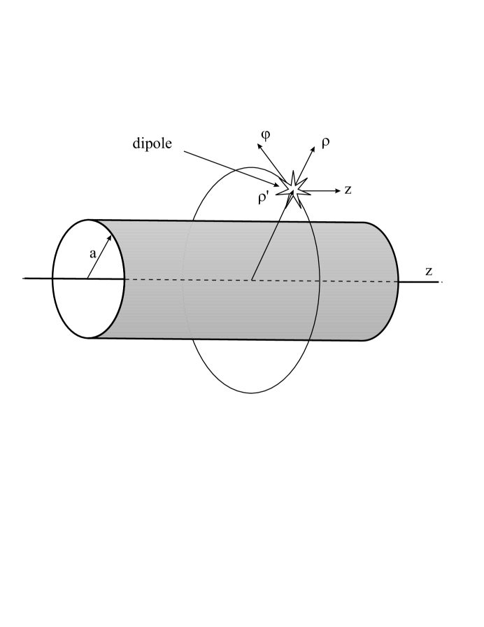
FIG. 1.: Geometry of the problem.

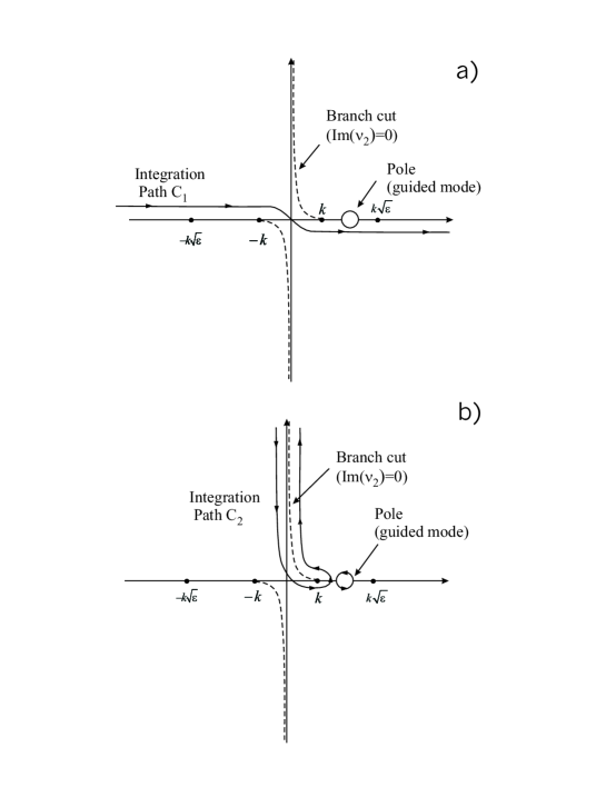
FIG. 2.: Integration path for contour integral over longitudinal wavenumber $h$.

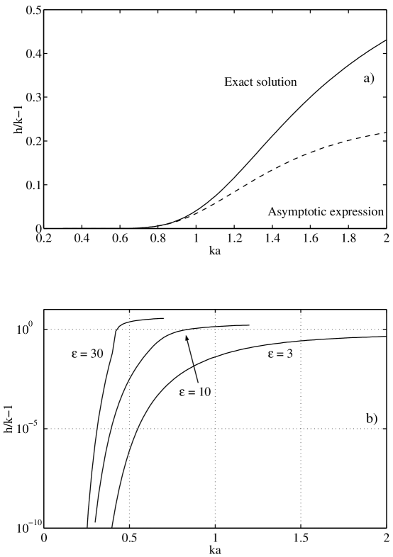
FIG. 3.: Dependence of longitudinal wavenuber of main mode $(h/k)_{01}$ on radius of fiber. a)exact and asymptotic solutions for $\epsilon=3$, b)exact solutions for $\epsilon=3,10,30$.

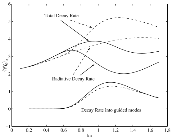
FIG. 4.: Relative decay rates of an atom with $\rho$ orientation as a function of radius of fiber $ka$ [Eq.(65), solid lines]) and its asymptotic expression [Eq.(67), dashed lines]. (atom on the surface, $\varepsilon=3$)

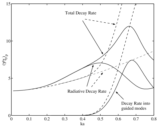
FIG. 5.: Relative decay rates of an atom with $\rho$ orientation as a function of radius of fiber $ka$ [Eq.(65), solid lines]) and its asymptotic expression [Eq.(67), dashed lines]. (atom on the surface, $\varepsilon=10$)

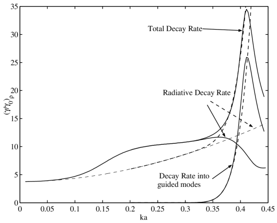
FIG. 6.: Relative decay rates of an atom with $\rho$ orientation as a function of radius of fiber $ka$ [Eq.(65), solid lines]) and its asymptotic expression [Eq.(67), dashed lines]. (atom on the surface, $\varepsilon=30$)

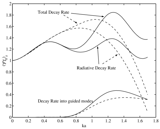
FIG. 7.: Relative decay rates of an atom with $z$ orientation as a function of radius of fiber $ka$ [Eq.(59), solid lines]) and its asymptotic expression [Eq.(60), dashed lines]. (atom on the surface, $\varepsilon=3$)

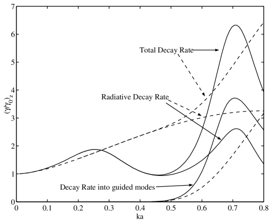
FIG. 8.: Relative decay rates of an atom with $z$ orientation as a function of radius of fiber $ka$ [Eq.(59), solid lines]) and its asymptotic expression [Eq.(60), dashed lines]. (atom on the surface, $\varepsilon=10$)

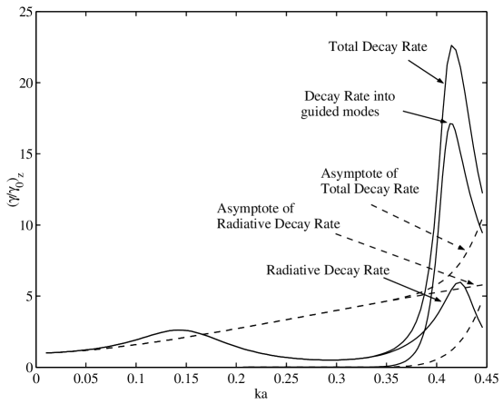
FIG. 9.: Relative decay rates of an atom with $z$ orientation as a function of radius of fiber $ka$ [Eq.(59), solid lines]) and its asymptotic expression [Eq.(60), dashed lines]. (atom on the surface, $\varepsilon=30$)

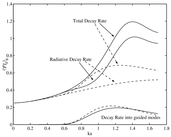
FIG. 10.: Relative decay rates of an atom with $\varphi$ orientation as a function of radius of fiber $ka$ [Eq.(63), solid lines]) and its asymptotic expression [Eq.(64), dashed lines]. (atom on the surface, $\varepsilon=3$)

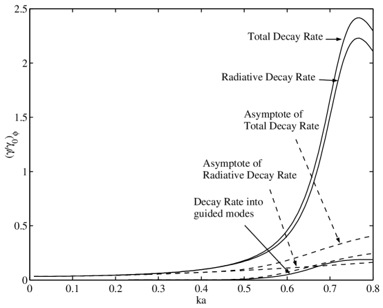
FIG. 11.: Relative decay rates of an atom with $\varphi$ orientation as a function of radius of fiber $ka$ [Eq.(63), solid lines]) and its asymptotic expression [Eq.(64), dashed lines]. (atom on the surface, $\varepsilon=10$)

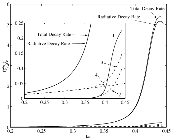
FIG. 12.: Relative decay rates of an atom with $\varphi$ orientation as a function of radius of fiber $ka$ [Eq.(63), solid lines]) and its asymptotic expression [Eq.(64), dashed lines]. (atom on the surface, $\varepsilon=30$). On the inset: 1 - decay rate into guided modes, 2 - asymptotic expression of decay rate into guided modes, 3 - asymptotic expression of total decay rate, 4 - asymptotic expression of radiative decay rate

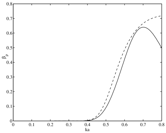
FIG. 13.: The spontaneous emission coupling efficiency [Eq.(71)] as a function of radius of fiber ka (solid lines ) and it asymptotic expressions (dashed lines) ($\rho$ - orientation, $\varepsilon=10$ )

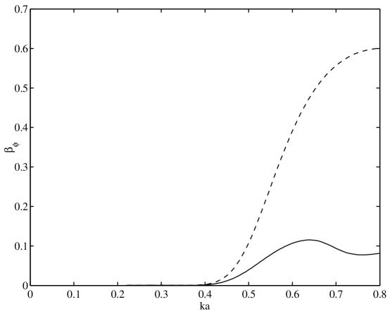
FIG. 14.: The spontaneous emission coupling efficiency [Eq.(71)] as a function of radius of fiber ka (solid lines ) and it asymptotic expressions (dashed lines) ( $\varphi$ - orientation, $\varepsilon=10$ ).

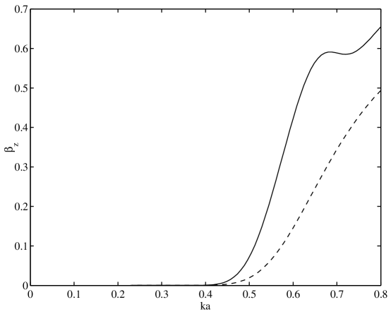
FIG. 15.: The spontaneous emission coupling efficiency [Eq.(71)] as a function of radius of fiber ka (solid lines ) and it asymptotic expressions (dashed lines) (z - orientation, $\varepsilon=10$ ).

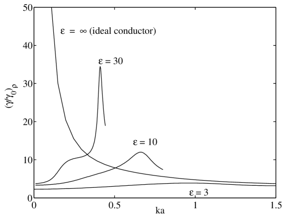
FIG. 16.: Relative linewidth [Eq.(65)] of dipole transitions with $\rho$ orientation as a function of fiber radius ka for different $\varepsilon=3,10,30$ and for ideally conducting cylinder (atom on the surface).

REFERENCES

- [1] E.M. Purcell , Phys. Rev. 69, 681 (1946).
- [2] Cavity Quantum Electrodynamics, edited by P.Berman, (Academic,New York,1994).
- [3] Zh.I. Alferov , Nobel Lecture (2000).
- [4] W.Lucosz, R.E.Kunz, Opt.Comm. 20, 195 (1977).
- [5] G.Barton, J. Phys. B16, 2134 (1974).
- [6] M.Babiker, G.Barton, J. Phys. A9, 129 (1976).
- [7] G. Barton, Proc.R.Soc. Lond. A453, 2461(1997).
- [8] M.Fichet, F.Schuller, D.Bloch, and M.Ducloy, Phys. Rev. A51, 1533, (1995)
- [9] M.-P.Gorza, S.Saltiel, H.Failache and M.Ducloy. The European Physical Journal D15, 113( 2001).
- [10] H.Nha, W.Jhe, Phys.Rev. A 54, 3505 (1996).
- [11] J. Denschlag, G. Umshaus , J. Schmiedmayer , Phys. Rev. Lett. 81, 737(1998).
- [12] J. Denschlag, D.Cassetari , A. Chenet , S. Schneider , J. Schmiedmayer, Appl. Phys. B69 , 291(1999) .
- [13] W.A. Lyon, S.M. Nie, Anal. Chem. 69, 3400 (1997).
- [14] C. Zander, K.H. Drexhage, K.T. Han, J. Wolfrum, M. Sauer, Chem. Phys. Lett. 286, 457 (1998).
- [15] D.Y. Chu, S.T. Ho, J. Optical Society of America B10, 381 (1993).
- [16] D.Y. Chu, S.T. Ho, J.P.Zhang and M.K.Chin, Dielectric Photonic Wells and Wires and Spontaneous Emission Coupling Efficiency of Microdisk and Photonic-Wire Semiconductir Lasers, In:Optical Processes in Microcavities, R.K. Chang, A.J. Campillo (eds.), Word Scientific,1996, P.339-389
- [17] C. Dekker, Physics Today, May, P.22 (1999).
- [18] R. Saito, G. Dresselhaus, M.S. Dresselhaus, Physical Properties of Carbon Nanotubes, Imperial College Press, London, 1998.
- [19] S.D.Brorson, H.Yokoyama, E.P.Ippen, IEEE Journ. of Quant. Electronics 26, 1492 (1990).
- [20] S.D.Brorson,P.M.W.Skovgaard, Optical mode density and spontaneous emission in microcavities, In: Optical Processes in Microcavities, R.K. Chang, A.J.Campillo (eds.), Word Scientific,1996,P.339-389
- [21] M.A. Rippin, P.L. Knight, Journ. Mod. Optics 43, 807 (1996).
- [22] V.V. Klimov, M.Ducloy , Phys. Rev. A62, 043818 (2000).
- [23] B.Z. Katsenelenbaum , Zhurnal Tekhnitcheskoi fiziki XIX, 1168(1949) (In Russian).
- [24] B.Z. Katsenelenbaum , Zhurnal Tekhnitcheskoi fiziki XIX, 1182(1949) (In Russian).
- [25] H. Nha, W. Jhe, Phys.Rev.A56, 2213 (1997).
- [26] J. Enderlein , Chem. Phys.Lett. 301, 430 (1999).
- [27] W. Zakowicz, M.Janowicz , Phys. Rev. A62, 013820 (2000).
- [28] T. Søndergaard and B. Tromborg , Phys. Rev. A64, 033812 ( 2001).
- [29] S.A.Maksimenko, G.Ya.Slepyan, Radiotekhnika i Electronika, 47, 261 (2002) (In Russian)
- [30] I.V.Bondarev, S.A.Maksimenko, G.Ya.Slepyan, Phys.Rev.Lett.,89, 115504 (2002).
- [31] J.D. Jackson, Classical electrodynamics (Wiley, New York, 1975).
- [32] E. Fermi, Rev. Mod. Phys. 4, 87 (1932).
- [33] R.R. Chance, A. Prock, R. Sylbey, Adv. Chem. Phys. 37, 1 (1978).
- [34] J.M. Wylie, J.E. Sipe, Phys. Rev. A30, 1185 (1984); A32, 2030 (1985).
- [35] L. Knöll, S. Scheel, and Dirk-Gunnar Welsch, QED in Dispersing and Absorbing Dielectric Media, Quant-ph/000621-27 June 2000
- [36] Ho Trung Dung, Ludwig Knöll, and Dirk-Gunnar Welsch, Phys. Rev. A64, 013804 (2001)
- [37] A. Tip, L. Knoll, S. Scheel, and D.-G. Welsch , Phys. Rev. A63, 043806 (2001).
- [38] S. Scheel, L. Knoll, and D.-G. Welsch, Phys. Rev. A 58, 700 (1998).
- [39] Ho Trung Dung, L. Knoll, and D.-G. Welsch, Phys. Rev. A 57, 3931 (1998).
- [40] A.F. Stevenson, J. Appl. Phys., 24, 1134 (1953).
- [41] W.R. Smythe, Static and Dynamic Electricity , Third Edition, A SUMMA Book, 1989.
- [42] M. Abramowitz and I.A. Stegun, eds., Handbook of Mathematical Functions (M. NBS, 1964).
- [43] V.V. Klimov, M. Ducloy, and V.S. Letokhov, Kvantovaya Elektronika, 31, 569 (2001).
- [44] V.V. Klimov, M. Ducloy, and V.S. Letokhov, European Physical Journal D20, 133-148 (2002).
- [45] V.V. Klimov, M.Ducloy , Spontaneous emission of single atom placed near metallic nanowires (to be published)
- [46] J.R.Wait, Electromagnetic Radiation from Cylindrical Structures, Pergamon Press, New York,1959.
- [47] G.T. Markov, A.F. Chaplin, Excitation of electromagnetic waves, Moscow, Radio I Svyaz, 1983, 296p. (In Russian).
- [48] B.S.T.Wu , C.Eberlein , Proc. R. Soc. Lond. A455 , 2487 (1998).
- [49] Y.Yamamoto, Coherence, amplification and quantum effects in semiconductor lasers, (John Wiley& Sons, Inc., New York, 1991).