High-order above-threshold ionization: the uniform approximation and the effect of the binding potential

Abstract

A versatile semiclassical approximation for intense laser-atom processes is presented. This uniform approximation is no more complicated than the frequently-used multi-dimensional saddle-point approximation and far superior, since it applies for all energies, both close to as well as away from classical cutoffs. In the latter case, it reduces to the standard saddle-point approximation. The uniform approximation agrees accurately with numerical evaluations for potentials, for which these are feasible, and constitutes a practicable method of calculation in general. The method is applied to the calculation of high-order above-threshold ionization spectra with various binding potentials: Coulomb, Yukawa, and shell potentials which may model C₆₀ molecules or clusters. The shell potentials generate high-order ATI spectra that are more structured and may feature an apparently higher cutoff.

I Introduction

Sufficiently intense laser fields ionize atoms or molecules by the quantum-mechanical process of tunneling DK . Both the tunneling process and the ensuing motion of the electron in the continuum are well accessible to semiclassical methods. Tunneling generates a wave packet whose center follows a classical trajectory while the wave packet is spreading. It may or may not return to within the range of the ionic binding potential. If it does, the well-known recollision-induced processes, such as high-order harmonic generation (HHG) or high-order above-threshold ionization (ATI), take place corkum93 ; MA .

In the tunneling regime, the quantum-mechanical transition amplitude can be analyzed, computed, and interpreted via the saddle-point approximation lew94 ; lew95 . Typically, the transition amplitude is represented by a multi-dimensional integral over the time $t^{\prime}$ at which the electron enters the continuum by tunneling, the later time $t$ at which it revisits the ion, and one or all components of the drift momentum $\mathbf{k}$ along its orbit in between those two times. For a specified final state, e.g., for given final momentum of the electron after the recollision or for given frequency of high-order harmonic emission, the saddle-point approximation selects those particular “quantum orbits” that contribute to this final state. These orbits are characterized by particular values of the parameters $t,t^{\prime}$ and $\mathbf{k}$, which are complex numbers because of the tunneling nature of these orbits. For a specified final state, there are, in general, several contributing quantum orbits. Their contributions have to be added coherently, and this yields an interference pattern, which may appear very intricate, even though its physical origin is simple optcomm ; science .

Within the context of atoms in strong fields, the contributing quantum orbits typically come in pairs. This may be best known from the Lewenstein model of HHG: For specified harmonic order within the “plateau”, there are two quantum orbits whose contributions dominate the harmonic yield, the “long orbit” and the “short orbit”. An electron on the long orbit starts earlier (by ionization) and returns later (for recombination) than an electron on the short orbit lew94 . This is a very general feature of intense-laser–atom processes and holds also for the more complicated orbits, which bypass the ion once or several times before the recombination process takes place optcomm . For fixed laser intensity, the maximal HHG frequency or the maximal energy of an ATI electron obey classical limits corkum93 ; kulander , which are related to the maximal kinetic energy of the electron returning to the ion. For parameters approaching such classical limits, the two quantum orbits become more and more identical. If it were not for the fact that their parameters are complex, reflecting the birth of the electron by tunneling, the two orbits of a pair would coalesce at the classical cutoff optcomm .

The near coalescence of the orbits of a pair near a cutoff constitutes two problems for the saddle-point approximation: (i) treating the two saddle points as independent becomes an increasingly inaccurate approximation if they approach each other closely goresl ; GP00 ; should they actually merge into one, the standard saddle-point approximation diverges and hence is completely inapplicable; (ii) beyond the cutoff, in the classically forbidden regime, both (complex) saddle points continue to exist as formal solutions of the saddle-point conditions. One, however, has to be dropped from the transition amplitude, which is frequently, but not always, indicated by an exponentially exploding contribution. A rigorous analysis establishes that, actually, it is not possible to deform the contour of integration through such a saddle point by the method of steepest descent. In the framework of the theory of asymptotic expansions, the global bifurcation of the steepest-descent contour from two visited saddles to a single visited saddle is known as the Stokes transition BH ; Berry . In previous work, these problems were not treated in a systematic fashion. In this paper, we invoke a specific uniform approximation to solve both problems Henning1 . This turns out to be no more complicated than the standard procedure of treating the two saddle points as independent, because it uses exactly the same information as the standard procedure, namely, the values of the action and its second derivative at the saddle points. Problem (i) is solved because the uniform approximation regularizes the saddle-point integrals close to the classical cutoff, while it reduces to the saddle-point approximation far away from the cutoff. Problem (ii) is solved by imposing the simple requirement of continuity on the transition amplitude, which automatically selects the appropriate branch of the multivalued solution that does not contain the contribution of the unphysical saddle point beyond the classical cutoff. For a zero-range binding potential, the benefit of the saddle-point approximation lies in the insight gained by the introduction of a few quantum orbits, which allow one to visualize the physical mechanism behind recollision-induced processes. For the mere purpose of computation, the transition amplitude can be calculated as well, if not more easily, via a simple quadrature. We will use the zero-range potential as a test case, and find excellent agreement for the uniform approximation, even where the usual saddle-point approximation fails.

The zero-range potential is a valid model for the description of a negatively charged ion in an intense laser field 0range ; manakov ; helm . To what extent it can also be employed to model an atom in an intense laser field or, in other words, just how important the long range of the Coulomb potential is in this situation, has been the object of some debate. Surprisingly, it has turned out that at least for the qualitative explanation of most intense-field effects the Coulomb tail is not instrumental lew94 ; lew95 ; aamop02 . Still more surprisingly, even the subtle quantum-mechanical enhancements of the ATI plateau at certain sharply defined intensities ccres are not specific to the Coulomb potential. In fact, a zero-range potential yields virtually the same enhancements, though at slightly different intensities 0rangeres .

From this point of view, being able to compare ATI spectra from zero-range and non-zero-range potentials is important. However, for non-zero-range potentials, a direct computation of the transition amplitude requires one to carry out a cumbersome multidimensional integral, and the uniform saddle-point approximation is the only viable approach.

The purpose of this paper then is twofold. First, we determine the specific uniform approximation that applies to the pairs of quantum orbits that appear in laser-induced rescattering processes. Second, we use this uniform approximation to investigate the influence of the form of the binding potential on ATI.

The plan of the paper is as follows: In Sec. II, we summarize the improved Keldysh approximation for the transition amplitude. In Sec. III, we discuss the saddle points that feature in the saddle-point approximation as well as in the uniform approximation, and review the saddle-point approximation as well as its problems close to classical cutoffs. In Sec. IV, we determine the uniform approximation that overcomes these problems and describe its conceptual relation to the saddle-point approximation. In Sec. V we compare the ATI spectra obtained by these approximations to the numerical results for the zero-range binding potential. The uniform approximation is then used in Sec. VI to address the effect of a general (non-zero-range) binding potential on the ATI spectrum, using Coulomb, Yukawa, and shell potentials as examples. A summary of the results and conclusions can be found in Sec. VII.

We use atomic units (a.u.) throughout this paper.

II Transition amplitude for rescattering processes

Strong-field phenomena, such as above-threshold ionization (ATI), are successfully described by transition amplitudes derived within a framework known as the strong-field approximation. This approximation neglects the binding potential in the propagation of the electron in the continuum, and the laser field when the electron is bound, which corresponds to treating the process of rescattering in the first-order Born approximation on the background of the laser field. (The first-order Born approximation yields the exact differential cross section in the absence of the field both for the Coulomb potential as well as for the zero-range potential.) The ATI transition amplitude for the direct electrons – electrons that leave the vicinity of the ion right after they have tunneled into the continuum – is the well-known Keldysh-Faisal-Reiss (KFR) amplitude KFR

$$M_{\mathrm{dir}}=-i\int_{-\infty}^{\infty}dt^{\prime}\,\langle\psi_{\mathbf{p}}^{(V)}(t^{\prime})|V|\psi_{0}(t^{\prime})\rangle.$$ (1)

The generalized transition amplitude, which includes one single act of rescattering, is given by LKKB

$$M_{\mathrm{resc}}=-\int_{-\infty}^{\infty}dt\int_{-\infty}^{t}dt^{\prime}\,\langle\psi_{\mathbf{p}}^{(V)}(t)|VU^{(V)}(t,t^{\prime})V|\psi_{0}(t^{\prime})\rangle.$$ (2)

In both equations, $V$ denotes the atomic binding potential, the final state is the Volkov state describing a charged particle with asymptotic momentum $\mathbf{p}$ in the presence of a field with vector potential $\mathbf{A}(t)$,

$$\langle\mathbf{r}|\psi_{\mathbf{p}}^{(V)}(t)\rangle=\exp\left(-\frac{i}{2}\int_{t}^{\infty}d\tau\,[\mathbf{p}+\mathbf{A}(\tau)]^{2}\right)e^{i[\mathbf{p}+\mathbf{A}(t)]\cdot\mathbf{r}},$$ (3)

and $U^{(V)}(t,t^{\prime})$ is the Volkov time-evolution operator, which describes the evolution of the electron in the presence of only the laser field. In Eq. (1), the electron, initially in the ground state $|\psi_{0}(t^{\prime})\rangle$, is ionized into its final state at the time $t^{\prime}$. In Eq. (2), an additional rescattering off the binding potential at the time $t$ is accounted for. The amplitude (2) incorporates the amplitude (1) for direct ionization in the limit where $t^{\prime}\rightarrow t$. Hence, the two amplitudes must not be added LKKB . The amplitude (2) or closely related versions thereof have been used by several authors milos ; goresl ; GP00 ; goresl2 .

If we insert the expansion of the Volkov propagator in terms of Volkov states,

$$U^{(V)}(t,t^{\prime})=\int d^{3}\mathbf{k}\,|\psi_{\mathbf{k}}^{(V)}(t)\rangle\langle\psi_{\mathbf{k}}^{(V)}(t^{\prime})|,$$ (4)

into Eqs. (1) and (2), the transition amplitudes can be rewritten as

$$M_{\mathrm{dir}}=-i\int_{-\infty}^{\infty}dt^{\prime}\,\exp[iS_{\mathbf{p}}(t^{\prime})]\,V_{\mathbf{p}0},$$ (5)

and

$$M_{\mathrm{resc}}=-\int_{-\infty}^{\infty}dt\int_{-\infty}^{t}dt^{\prime}\int d^{3}\mathbf{k}\,e^{iS_{\mathbf{p}}(t,t^{\prime},\mathbf{k})}V_{\mathbf{p}\mathbf{k}}V_{\mathbf{k}0},$$ (6)

where the corresponding actions are given by

$$S_{\mathbf{p}}(t^{\prime})=-\frac{1}{2}\int_{t^{\prime}}^{\infty}d\tau\,\left[\mathbf{p}+\mathbf{A}(\tau)\right]^{2}+|E_{0}|t$$ (7)

and

$$S_{\mathbf{p}}(t,t^{\prime},\mathbf{k}) = -\frac{1}{2}\int_{t}^{\infty}d\tau\,\left[\mathbf{p}+\mathbf{A}(\tau)\right]^{2}$$ (8)

$$- \frac{1}{2}\int_{t^{\prime}}^{t}d\tau\,\left[\mathbf{k}+\mathbf{A}(\tau)\right]^{2}+|E_{0}|t^{\prime}.$$

The quantity $|E_{0}|$ denotes the ionization potential of the atom. In this paper, we address the case of a linearly polarized monochromatic field,

$$\mathbf{A}(t)=A_{0}\mathbf{e}_{x}\cos\omega t,$$ (9)

with the ponderomotive energy $U_{P}=\langle\mathbf{A}^{2}(t)\rangle_{t}/2=A_{0}^{2}/4$.

The representations (5) and (6) are particularly useful if the form factors

$$V_{\mathbf{p}\mathbf{k}} = \left\langle\mathbf{p}+\mathbf{A}(t)\right|V\left|\mathbf{k}+\mathbf{A}(t)\right\rangle$$ (10)

$$= \frac{1}{(2\pi)^{3}}\int d^{3}\mathbf{r}\,\exp[-i(\mathbf{p}-\mathbf{k})\cdot\mathbf{r}]V(\mathbf{r})$$

and

$$V_{\mathbf{k}0} = \left\langle\mathbf{k}+\mathbf{A}(t^{\prime})\right|V\left|0\right\rangle$$

$$= \frac{1}{(2\pi)^{3/2}}\int d^{3}\mathbf{r}\,\exp[-i(\mathbf{k}+\mathbf{A}(t^{\prime}))\cdot\mathbf{r}]V(\mathbf{r})\psi_{0}(\mathbf{r})$$

can be calculated in analytical form. Within the strong-field approximation, the influence of the binding potential is entirely contained in these two matrix elements. For a zero-range potential, the form factors are constants. In this case, the five-dimensional integral (6) can be reduced to a one-dimensional integral over a series of Bessel functions, which can be readily computed numerically LKKB ; JPB . In Sec. V, we will refer to the outcome of this procedure as the “exact result”. In general, however, a correspondingly “exact” evaluation of the matrix element (2) has to deal with a multidimensional integral.

III Saddle-point analysis

For sufficiently high intensity of the laser field, corresponding to small Keldysh parameter $\gamma=\sqrt{|E_{0}|/2U_{P}}$, ionization can be envisioned to proceed via the quasistatic process of tunneling footnkeldysh . The transition amplitudes (5) and (6) are then conveniently computed via the method of steepest descent. Both the standard saddle-point approximation as well as the uniform approximation rest on this method, which approximates the entire integral by the contributions from the vicinity of those points on the integration contour where the action is stationary, i.e., where the partial derivatives of the action with respect to the integration variables vanish. These points correspond to maxima of the integrand after a deformation of the original integration manifold, which is constructed such that the integrand decreases roughly like a Gaussian when one moves away from the vicinity of the saddles BH .

In the current section, we first write down the equations that determine the saddle points, then describe the general procedure of identifying the relevant saddles, and finally discuss the saddle-point approximation. All these items are prerequisites for the discussion of the uniform approximation in Sec. IV.

III.1 Saddle-point equations

For the rescattering amplitude (6), the saddle-point equations are

$$\left[\mathbf{k}+\mathbf{A}(t^{\prime})\right]^{2} = -2|E_{0}|,$$ (12)

$$\left[\mathbf{p}+\mathbf{A}(t)\right]^{2} = \left[\mathbf{k}+\mathbf{A}(t)\right]^{2},$$ (13)

$$\int_{t^{\prime}}^{t}d\tau\left[\mathbf{k}+\mathbf{A}(\tau)\right] = 0.$$ (14)

Their solutions determine the ionization time $t^{\prime}$, the rescattering time $t$, and the drift momentum $\mathbf{k}$ of the electronic orbit in between those two times, such that the electron acquires the asymptotic momentum $\mathbf{p}$. Equations (12) and (13) are related to energy conservation at the ionization time and the rescattering time, respectively, and Eq. (14) determines the intermediate electron momentum. For the direct amplitude (5), only the ionization time $t^{\prime}$ need be determined, and the resulting equation is like Eq. (12) with $\mathbf{k}$ replaced by the asymptotic momentum $\mathbf{p}$.

Evidently, Eq. (12) has no real solutions $t^{\prime}$ as long as $E_{0}\neq 0$, and in consequence $t,t^{\prime}$ and $\mathbf{k}$ are complex. Physically, the fact that $t^{\prime}$ is complex means that ionization takes place through a tunneling process. The solutions $(t,t^{\prime})$ of the saddle-point equations for the linearly polarized monochromatic field (9) have been computed in Ref. optcomm . They only depend on the ionization energy $E_{0}$ and the photoelectron momentum $\mathbf{p}$, but not on the shape of the binding potential, which enters the transition amplitude only via the form factors (10) and (LABEL:ffi).

A very important feature of the solutions is that they come in pairs. Let us denote the “travel time” by $\tau\equiv t-t^{\prime}$. Then, for given asymptotic momentum $\mathbf{p}$ and for the $n$th travel-time time interval $nT/2\leq\textrm{Re}\,\tau\leq(n+1)T/2\ (n=1,2,\dots)$, there are two solutions having slightly different travel times. The parameters of two typical pairs of quantum orbits are displayed in Fig. 1.

III.2 Classical cutoffs and Stokes transitions

The original contour of integration in the amplitudes (5) or (6) is along the real axes, while the solutions of the saddle-point equations (12)–(14) are located off the real axes in the complex plane. A central question in the method of steepest descent then is, which of the various saddle points are visited by the steepest-descent integration manifold. We shall call those the relevant saddle points. The steepest-descent manifold consists of pieces with a constant real part of the action. These pieces are glued together at zeros of the integrand, at which the phase of the action is not well defined. Usually, each piece visits only a single saddle point, which also determines the constant real part of the action. Only such pieces that are needed to connect the integration boundaries give contributions to the transition amplitude. The number of these pieces can change in a so-called Stokes transition, when two pieces merge at a certain value of a parameter (here we consider the photoelectron momentum $\mathbf{p}$). On either side of the Stokes transition, the manifolds of the saddles of interest are glued together in different ways: on one side, both pieces are needed to connect the integration boundaries (plus, possibly, other pieces related to different pairs of saddle points), while only one of the pieces is needed on the other. Note that in the latter case, too, there are still two solutions of the saddle-point equations, but only one of them is visited by the steepest-descent deformation of the original integration manifold kopoldthesis .

Merging of steepest-descent manifolds requires that the real parts of the actions of two quantum orbits become identical at a specific value of $\mathbf{p}$,

$$\mathrm{Re}\,S_{\mathbf{p}}(t_{i},t^{\prime}_{i},\mathbf{k}_{i})=\mathrm{Re}\,S_{\mathbf{p}}(t_{j},t^{\prime}_{j},\mathbf{k}_{j}),$$ (15)

where $i$ and $j$ denote the saddle points of the given pair, and the times $t_{s}$ and $t^{\prime}_{s}\ (s=i,j)$ depend on $\mathbf{p}$. It follows from the physical mechanism behind high-order ATI that both saddles of each pair are relevant provided the asymptotic momentum is classically accessible. For the pair of orbits having the shortest travel times $(n=1)$, this is the case if $\mathbf{p}^{2}/2\leq 10.007U_{P}$ PBW95 . The other pairs of orbits have smaller cutoff energies.

The relevant saddle beyond the classical cutoff is the one that has the smaller imaginary part of the action at the Stokes transition footnote27 . In the following we reserve the index $i$ for this saddle. Saddle $j$ only maintains a residual contribution to the transition amplitude after the Stokes transition, until it becomes completely irrelevant in the so-called anti-Stokes transition

$$\mathrm{Im}\,S_{\mathbf{p}}(t_{i},t^{\prime}_{i},\mathbf{k}_{i})=\mathrm{Im}\,S_{\mathbf{p}}(t_{j},t^{\prime}_{j},\mathbf{k}_{j}).$$ (16)

The anti-Stokes transition coincides with the Stokes transition if both saddles actually coalesce. Otherwise, it frequently occurs very shortly after the Stokes transition.

Exactly how the transition amplitude behaves close to the classical cutoff can only be described when the interplay of both saddles is taken into account in a systematic way, which is achieved by the uniform approximation. Before we turn to this approximation, we now discuss the standard saddle-point approximation.

III.3 Saddle-point approximation

Within the saddle-point approximation, the amplitudes (5) and (6) are approximated by

$$M_{\mathrm{dir}}^{(\mathrm{SPA})}=\sum_{s}\sqrt{\frac{2\pi i}{\partial^{2}S_{\mathbf{p}}/\partial t_{s}^{2}}}V_{\mathbf{p}0}\exp[iS_{\mathbf{p}}(t_{s})]$$ (17)

and

$$M_{\mathrm{resc}}^{(\mathrm{SPA})} = \sum_{s}A_{s}\exp(iS_{s}),$$ (18a)

$$S_{s} = S_{\mathbf{p}}(t_{s},t^{\prime}_{s},\mathbf{k}_{s}),$$ (18b)

$$A_{s} = (2\pi i)^{5/2}\frac{V_{\mathbf{p}\mathbf{k}_{s}}V_{\mathbf{k}_{s}0}}{\sqrt{\det S^{\prime\prime}_{\mathbf{p}}(t,t^{\prime},\mathbf{k})|_{s}}},$$ (18c)

respectively, where the index $s$ runs over the relevant saddle points, and $S^{\prime\prime}_{\mathbf{p}}(t,t^{\prime},\mathbf{k})|_{s}$ is the five-dimensional matrix of the second derivatives of the action (8) evaluated at the solutions of the saddle-point equations (12)-(14).

In explicit calculations, we will proceed slightly differently: First, we employ the saddle-point approximation to evaluate the three-dimensional integral over the intermediate momentum $\mathbf{k}$ in Eq. (6), which enters the action (8) only quadratically. This results in

$$M_{\mathrm{resc}}=-\int_{-\infty}^{\infty}dt\int_{-\infty}^{t}dt^{\prime}e^{iS_{\mathbf{p}}(t,t^{\prime})}V_{\mathbf{p}\mathbf{k}(t,t^{\prime})}V_{\mathbf{k}(t,t^{\prime})0},$$ (19)

where

$$\mathbf{k}(t,t^{\prime})=-\frac{1}{t-t^{\prime}}\int^{t}_{t^{\prime}}d\tau\mathbf{A}(\tau)$$ (20)

and $S_{\mathbf{p}}(t,t^{\prime})\equiv S_{\mathbf{p}}(t,t^{\prime},\mathbf{k}(t,t^{\prime}))$. Then, we again make use of the saddle-point approximation to compute the two-dimensional integral over $t$ and $t^{\prime}$ in Eq. (19), which again results in the amplitude (18), where the actions and amplitudes are now computed by

$$S_{s} = S_{\mathbf{p}}(t_{s},t^{\prime}_{s}),$$ (21a)

$$A_{s} = (2\pi i)^{5/2}\frac{V_{\mathbf{p}\mathbf{k}(t_{s},t^{\prime}_{s})}V_{\mathbf{k}(t_{s},t^{\prime}_{s})0}}{\sqrt{(t_{s}^{\prime}-t_{s})^{3}\det S^{\prime\prime}_{\mathbf{p}}(t,t^{\prime})|_{s}}}.$$ (21b)

The corresponding saddle-point equations are Eqs. (12) and (13) with $\mathbf{k}$ replaced by $\mathbf{k}(t,t^{\prime})$. Note that the values $S_{s}$, $A_{s}$ of each saddle point are not changed, they are just obtained from a different set of relations in this more practical procedure.

Upon approach to the classical cutoff, the two solutions that make up one pair come very close to each other. For an example, this is illustrated in Fig. 1. The saddle-point approximation (18), however, treats different saddle points as independent. As mentioned in previous papers goresl and in the introduction, this leads to a quantitative and qualitative breakdown of the standard saddle-point approximation near the cutoff of any pair of solutions, for two reasons: (i) This approximation can overestimate the contribution to the transition amplitude by several orders of magnitude (it actually diverges if both saddles coalesce). (ii) In previous papers, the spurious saddle has been dropped after the classical cutoff by requiring a minimal discontinuity of the transition amplitude. Still, the discontinuity remains finite and noticeable.

A smooth suppression of the spurious saddle can be achieved if both quantum orbits are well separated at the Stokes transition (which is, however, not the case for physically accessible parameters in ATI), by a regularization that has been derived in the general framework of asymptotic expansions Berry . Thereby, the contribution of the spurious saddle is suppressed by multiplication with the error function

$$\mathrm{erfc}(-\nu)=\frac{2}{\sqrt{\pi}}\int_{-\infty}^{\nu}d\tau\exp(-\tau^{2}),$$ (22)

with the argument given by

$$\nu=\frac{\mathrm{Re}\,[S_{\mathbf{p}}(t_{i},t^{\prime}_{i})-S_{\mathbf{p}}(t_{j},t^{\prime}_{j})]}{\sqrt{2|\mathrm{Im}\,[S_{\mathbf{p}}(t_{i},t^{\prime}_{i})-S_{\mathbf{p}}(t_{j},t^{\prime}_{j})]|}}.$$ (23)

The argument $\nu$ vanishes at the Stokes transition (15) and diverges at the anti-Stokes transition (16), after which the spurious saddle drops out completely. Note that this automatically prevents an exponential growth of the amplitude of the spurious saddle in the approximation (18), because the saddle is dropped while the imaginary part of the action is still positive (namely, equal to the imaginary part of a physical saddle).

This regularization procedure is not accurate enough in the present problem because the Stokes transitions take place while the saddles are not sufficiently separated (cf. Sec. V). On the other hand, the Stokes transitions are already built into the uniform approximation, to which we turn now.

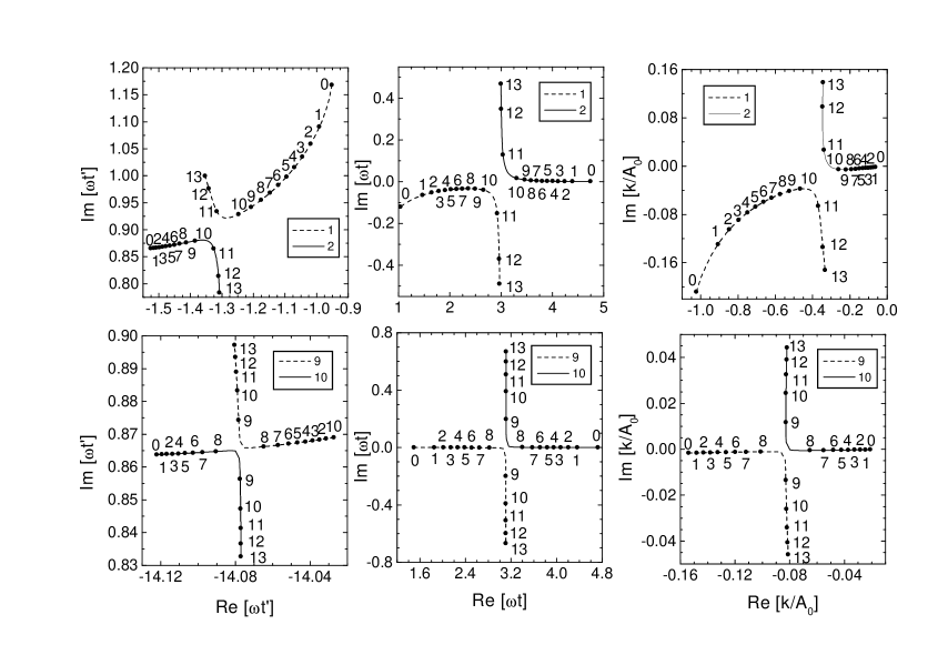
Figure 1: Saddle points as a function of energy for a Keldysh parameter of $\gamma=0.975$ and scattering angle $\theta=0$. The first, second and third column give the start time, the return time, and the intermediate drift momentum, respectively. The panels present the paths in the complex plane that are followed by the saddle points as a function of the final energy, which is indicated by the numbers, which are in multiples of $U_{P}$. The upper row gives the saddle points for the pair of orbits with the shortest two travel times $(1+2)$, the lower row for $(9+10)$, which is one of the pairs with the longest times considered in this paper. The figure shows how the saddle points of a pair approach each other most closely near the classical cutoff. In each case, the contribution of the orbit that is drawn dashed is dropped after the cutoff.

IV The uniform approximation

The saddle-point approximations (17) and (18) are obtained by expanding the action function $S_{\mathbf{p}}$ to second order in the integration variables about each saddle point, and then doing the ensuing Gaussian integrals. These approximations are valid if the expansion of the action holds until the integrand has become much smaller than it was at the saddle point, so that the integration can be extended to infinity. The saddle-point approximation breaks down when the difference of actions $|S_{i}-S_{j}|$ of two quantum orbits with similar coordinates becomes of order unity, such that the expansion about saddle point $i$ becomes inaccurate close to the saddle point $j$, and vice versa. For the quantum orbits in ATI this happens when the energy approaches the classical cutoff. The remedy offered by the theory of asymptotic expansions is to improve the expansion of the action function in the neighborhood of saddles $i$ and $j$ by including higher orders in the coordinate dependence and to take the resulting approximate integral as a collective contribution of both saddle points.

What is often not observed is that the resulting uniform approximation can be written in such a form that no additional information on the quantum orbits is needed, i.e., the cumbersome expansion in the coordinate dependence actually can be circumvented. The derivation proceeds in two steps. First, we write down the so-called diffraction integral which describes a pair of orbits which might be close to each other or well separated. Then, we determine the parameters of the formal expansion in terms of the quantities that enter the standard saddle-point approximation, from the observation that the conventional saddle-point approximation (18) has to be recovered in the limit where the saddle points are sufficiently well separated.

For the first step, we observe that it is precisely two quantum orbits that closely approach each other near each cutoff. According to the splitting lemma of catastrophe theory poston , the parametrization of the integration domain can be rectified such that the orbits approach each other along one of the (appropriately chosen) coordinate axes (denoted by $x$ in the following). This is the only direction where higher orders in the coordinate expansion of the action have to be included, while the expansion in the other coordinates can be restricted to second order such that these can be integrated out by the usual saddle point approximation [this is similar to integrating out $\mathbf{k}$ in the transition from Eq. (18) to Eq. (21)]. Hence the contribution of the pair of quantum orbits (denoted by $i$ and $j$) to the transition amplitude can be reduced, in principle, to a one-dimensional diffraction integral of the general form

$$M_{i+j}=\int_{c_{l}}^{c_{u}}dx\,g(x)\exp[iS(x)],$$ (24)

where the action accounts for these two saddle points and the integration boundaries $c_{u}$, $c_{l}$ in (complex) infinity are assumed such that the integrand decays to zero and the integral converges. Moreover, an expression that reduces to the conventional saddle-point approximation when the quantum orbits are well separated will be obtained if we allow for a linear coordinate dependence in the function $g(x)$. This motivates the use of the normal forms (for a derivation in another semiclassical context, see Ref. Henning1 )

$$S(x)=\bar{S}+\varepsilon x-ax^{3},\qquad g(x)=g_{0}+g_{1}x.$$ (25)

Here we have chosen the origin of the coordinate system exactly in the middle between the two saddles, which have coordinates $x_{i,j}=\pm\sqrt{\varepsilon/3a}$ and coalesce when $\varepsilon=0$.

The uniform approximation that we introduce here differs from an earlier regularization method goresl ; GP00 , where the action was expanded to cubic order about the stationary point corresponding to the classical cutoff. This led to the absence of the linear term in the function $g(x)$ in Eq. (25). It is precisely this term whose presence allows us to match the standard saddle-point approximation both near the cutoff and away from it. Thus, the method of Ref. goresl coincides with the uniform approximation near the classical boundary, but deviates from it and from the exact solution farther away from the cutoff region.

With expansion (25) inserted into the original integral (24), the amplitude $M_{i+j}$ reduces to a sum of Bessel functions,

$$M_{i+j} = \sqrt{2\pi\Delta S/3}\exp(i\bar{S}+i\pi/4)$$

$${}\times\left\{\bar{A}[J_{1/3}(\Delta S)+J_{-1/3}(\Delta S)]\right.$$

$$\left.{}+\Delta A[J_{2/3}(\Delta S)-J_{-2/3}(\Delta S)]\right\},$$

$$\Delta S = (S_{i}-S_{j})/2,\qquad\bar{S}=(S_{i}+S_{j})/2,$$

$$\Delta A = (A_{i}-iA_{j})/2,\quad\bar{A}=(iA_{i}-A_{j})/2,$$

where the four independent parameters $\bar{S}$, $\Delta S=2\varepsilon^{3/2}(27a)^{-1/2}$, $\bar{A}=g_{0}(-2\pi i)^{1/2}a^{1/4}(3\varepsilon)^{-1/4}$, and $\Delta A=g_{1}(2\pi i)^{1/2}\varepsilon^{1/4}(3a)^{-3/4}$ have been expressed by the amplitudes and actions that result from the saddle-point approximation of the diffraction integral (24).

The uniform approximation is defined by inserting into Eq. (LABEL:eq:unif) the actions and amplitudes (18) of the respective pair of quantum orbits (which we denoted by $i$ and $j$). We wish to stress that it is not necessary to obtain the expansion parameters $\bar{S}$, $\varepsilon$, $a$, $g_{0}$, and $g_{1}$ by explicitly carrying out the expansion (25). Indeed, knowledge of the explicit dependence on these parameters is not even desired because it can be manipulated by a coordinate transformation, while the original integral is invariant under smooth changes of the coordinate system. For the saddle-point approximation (18), invariance with respect to coordinate transformations is ensured trivially for the actions $S_{s}$, while the amplitudes $A_{s}$ are invariant because the Jacobian of a transformation contributes a factor to $g$ which is cancelled by the determinant of second derivatives of the action, see Eqs. (18c) and (21b). This is the reason why we express the expansion coefficients in Eq. (25) by the coordinate-transformation invariant quantities $A_{i,j}$, $S_{i,j}$ of the saddle points. Indeed, it is a simple exercise to verify with the help of the asymptotic behavior

$$J_{\pm\nu}(z)\sim\left(\frac{2}{\pi z}\right)^{1/2}\cos(z\mp\nu\pi/2-\pi/4)$$ (27)

of the Bessel functions for large $z$ that the saddle-point approximation (18) is recovered from the uniform approximation (LABEL:eq:unif) in the limit of large $\Delta S$.

Finally, let us demonstrate that the uniform approximation is also capable of describing the Stokes transition, in which one of the two saddles is rendered irrelevant. The Bessel functions in (LABEL:eq:unif) assume complex arguments and are multi-valued functions, depending on the integration contour taken in their integral representation. The functional branches can be distinguished by the number of saddles which are visited by a steepest-descent deformation of the contour, in complete analogy with the procedure for the original integral (6). Hence, when the condition (15) is fulfilled one not only observes a Stokes transition in the original integral, but also encounters a Stokes transition in the defining integral of the Bessel functions. The proper branch of the function will automatically be selected by requiring a smooth functional behavior. The choice of branches beyond the Stokes transition corresponds to replacing the Bessel $J$ functions by Bessel $K$ functions,

$$M_{i+j} = \sqrt{2i\Delta S/\pi}\exp(i\bar{S})$$ (28)

$${}\times\left[\bar{A}K_{1/3}(-i\Delta S)+i\Delta AK_{2/3}(-i\Delta S)\right].\quad$$

From the usual asymptotics

$$K_{\nu}(z)\sim\left(\frac{\pi}{2z}\right)^{1/2}\exp(-z)$$ (29)

of the Bessel $K$ function for large $z$ one verifies that in this case only saddle $i$ contributes to the saddle-point approximation.

In summary, in the uniform approximation the sum of saddle-point amplitudes (18) of each pair of quantum orbits is simply replaced by the collective amplitude (LABEL:eq:unif). The uniform approximation improves the saddle-point approximation such that it works even when two quantum orbits approach each other so closely that one cannot locally expand about either one, as is the case close to their classical cutoff. It also works well far away from classical cutoffs, because it includes the saddle-point approximation as a special case which is recovered for $|\Delta S|\gtrsim 1$. This can happen in two ways: (i) when the saddle points become well separated as a system parameter (such as $\mathbf{p}$) is varied, or (ii) in the strict semiclassical limit when for fixed system parameter the Keldysh parameter is decreased (given $\Delta S\neq 0$). Also, the Stokes transition at the classical cutoff is automatically built into the uniform approximation. Most notably, the uniform approximation is of the same practical simplicity as the saddle-point approximation since it involves the same amplitudes $A_{s}$ and actions $S_{s}$ defined in Eqs. (18).

V Comparing the various approximations

In this section, for the zero-range potential we compare the approximations discussed in the previous sections with the exact integration of Eq. (6). First, let us consider ATI spectra in the direction of the electric field of the laser. Such a spectrum is composed of the contributions of direct and of rescattered electrons. The former quickly decrease after their classical cutoff at $2U_{P}$. The latter form an extended plateau with its classical cutoff at $10U_{P}$, whose yield is below that of the direct electrons by several orders of magnitude. The cutoff at $10U_{P}$ is related to the pair of orbits with the shortest travel times. The other pairs of trajectories, which have longer travel times, have cutoff energies below this value (see, e.g., Ref. optcomm for a more complete discussion). In the figures that follow, we consider up to 5 pairs of electron trajectories, those with the shortest travel times. To each trajectory, we associate a positive integer number which increases with the corresponding travel time.

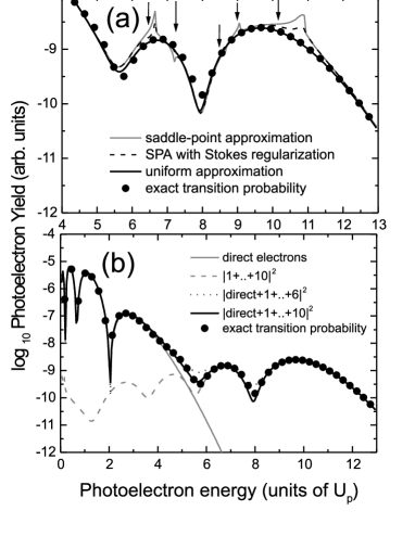
Figure 2: Photoelectron spectra for a zero-range binding potential and $U_{P}/\omega=3.58,$ $\omega=0.073\ {\rm a.u}.,$ and a ground-state energy of $E_{0}=-0.5\ {\rm a.u}.$ The spectrum is in the direction of the electric field of the laser, $\theta=0.$ Part (a) shows spectra computed using the saddle-point and uniform approximations, compared with the photoelectron yield obtained by computing the integral (6) exactly. We take into account the two direct trajectories and five pairs of rescattered trajectories. The approximate energy positions of the Stokes transitions, which coincide with the respective classical cutoffs, are indicated by arrows. Part (b) displays spectra computed by means of the uniform approximation, for direct, rescattered, and both types of electrons, and compares these with the exact integration.

The outcome of this comparison is displayed in Fig. 2(a). In general, there is a good qualitative agreement between the saddle-point approximation and the exact solution (note, however, that the scale is logarithmic in this figure.) Quantitatively, however, there are marked discrepancies, which occur in those energy regions where the saddle points that constitute a particular pair approach each other and can no longer be treated as independent.

In previous work optcomm , the unphysical contribution of one of the saddle points was eliminated by hand as soon as the energy crossed the Stokes line (15). This causes the cusps in the spectra, which can also be seen in Fig. 2(a). This is not very satisfactory, since the discrepancies in the ATI signal may amount to almost one order of magnitude. This problem is particularly critical if the intensity of the driving field is not so high. In this case, the various cutoff energies are relatively close to each other, so that the artifacts affect a broad energy region. Thus, a more accurate approximation is desirable and even necessary, in case the integral (6) cannot be carried out exactly, as is the case for any potential other than the zero-range potential.

One possibility to eliminate such effects, shown in Fig. 2(a), is the Stokes regularization, Eq. (22). This smoothes out the cusps, without, however, eliminating them completely.

Far superior results are obtained by the uniform approximation, given by Eqs. (LABEL:eq:unif) and (28), respectively. The spectrum computed in this way almost perfectly agrees with the exact result. The remaining differences between the uniform approximation and the exact integration occur near the interference minima and are due to the contributions of pairs of trajectories with longer travel times that have not been included. This is indicated by the minor differences in the spectra computed with the uniform approximation using 3 and 5 pairs of trajectories, cf. Fig. 2(b).

Figure 2(b) shows that the exact spectrum is well reproduced by the uniform approximation for all energies. The figure also separately displays the contribution of the direct electrons footdir . One observes that interference between the rescattered and direct electron trajectories is only important within a small energy region, between $4U_{P}$ and $6U_{P}$ Petc00 . Above and below this energy range, either the rescattered or the direct electrons completely dominate the spectrum, so that interference only leads to minor effects.

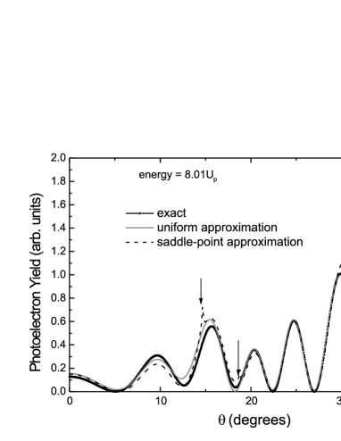
Figure 3: Angular distributions of photoelectrons for the zero-range potential case, computed with the saddle-point and uniform approximations, compared to the exact yield. The field parameters are $U_{P}/\omega=35.8$, $\omega=0.0584\ {\rm a.u}.$, the ground-state energy is chosen as $E_{0}=-0.9\ {\rm a.u}.$, and the photoelectron energy is $\epsilon=8.01U_{P}$. The angles of Stokes transitions are marked with arrows.

The superiority of the uniform approximation over the saddle-point approximation becomes particularly impressive if spectra are displayed on a linear scale. This is done in Fig. 3 for an angular distribution at fixed energy. Both with the saddle-point approximation and the uniform approximation, the 10 shortest trajectories are considered. The uniform approximation, again, yields excellent agreement with the exact result. Minor differences, for small scattering angles, are caused by the trajectories with still longer travel times that have not been included. Those do not contribute for larger angles. The saddle-point approximation, on the other hand, exhibits large discrepancies with the exact results near the classical cutoffs. For the chosen photoelectron energy of $8.01U_{P}$, there are only three relevant cutoffs, corresponding to the pairs of trajectories 1+2, 5+6, and 9+10. The remaining pairs of trajectories do not contribute, since their cutoffs are significantly below $8.01U_{P}$.

VI Influence of the potential on rescattering processes

The preceding section has shown that the uniform approximation is a very dependable method, yielding results very close to those obtained from the exact integration. The latter, however, is only feasible for a binding potential of zero range. Therefore, we will rely on the uniform approximation to investigate how the form of the binding potential affects the photoelectron spectrum. The transition amplitude (2) was derived in the context of one electron bound by the potential $V(\mathbf{r})$. In order to simulate a many-electron atom, it can be reasonable to use in the transition amplitude (2) different potentials $V(\mathbf{r})$ for the electron when it tunnels out and when it rescatters GP00 . In Refs. GP00 ; goresl2 , the effect of the rescattering potential on the general shape of the high-order spectrum and the ratio of direct over rescattered electrons were investigated as a function of the applied field, for the pair of the two shortest orbits. In particular, the dependence on the atomic species was modeled by a Thomas-Fermi potential. Here, for various model potentials, making use of the additional power afforded by the uniform approximation, we will concentrate on the detailed shape of the angular-resolved energy spectrum and on the contributions of the orbits with longer travel times.

Throughout, we shall use the results for the zero-range potential

$$V(r)=\frac{2\pi}{\sqrt{2|E_{0}|}}\delta(\mathbf{r})\frac{\partial}{\partial r}r$$ (30)

as a benchmark. Its form factors (10) and (LABEL:ffi) are constants,

$$V_{\mathbf{p}\mathbf{k}}=\frac{1}{(2\pi)^{2}\sqrt{2|E_{0}|}}$$ (31)

and

$$V_{\mathbf{k}0}=-\frac{(2|E_{0}|)^{1/4}}{2\pi}.$$ (32)

VI.1 Influence of the Coulomb tail

In this subsection, we investigate the influence of the long-range Coulomb potential on above-threshold ionization. This is particularly interesting since for hydrogen ATI spectra have been extracted from a high-precision numerical solution of the time-dependent Schrödinger equation (TDSE) CormLam , so that we can compare the strong-field approximation with an exact solution.

The form factors of the Yukawa potential $V(r)=-Z\exp(-\alpha r)/r$ are

$$V_{\mathbf{p}\mathbf{k}}=-\frac{Z}{2\pi^{2}}\frac{1}{(\mathbf{p}-\mathbf{k})^{2}+\alpha^{2}}$$ (33)

and

$$V_{\mathbf{k}0} = -\frac{\sqrt{2}}{\pi}\frac{Z^{5/2}}{(Z+\alpha)^{2}+[\mathbf{k}+\mathbf{A}(t^{\prime})]^{2}}$$ (34)

$$= -\frac{\sqrt{2}}{\pi}\frac{Z^{5/2}}{(Z+\alpha)^{2}-2|E_{0}|},$$

where the saddle-point equation (12) has been used in the last line. Hence, in the saddle-point approximation, $V_{\mathbf{k}0}$ acts as a constant; indeed, this is the case for any spherically symmetric potential. This constant determines the total ionization rate, but has no effect on the shape of the spectrum. Another consequence is that the spectrum of the direct electrons, described by the amplitude (5), is independent of the form of the binding potential because it only depends on $V_{\mathbf{k}0}$, in contrast to the spectrum of the rescattered electrons.

The Coulomb form factors can be retrieved from Eqs. (33) and (34) in the limit $\alpha\rightarrow 0$. Since in this case $E_{0}=-Z^{2}/2$, this leads to the well-known divergence of the Coulomb form factor (34) lew94 . This has no effect on the shape of the spectrum, and the absolute scale can be reestablished, too rmp .

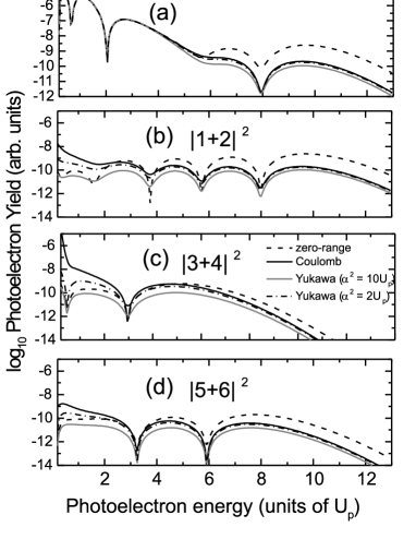
Figure 4: Photoelectron spectra for the zero-range potential, compared with those for the Coulomb and Yukawa potential, for the same field and atomic parameters as in Fig. 2. Panel (a) shows total spectra, while panels (b) to (d) exhibit the contributions of individual pairs of rescattered orbits.

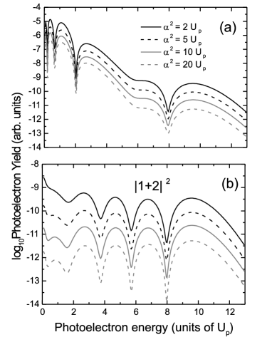
Figure 5: Photoelectron spectra for the Yukawa potential, the same field and atomic parameters as in the previous figure, and several screening parameters $\alpha$. Part (a) shows the resulting spectra for the direct electrons and the five shortest pairs of rescattered orbits, whereas part (b) shows the contributions from the shortest pair of rescattered trajectories.

In Fig. 4, we compare ATI spectra for the zero-range, the Yukawa, and the Coulomb potential. In view of the Coulomb divergence of $V_{\mathbf{k}0}$ we used the zero-range form factor (32) for all potentials footnote2 . As expected from Eq. (33), there is a suppression of the photoelectron yield for the higher energies in the Coulomb and Yukawa cases. This effect is present for all pairs of trajectories. For the Coulomb potential, there is an additional enhancement of the rescattered yield for low energies, which does not occur in the zero-range or short-range cases. This enhancement is due to the functional form of $V_{\mathbf{p}\mathbf{k}}$. Clearly, if the screening parameter is small enough, this effect is also present for the Yukawa potential. Furthermore, for these latter potentials, there is a reduction in the plateau intensity as the screening parameter is increased. Evidently, the form factor (33) for the Coulomb potential always exceeds the one for the Yukawa potential.

The parameters of Figs. 2 and 4 correspond to those chosen in Ref. CormLam , where the results of a numerical solution of the three-dimensional time-dependent Schrödinger equation for hydrogen are reported and ATI spectra are extracted from the former. The agreement between the Coulomb result of Fig. 2 (a) and Fig. 2 of Ref. CormLam is good and even quantitative. We notice that the pronounced dip in the spectrum near $8U_{P}$, which is due to destructive interference of the contributions of the shortest two orbits [cf. Fig. 4 (b)], is almost at the same position in both calculations. The next destructive-interference minimum from these two orbits occurs just below $6U_{P}$. The contributions of the longer orbits [cf. Fig. 4 (c) and (d)] partially fill in this minimum, leaving only a shoulder in the total spectrum (a). The exact calculation CormLam features a slightly more pronounced minimum at the same position. Remarkably, the two interference minima in the total spectrum at low energy near $0.5U_{P}$ and $2U_{P}$, which are due to the direct electrons and the amplitude (5), are also clearly reflected in the exact calculation CormLam at about the same positions. The overall drop of the spectrum from the direct electrons to the final maximum of the rescattered electrons preceding the cutoff is more pronounced in the exact calculation by about half an order of magnitude anotherfootnote .

In Fig. 5, we investigate the ATI spectra for several screening parameters $\alpha$ of the Yukawa potential. In this figure, we also address the question of how the form factor $V_{\mathbf{k}0}$ affects the photoelectron yield. The figure clearly shows a global shift in the photoelectron signal, which increases for decreasing $\alpha$. In this sense, our results are in agreement with those in Ref. milos . It is, however, not expected that this yield increases indefinitely. In fact, its limit for $\alpha\to 0$ should be given by the TDSE results CormLam . Because of the singularity for hydrogen in $V_{\mathbf{k}0}$ for vanishing screening parameters, such a comparison is beyond the scope of the strong-field approximation. Additionally, there is an enhancement of the photoelectron yield at lower energies, similar to those occurring in the Coulomb case, which disappears as $\alpha$ is increased, which is in agreement with the previous figure.

VI.2 Shell potentials

Spherical shell potentials have been used for modeling clusters or molecules such as C₆₀. Recently, ATI has been observed experimentally for C₆₀ in the direct-electron energy region ATIclust . Therefore, in this section we investigate how such potentials affect the ATI spectra in the direct and rescattered regions. Let us first consider a spherical $\delta$-shell,

$$V(r)=-V_{0}\delta(r-r_{0}),$$ (35)

with

$$V_{0}=\frac{\sqrt{2|E_{0}|}}{1-\exp[-2\sqrt{2|E_{0}|}r_{0}]},$$ (36)

where $E_{0}$ again denotes the binding energy of the ground state. Ionization from such a potential was investigated in the past deltashell , for weaker laser fields. The corresponding form factors (10) and (LABEL:ffi) are

$$V_{\mathbf{p}\mathbf{k}}=-\frac{V_{0}r_{0}}{2\pi^{2}\sqrt{(\mathbf{p}-\mathbf{k})^{2}}}\sin[\sqrt{(\mathbf{p}-\mathbf{k})^{2}}r_{0}]$$ (37)

and

$$V_{\mathbf{k}0}=-\frac{V_{0}C}{\pi\sqrt{|E_{0}|}r_{0}}\sinh(\sqrt{2|E_{0}|}r_{0}),$$ (38)

respectively, with

$$C=\left[\frac{\sqrt{2|E_{0}|}}{\exp(2\sqrt{2|E_{0}|}r_{0})-1-2\sqrt{2|E_{0}|}r_{0}}\right]^{1/2}.$$ (39)

For the $\delta$-shell potential, $V_{\mathbf{p}\mathbf{k}}$ is an oscillating function, and $V_{\mathbf{k}0}$ is a constant as always. Thus, in the following, we concentrate on the influence of $V_{\mathbf{p}\mathbf{k}}$ on the resulting spectra. We consider typical C₆₀ parameters, taken from Ref. ATIclust . The external field is chosen such that its intensity is still below the C₆₀ fragmentation threshold, but the electron excursion amplitude footnexcursion is roughly twice as large as $r_{0}$. Furthermore, the Keldysh parameter is about unity. Thus, the rescattering picture is still expected to be applicable.

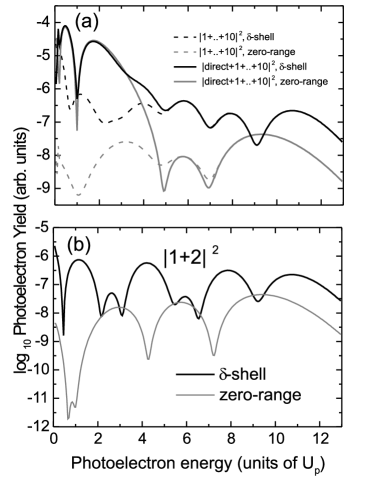
Figure 6: Photoelectron spectra for the shell potential (35), compared with the zero-range case. The ionization potential was taken as $|E_{0}|=0.274$ a.u. and the cluster radius as $r_{0}=6.7$ a.u. The field parameters are $I_{0}=6.5\times 10^{13}\mathrm{W/cm^{2}}$, and $\omega=0.057$ a.u. This yields an excursion amplitude of $a_{0}=13.2$ a.u. and a Keldysh parameter $\gamma=0.9805$. In part (a) we take into account the five shortest pairs of trajectories, whereas in part (b) only the shortest pair is considered.

In Fig. 6, we compare the photoelectron spectrum for the $\delta$-shell and for the zero-range potential, within the uniform approximation. In order to assess the efficiency of rescattering, in either case we used for $V_{\mathbf{k}0}$ the zero-range result (32). The figure shows that the $\delta$-shell potential rescatters more efficiently than the zero-range potential by about one order of magnitude. If the form factor (38) is taken into account, an additional global increase in the yield occurs. However, in the $\delta$-shell case, the rescattering plateau on the average has a downward slope, in contrast to the zero-range case where the slope goes up.

The most interesting feature, however, is that the rescattered spectrum of the $\delta$-shell potential is much more structured than it is for the zero-range potential, with several additional oscillations. Such oscillations are due to the form factor (37), and are already present for the contributions of the shortest pair of trajectories, as shown in Fig. 6(b). An unexpected side effect of these oscillations is the effective increase of the plateau cutoff energy by about two units of $U_{P}$ for the shell versus the zero-range potential, which can be observed in Fig. 6. Since the laser intensity is the same in both cases, the rescattering cutoff would be expected at the same energy, too. However, the shell form factor has a zero around the energy of $9.5U_{P}$, where the zero-range spectrum features its final maximum. This moves the final maximum of the shell-potential spectrum up to a higher energy.

In order to investigate these oscillations in more detail, in the following we will look at contributions of individual trajectories to the photoelectron yield for the $\delta$-shell, in comparison to the zero-range potential. Since the uniform approximation requires pairs of trajectories, we will use the saddle-point approximation for that purpose. Whenever dealing with a pair of trajectories, we will consider the uniform approximation.

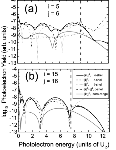
Figure 7: Contribution from individual trajectories to the rescattered photoelectron spectrum for the shell potential, in comparison to the zero-range case. We consider the same parameters as in the previous figure. The labels $i$ and $j$ refer, in part (a), to the third-shortest pair, denoted by (5+6), and in part (b) to the eighth-shortest pair, denoted by (15+16). For the terms $|i+j|^{2}$ we applied the uniform approximation. For the terms $|i|^{2}+|j|^{2}$, we applied the Stokes regularization (22) to the diverging trajectory. The dashed vertical lines in the figure separate the classically allowed and forbidden energy regions for the respective orbits. The dotted and dashed gray lines in part (a) denote the individual contributions of 5 and 6, respectively, for the zero-range case.

Figure 7 displays these results, for several rescattered trajectories. In case $V_{\mathbf{p}\mathbf{k}}$ is constant, as is the case for the zero-range potential, all oscillations present in the spectra come from interference terms. The contributions of individual trajectories are nearly constant in the classically allowed regime and do not produce any substructure. For the $\delta$-shell, however, $V_{\mathbf{p}\mathbf{k}}$ is oscillatory and produces its own maxima and minima in the spectrum. However, comparing Fig. 6(a) and (b) we observe that the contributions of the longer orbits tend to restore the minima of the shell-potential spectrum to those of the zero-range. Only the highest-energy minimum near $9.5U_{P}$ is left unaffected, since the longer orbits do not contribute to this energy.

In particular, the minima are given by $\textrm{Re}\,\sqrt{(\mathbf{p}-\mathbf{k})^{2}}=n\pi/r_{0}$, where $n$ is an integer. To a first approximation, the drift momentum $\mathbf{k}$ can be neglected with respect to the momentum $\mathbf{p}$, so that the energy positions of the minima, in units of the ponderomotive energy, are roughly given by

$$\frac{p^{2}}{2U_{P}}=\frac{n^{2}\pi^{2}}{r_{0}^{2}U_{P}}.$$ (40)

This expression is expected to work better for longer excursion times, since, according to Eq. (14), $\mathbf{k}\propto 1/(t-t^{\prime})$ . This can already be seen in Fig. 1, where the saddle points as functions of the energy are depicted. For a pair of trajectories with short travel times, the start and the return times, as well as the intermediate momentum k, vary considerably with the photoelectron energy. For a long travel time, on the other hand, these quantities are nearly constant, in the classically allowed region. Furthermore, the return time, as well as the intermediate momentum, are almost real and $\mathbf{k}$ is very small.

Clearly, there exist deviations from Eq. (40) due to the fact that $\mathbf{k}$ is non-vanishing and complex, $t$ and $t^{\prime}$ are complex, and due to the time dependence of the intermediate momentum. For instance, a feature that is not explained by Eq. (40) is a shift in the oscillations of the longer trajectory, with respect to those of the short one. This feature occurs for all pairs of trajectories, and decreases as the travel times get longer. A qualitative estimate of these deviations can be obtained by considering $\sqrt{(\mathbf{p}-\mathbf{k})^{2}}$ up to first order in $\sqrt{{\bf k}^{2}}$, and the pair $(t_{1},t_{1}^{\prime})$ and $(t_{2},t_{2}^{\prime})=(t_{1}-\varepsilon,t_{1}^{\prime}+\varepsilon^{\prime})$ up to first order in $\varepsilon,\varepsilon^{\prime}.$ This gives a shift in the minima, which is proportional to $\varepsilon/(t-t^{\prime}),$ confirming the results presented in Fig. 7.

Now we turn to other shell potentials. Similar results are obtained for a more realistic square well, of the form $V(r)=-V_{0}$ for $r_{1}<r<r_{2}$, and zero otherwise. Since, in nature, the sharp edges present for a $\delta$-shell or a square well are smoothed out, it is of interest to investigate whether the additional oscillations are also present for smooth potentials that approximate Eq. (35). One such example is the Gaussian potential

$$V(r)=-V_{0}\exp[-(r-r_{0})^{2}/\sigma^{2}].$$ (41)

For vanishing width, we recover Eq. (35). For this potential, the form factor $V_{\mathbf{p}\mathbf{k}}$ is given by a rather complicated expression, which will not be reproduced here. Important features of $V_{\mathbf{p}\mathbf{k}}$ are the presence of minima and a decrease with increasing asymptotic momentum. This decrease dampens the oscillations, such that $V_{\mathbf{p}\mathbf{k}}$, in comparison to the $\delta$-shell form factor, decays much more rapidly for large $\mathbf{p}$. This effect becomes more pronounced as the width of the potential increases.

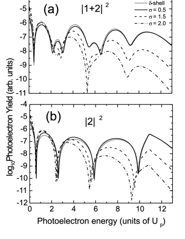
Figure 8: Contribution from the shortest pair of trajectories to the photoelectron spectrum for the Gaussian potential (41), compared to the $\delta$-shell case, for several widths $\sigma$ and the same parameters as in the previous figure. Parts (a) and (b) depict $|1+2|^{2}$ and $|2|^{2}$, respectively. The prefactor $V_{0}$, for $|E_{0}|=0.274$, was computed by solving the time-independent Schrödinger equation numerically.

In Fig. 8(a), the contribution of the two shortest trajectories to the ATI spectra is displayed for the Gaussian potential (41), in comparison to the $\delta$-shell potential. We considered the zero-range-potential form factor $V_{\mathbf{k}0}$ [Eq. (32)]. As in the previous figure, there exist additional oscillations, which come from $V_{\mathbf{p}\mathbf{k}}$. In Fig. 8(b), this is clearly shown, for the contributions from the second shortest trajectory. For small width, as expected, the $\delta$-shell oscillation pattern is practically recovered. For the parameter range considered in the figure, this holds for $\sigma\lesssim 0.5$. Major differences are present only for $\sigma>1.5$. As the width gets larger, there is a displacement in the minima of the form factor and a suppression of the photoelectron yield. This suppression is due to the decay of the form factor $V_{\mathbf{p}\mathbf{k}}$. Therefore, even when the shell potentials are smoothed out, the oscillations survive. Thus, the possibility that they are artificially caused by the sharp edges of the $\delta$-shell potential can be ruled out.

VII Conclusions

We investigate the influence of the binding potential in above-threshold ionization (ATI) for linearly polarized laser fields, in terms of quantum orbits, using the uniform approximation [Eqs. (LABEL:eq:unif) and (28)]. In this method, the transition amplitude is expanded in terms of the collective contribution of pairs of orbits rather than individual orbits. No information is required beyond the conventional saddle-point approximation. This is made possible and, indeed, necessitated by the fact that for laser-induced rescattering phenomena the orbits naturally come in pairs that nearly coalesce at the classical cutoffs, thus rendering the conventional saddle-point approximation inapplicable in this energy region. Moreover, the uniform approximation remains valid beyond the classical cutoff in the classically forbidden region, where it automatically incorporates the fading out of unphysical saddles beyond the cutoff energy. If the two saddles of a pair are sufficiently far apart, the standard saddle-point approximation is recovered.

The fact that the uniform approximation is valid in the whole energy range, both away from as well as near the cutoffs, allows one to obtain quantitative predictions for ATI spectra. Indeed, in this paper this approximation has been tested for the zero-range potential against the numerical computation of the SFA transition amplitudes. The photoelectron spectra, as well as the angular distributions obtained in both ways turned out to be practically identical. With the conventional saddle-point approximation, quantitative predictions are not possible in certain energy regions, which for low laser intensity can span the better part of the ATI plateau.

The excellent quality of the uniform approximation for the zero-range potential also suggests that the uniform approximation is reliable enough for computing ATI spectra for other binding potentials, such as Coulomb, Yukawa, or shell potentials. Within the framework of this paper, the influence of the binding potential is contained in two form factors, which either characterize the transition from the ground state to an intermediate momentum state, or the transition from the intermediate state to an asymptotic momentum state. Throughout the paper, these form factors are called $V_{\mathbf{k}0}$ and $V_{\mathbf{p}\mathbf{k}}$, respectively.

As a first application, we investigated the role of the Coulomb tail by computing photoelectron spectra for Coulomb and Yukawa potentials. As a main feature, we observe a suppression of the photoelectron yield for the ATI plateau, in comparison to the zero-range case, for both Yukawa and Coulomb cases. This is due to the functional forms of $V_{\mathbf{p}\mathbf{k}}$, which are inversely proportional to the photoelectron momentum. Additionally, for the Coulomb potential this form factor causes an increase in the low-energy ATI peaks. These results are in agreement with the fully numerical solution of the time-dependent Schrödinger equation CormLam . Furthermore, for the Yukawa potentials, we observed an increase in the yield for decreasing screening parameter. Similar features have been obtained in milos , from the numerical solution of the strong-field approximation transition amplitudes.

Another class of potentials that we investigated are shell potentials, which are commonly used as an approximation for clusters. In comparison to the zero-range case, the photoelectron spectra computed for such potentials exhibit additional structure, which comes from the oscillating form of $V_{\mathbf{p}\mathbf{k}}$. This is an extreme case of how the form factor $V_{\mathbf{p}\mathbf{k}}$ influences the photoelectron yield. Such oscillations are also present when the potentials are smoothed out, and therefore are not an artifact of the shell models.

An alternative for performing such investigations is the numerical solution of the three-dimensional Schrödinger equation. This would require considerable numerical effort, and, for elliptical polarization, it would take one close to the limit of today’s computational resources. Another possibility would be the numerical solution of the strong-field approximation amplitudes (1) and (2). From the numerical viewpoint, this is not an easy task either, since one must deal with multiple integrals of highly oscillating functions. Thus, the uniform approximation considerably simplifies the computations involved. Furthermore, using this approximation, one is able to gain additional physical insight into the interference processes between the quantum orbits, and how such processes are affected by the binding potential.

Summarizing, the uniform approximation is a very powerful method for investigating laser-assisted rescattering processes, being applicable in all energy regions of the spectra. This approximation allows one to compute photoelectron spectra for binding potentials other than the zero-range with minimal numerical effort. Application of the methods developed in this paper to other high-intensity laser-induced or laser-assisted phenomena, such as non-sequential double ionization, or to elliptically polarized fields is, in principle, straightforward.

- (1) N. B. Delone and V. P. Krainov, Multiphoton Processes in Atoms, (Springer, Berlin, 1994).
- (2) P. B. Corkum, Phys. Rev. Lett. 71, 1994 (1993).
- (3) L. F. DiMauro and P. Agostini, Adv. At., Mol., Opt. Phys. 35, 79 ( 1995).
- (4) M. Lewenstein, Ph. Balcou, M. Yu. Ivanov, A. L’Huillier, and P. B. Corkum, Phys. Rev. A 49, 2117 (1994).
- (5) M. Lewenstein, K. C. Kulander, K. J. Schafer, and P. Bucksbaum, Phys. Rev. A 51, 1495 (1995).
- (6) R. Kopold, W. Becker, and M. Kleber, Opt. Commun. 179, 39 (2000).
- (7) P. Salières, B. Carré, L. Le Déroff, F. Grasbon, G. G. Paulus, H. Walther, R. Kopold, W. Becker, D. B. Milošević, A. Sanpera, and M. Lewenstein, Science 292, 902 (2001).
- (8) K. C. Kulander, K. J. Schafer, and J. L. Krause, in Super-Intense Laser-Atom Physics, Vol. 316 of NATO Advanced Study Institute, Series B: Physics, B. Piraux, A. L’Huillier, and K. Rza̧żewski (editors), (Plenum, New York, 1991), p. 95.
- (9) S. P. Goreslavskii and S. V. Popruzhenko, J. Phys. B 32, L531 (1999); Laser Phys. 10, 583 (2000).
- (10) S. P. Goreslavskii and S. V. Popruzhenko, Zh. Éksp. Teor. Fiz. 117, 895 (2000) [JETP 90, 778 (2000)];
- (11) N. Bleistein and R. A. Handelsman, Asymptotic Expansions of Integrals (Dover, New York, 1986).
- (12) M. V. Berry, Proc. R. Soc. Lond. A 422, 7 (1989).
- (13) H. Schomerus and M. Sieber, J. Phys. A 30, 4537 (1997).
- (14) I. J. Berson, J. Phys. B 8, 3078 (1975); N. L. Manakov and L. P. Rapoport, Zh. Éksp. Teor. Fiz. 69, 842 (1975) [Sov. Phys. JETP 42, 430 (1976)]; F. H. M. Faisal, P. Filipowicz, and K. Rza̧żewski, Phys. Rev. A 41, 6176 (1990); W. Becker, S. Long, and J. K. McIver, Phys. Rev. A 42, 4416 (1990); P. S. Krstić, D. B. Milošević, and R. K. Janev, Phys. Rev. 44, 3089 (1991); G. F. Gribakin and M. Yu. Kuchiev, Phys. Rev. A 55, 3760 (1997).
- (15) B. Borca, M. V. Frolov, N. L. Manakov, and A. F. Starace, Phys. Rev. Lett. 88, 193001 (2002).
- (16) For a recent measurement of the photodetachment spectrum in H-, see R. Reichle. H. Helm, and I. Yu. Kyan, Phys. Rev. Lett. 87, 243001 (2001).
- (17) For a recent review, see W. Becker, F. Grasbon, R. Kopold, D. B. Milošević, G. G. Paulus, and H. Walther, Adv. At., Mol., Opt. Phys., to be published.
- (18) P. Hansch, M. A. Walker, and L. D. Van Woerkom, Phys. Rev. A 55, R2535 (1997); M. P. Hertlein, P. H. Bucksbaum, and H. G. Muller, J. Phys. B 30, L197 (1997); H. G. Muller and F. C. Kooiman, Phys. Rev. Lett. 81, 1207 (1998); H. G. Muller, Phys. Rev. Lett. 83, 3158 (1999); M. J. Nandor, M. A. Walker, L. D. Van Woerkom, and H. G. Muller, Phys. Rev. 60, R1771; E. Cormier, D. Garzella, P. Breger, P. Agostini, P. Chériaux, and C. Leblanc, J. Phys. B 34, L9 (2001).
- (19) G. G. Paulus, F. Grasbon, H. Walther, R. Kopold, and W. Becker, Phys. Rev. A 64, 021401(R) (2001); C. Figueira de Morisson Faria, R. Kopold, W. Becker, and J. M. Rost, Phys. Rev. A 65, 023404 (2002); R. Kopold, W. Becker, M. Kleber, and G. G. Paulus, J. Phys. B 35, 217 (2002).
- (20) L. V. Keldysh, Zh. Éksp. Teor. Fiz. 47, 1945 (1964) [Sov. Phys. JETP 20, 1307 (1965)]; F. H. M. Faisal, J. Phys. B 6, L89 (1993); H. R. Reiss, Phys. Rev. A 22, 1786 (1980).
- (21) A. Lohr, M. Kleber, R. Kopold, and W. Becker, Phys. Rev. A 55, R4003 (1997).
- (22) D. B. Milošević and F. Ehlotzky, Phys. Rev. A 57, 5002 (1998); ibid. 58, 3124 (1998).
- (23) S. P. Goreslavskii and S. V. Popruzhenko, Phys. Lett. A 249, 477 (1998); Pis’ma Zh. Éksp. Teor. Fiz. 68, 858 (1998) [JETP Lett. 68, 902 (1998)].
- (24) R. Kopold and W. Becker, J. Phys. B 32, L419 (1999).
- (25) In practice, the tunneling picture is still applicable if .
- (26) In the case of just one variable, as is the case in the direct amplitude (1), all these statements can be illustrated in straightforward graphical fashion; for an example, see R. Kopold, doctoral dissertation (Technische Universität München, 2001).
- (27) G. G. Paulus, W. Becker, and H. Walther, Phys. Rev. A 52, 4043 (1995).
- (28) Both imaginary parts are positive: As a rule, any saddle that has a negative imaginary part of the action cannot be visited by the steepest-descent contour. This is so because in the original integration the action was real , and the deformation procedure does not lead to an increase of , by construction.
- (29) T. Poston and I. N. Stewart, Catastrophe Theory and its Applications (Pitman, London, 1978).
- (30) Even though the amplitude (2) contains both rescattered and direct electrons, in the context of the saddle-point and the uniform approximation it is preferable to calculate the direct electrons from the amplitude (1) and then, to avoid double counting their contribution, to disregard very short quantum orbits in the amplitude (2); cf. R. Kopold and W. Becker, in Multiphoton Processes, AIP Conference Proceedings No. 525, (American Institute of Physics, Melville, NY, 2000), p. 11.
- (31) For elliptical polarization, the energy range where direct and rescattered electrons interfere is larger, owing to the faster drop of the rescattered electrons for increasing energy. Indeed, interference between direct and rescattered electrons has been observed in this case both in the experiment and in theory; see G. G. Paulus, F. Grasbon, A. Dreischuh, H. Walther, R. Kopold, and W. Becker, Phys. Rev. Lett. 84, 3791 (2000).
- (32) E. Cormier and P. Lambropoulos, J. Phys. B 30, 77 (1997).
- (33) T. Brabec and F. Krausz, Rev. Mod. Phys. 72, 545 (2000).
- (34) Note that, in addition, for the same parameters as in CormLam , the matrix element (34) is singular, such that a direct comparison would not be possible.
- (35) Note that our results include the phase-space factor; that is, all of our spectra plot the quantity .
- (36) E. E. B. Campbell, K. Hansen, K. Hoffmann, G. Korn, M. Tchaplyguine, and M. Wittmann, Phys. Rev. Lett. 84, 2128 (2000).
- (37) G. P. Arrighini, C. Guidotti, and N. Durante, Phys. Rev. A 35, 1528 (1987); S. Patil, Phys. Rev. A 46, 3855 (1992).
- (38) The excursion amplitude is the amplitude of the oscillatory motion of a classical electron in the laser field (9).