Nanometer scale period sinusoidal atom gratings produced by a Stern-Gerlach beam splitter

Abstract

An atom interferometer based on a Stern-Gerlach beam splitter is proposed. Atom scattering from a combination of magnetic quadrupole and homogeneous magnetic fields is considered. Using Raman transitions, atoms are coherently excited into and de-excited from sublevels having nonzero magnetic quantum numbers. The spatial regions in which the atoms are in such sublevels are small and have magnetic fields designed to have constant gradients. Therefore, the atoms experience position-independent accelerations, and the aberration of the coherently separated and recombined atomic beams remains small. We find that because of these properties it is possible to envision an apparatus producing atomic density gratings with nm-scale periods and large contrasts over $10-100$ $\mu$m. We use a new method of describing the atomic interaction with a pulsed spatially homogeneous field. In our detailed analysis, we calculate corrections caused by the non-linear part of the potential and the finite value of the de-Broglie wave length. The chromatic aberration and the effects of an angular beam divergence are analyzed, and optimal conditions for an experimental demonstration of the technique are identified.

I Introduction

An important application of atom interference [1] is the production of a periodic spatial profile of the atomic density. When an atomic beam propagating along the $x$ axis passes through a system of counterpropagating resonant optical fields having wavelength $\lambda$ or through a microfabricated structure having period $\lambda/2$ directed along the $z$ (transverse) axis, an initial atomic state having transverse momentum $p$ splits into a series of states having momenta $p+n\hbar k,$ where $n$ are integers and $k=2\pi/\lambda.$ Interference between these momentum states results in an atomic density pattern, referred to as a grating, having a period $\lambda/2.$ A detailed review and bibliography of the different regimes for producing atomic gratings can be found in our recent article [2].

For the purpose of this paper, it is important to underline that gratings with a sinusoidal density profile and nanometer scale period $\lambda_{g}\ll\lambda,$ say

$$\lambda_{g}\sim 10-100\,nm,$$ (1)

are of particular interest. One method to achieve this goal is to use a large angle beam splitter (LABS), which splits the initial atomic state into two states having momenta $p\pm\Delta p,$ where

$$\Delta p=\pi\hbar/\lambda_{g}.$$ (2)

It was expected that triangular potentials, which one can produce with some accuracy using a strong standing wave field [4], a magneto-optical scheme [5], or bichromatic fields [6], can work as a LABS. However, we recently showed [2, 3] that, asymptotically, the atom density profile scattered from this LABS becomes a spatially inhomogeneous sinusoid with a period of order $\lambda_{g}$ superimposed on sharp density peaks, separated by $\lambda/2.$ The undesired inhomogeneity results from the splitting of the atomic state into two groups of momentum states rather than into two well defined momentum states.

In this article we propose a LABS based on the Stern-Gerlach beam splitter [7, 8]. Our main objective is to test the idea of using this LABS to create sinusoidal atomic gratings with periods much smaller than the optical wavelength but with coherence lengths much larger than the optical wavelength.

The article is arranged as follows. In the next Section, we outline the principles of operation of the proposed devices. In our detailed calculations, we then consider atomic scattering from a finite thickness layer of a linear potential (Section III). Corrections for weak and strong acceleration are evaluated in Sections IV and V. The appendix A is devoted to calculations of the Raman transitions between Zeeman sublevels. We summarize our results in Sec. VI, and discuss their applicability to a beam of ${}^{\text{87}}$Rb atoms.

II Principle of operation

From a naive point of view it seems impossible to use Stern-Gerlach beam splitters for atom interferometry, since such beam splitters produce inerferometer arms corresponding to different Zeeman sublevels. These arms could not interfere. This problem can be avoided as follows (see Fig. 1)

FIG. 1.: Principal scheme of the atom interferometer based on the Stern-Gerlach beam-splitter.

In Fig. 1 we show the principle of the atom interferometer of interest. If an atom having angular moment $G=1/2$ is polarized along the $x$ or $y$ axis, then after splitting by the Stern-Gerlach magnet I, the two arms of the interferometer contain atoms in orthogonal but mutually coherent states having Zeeman quantum numbers $m=\pm 1/2$, respectively. Magnets II and III reflect the atomic beams in the two interferometer arms, and recombine them. Before the recombination, the internal state in one arm of the interferometer is flipped by applying an RF-induced or optically induced $\pi$-pulse in a spatially homogeneous magnetic field. All atoms arrive in the recombination region in the same internal state, and interference occurs.

An ideal sinusoidal grating would arise if an incident plane atomic wavefunction is split into two coherent components in a spatially homogeneous magnetic field gradient. Evidently, a realistic Stern-Gerlach magnet, characterized by a number of higher order spatial derivatives of the magnetic field, does not satisfy this requirement. To realize a magnetic field with constant field gradient, we consider the superposition of a homogeneous bias field ${\bf B}_{s}$ directed along $z$ axis and a quadrupole magnetic field produced by four (anti-)parallel currents propagating in the $\pm y$-directions. This combination allows us to realize a small volume around the center of the quadrupole field in which the field gradient is approximately constant, with no zero of the magnetic field being present. Zeroes of the magnetic field need to be avoided in order to prevent non-adiabatic spin flips (Majorana transitions). Since there are no zeroes of $B$, an atom in a magnetic sublevel $m$ with respect to a quantization axis identical to the $B$-field direction adiabatically follows direction changes of the $B$-field along the atom’s trajectory, and will always remain in that sublevel. The bias field also allowed us to generate potential with a dominant linear term and small nonlinear corrections. The potential for the atom’s center-of-mass motion is then given by $V({\bf r})=g\mu_{B}m\left|{\bf B}({\bf r})\right|$. Atoms prepared in the $m=0$ sublevel do not interact with the field at all.

Based on the preceding considerations, we can now outline how we realize Stern-Gerlach beam splitters with small aberration. We assume that the above described combination of $B$-fields produces a region of almost constant field gradient centered at the origin. A plane matter wave in state $m=0$ propagates in the $+x$-direction. The wave is not refracted or diffracted by magnetic-dipole forces while it traverses the fringe fields of the magnets. External coupling fields are applied in a narrow plane located at $x=-d,$ splitting the wave into a coherent superposition of two waves in different (relevant) Zeeman sublevels (e. g. $m=\pm 1),$. The spin components of the wave experience an acceleration $\propto m$, and acquire a differential transverse momentum change $\Delta p.$ A second set of coupling fields in a plane at $x=+d$ return the accelerated atoms into the state $m=0$ and terminate the interaction with the magnetic field. As a result, the system coherently splits an atomic plane wave entering in a single magnetic sublevel into two momentum components exiting in the same magnetic sublevel. aberration effects, i.e. unwanted curvatures in the phase fronts of the outgoing waves, are minimized by the fact that all magnetic acceleration is localized to a small region $-d<x<d$, in which the field is not strongly contaminated with higher-order multipole terms (“fringe fields”).

If the momentum states overlap spatially, an atomic grating will form. The splitting between Zeeman sublevels caused by the external coupling fields determines the momentum space distribution and the properties of the atom grating in the detection plane. The grating phase is determined by the difference between the atomic wave functions phases acquired along the two arms of the interferometer. Owing to the phase sensitivity to the atom velocity and the magnetic field instability, the grating can be washed out, or one has to require that the atomic beam and field characteristics must be beyond the current state-of-art. One has to choose a splitting scheme and interferometer geometry that minimizes this sensitivity. Two types of interferometers are shown in Fig. 2.

FIG. 2.: Schemes to create atomic gratings with (a) asymmetric and (b) symmetric atom interferometers. I, II, and III are beam-splitters, whose possible layout is shown in Fig. 3.

In the triangular interferometer (Fig. 2a) atoms in arms 1 and 2 have different kinetic energy The phase, associated with this difference, the so called Talbot phase, leads to periodic oscillations of the density distribution [9], initially discovered for light [10] and also observed in an atom interferometer [11]. The Talbot phase plays a critical role in time-domain atom interferometry [12], where it has been used for precise recoil frequency measurements [13]. For interferometers in the spatial domain, the Talbot phase degrades the atom grating, and one should prefer a symmetric interferometer (Fig. 2b) that produces no phase difference.

To produce a symmetric interferometer one first has to split an initial atomic state $\left|m=0\right\rangle$ symmetrically between, for example, states $\left|m=\pm 1\right\rangle.$ Co-propagating cross-polarized optical waves can produce two-quantum transitions between Zeeman sublevels via excited state manifold to create ground state interferometers. Our calculations show that a magnetic field in the acceleration zone can lead to a Zeeman splitting $\omega_{Z}$ larger than the inverse interaction time $\tau_{i}$,

$$\omega_{Z}\tau_{i}\gg 1,$$ (3)

and effective coupling occurs only if one superposes two waves at frequencies $\Omega$ and $\Omega+\omega_{Z}$ needed for a two-quantum resonances. Next, the Zeeman splitting is typically comparable with the excited state hyperfine splitting $\omega_{hf}$, so that, rigorously speaking, to obtain two-quantum transition amplitudes one has to know the excited state manifold structure for a given magnetic field. The situation simplifies if the detuning $\Delta$ between the waves’ frequencies and the ground-excited state transition frequency is larger than both the Zeeman and hyperfine splittings, i.e.

$$\left|\Delta\right|\gg\max\left\{\omega_{Z},\omega_{hf}\right\}.$$ (4)

In this case the reduced matrix element of the two-quantum transition is proportional to that arising in the absence of Zeeman and hyperfine splittings. Since alkali ground states have angular moment $J_{G}=1/2$, selection rules allow field absorption and emission processes only where the angular moment projection changes by at most one, and thus the two-quantum reduced matrix elements between ground state levels vanish. As a result, a combination of $\sigma_{+}-\sigma_{-}$ fields produce no transitions. For this reason we assume here that the fields’ frequencies and polarization vectors are chosen as $\left\{\Omega,{\bf\hat{z}}\right\},$ $\left\{\Omega+\omega_{Z},{\bf\hat{x}}\right\}$, while the atomic initial state is $\left|G=1,m=0\right\rangle,$ where $G$ is the total atomic angular moment (see Fig. 3b). In the atomic rest frame traveling waves localized in the thin layer act as a pulse. For $G=1,$ a proper choice of the pulse area allows one to split all atoms symmetrically between Zeeman sublevels $\left|m=\pm 1\right\rangle$ (see appendix A) and start their acceleration.

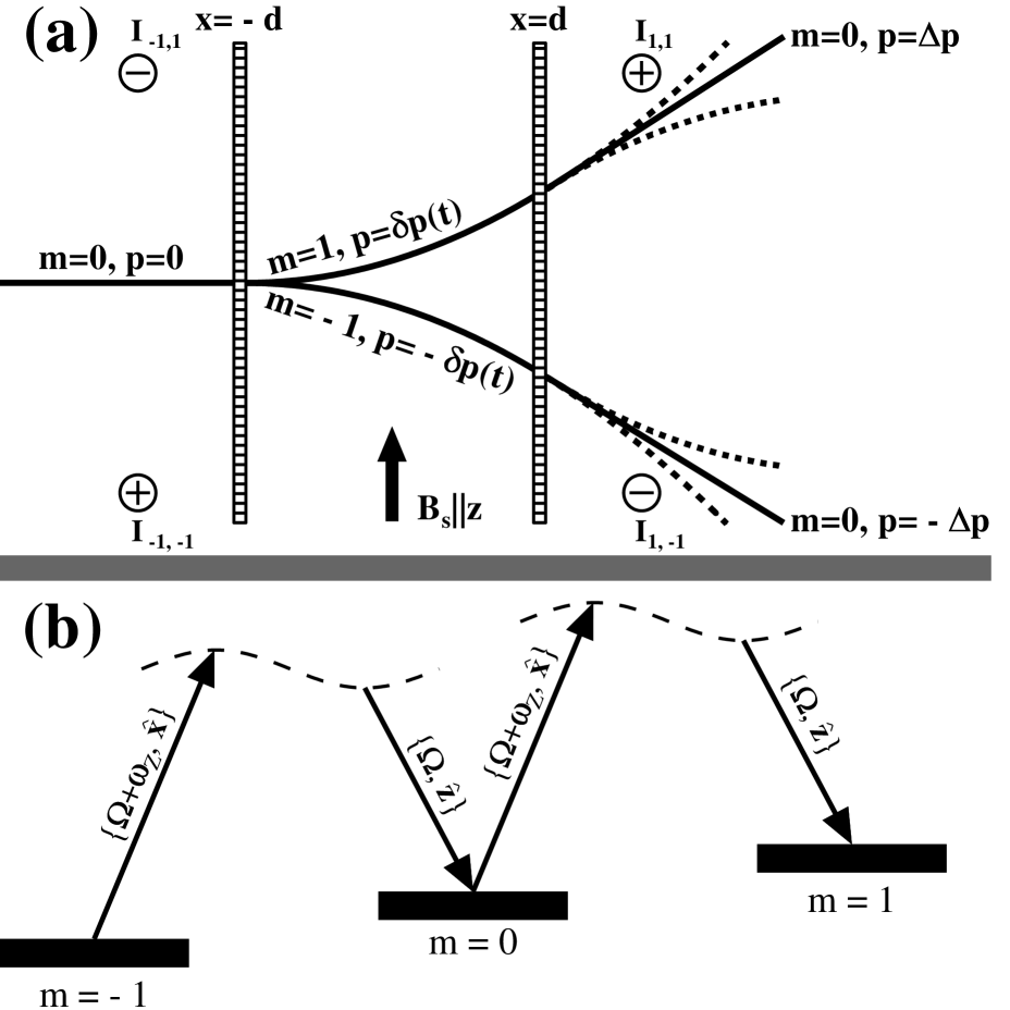
FIG. 3.: (a) Scheme of the beam-splitter. The beam splitter involves four currents $I_{ij}$ comprising a magnetic quadrupole, a homogeneous bias magnetic field ${\bf B}_{s},$ two thin layers of optical fields located at $x=\pm d.$ Initially atoms move without acceleration in the $\left|m=0\right\rangle$ state. In the first layer, atoms split between Zeeman sublevels $\left|m=\pm 1\right\rangle$ and start accelerating. In the second layer atoms are partially returned to the initial state and stop accelerating, while atoms in other sublevels (their trajectories shown by dashed curves) leave the interferometer.                                                                                                              (b) Coupling of the atomic Zeeman sublevels by optical waves propagating along the $y$ axis inside each layer and having frequencies and polarization vectors $\left\{\Omega,{\bf\hat{z}}\right\}$ and $\left\{\Omega+\omega_{Z},{\bf\hat{x}}\right\}$.

To stop the acceleration, one applies another set of traveling waves located on a plane $x=+d$ to return atoms back to the $\left|m=0\right\rangle$ states. The $x$-range within which the acceleration that split the atomic beam are active is thereby limited to the thin region $|x|<d$. One has to distinguish the regimes of weak and strong acceleration, characterized by

$$\eta \ll 1,$$ (6)

$$\eta \gg 1,$$ (7)

respectively, where

$$\eta=\Delta z/b,$$ (8)

$b$ is an atomic beam radius, and $\Delta z$ is the atom displacement during the acceleration. When the acceleration is weak (the case shown in Fig. 3a), on the planes $x=-d$ and $x=+d$ the same pair of fields can be used. Since the Zeeman splitting is equidistant, these fields drive a chain of transitions $\left|m=\pm 1\right\rangle\rightarrow\left|m=0\right\rangle\rightarrow\left|m=\mp 1\right\rangle,$ and, evidently, can not return all atoms to the $\left|m=0\right\rangle$ state. Nevertheless, it is possible to maximize the amplitude of return to the $\left|m=0\right\rangle$ state. At $x>d,$ atoms that remain in the state $\left|m=\pm 1\right\rangle$ continue to accelerate and eventually leave the interferometer, while atoms in the state $\left|m=0\right\rangle$ are of further interest.

In Fig. 2, quadrupoles II and III act along the spatially separated arms of the interferometer, and are adjusted such that they reverse the transverse components of the atomic momenta. For this purpose, one may still apply fields $\left\{\Omega,{\bf\hat{z}}\right\}\$and $\left\{\Omega+\omega_{Z},{\bf\hat{x}}\right\}$ to transfer atoms at $x=-d$ to the states $\left|m=\pm 1\right\rangle,$ decelerate them between $-d<x<d,$ and return them back to the state $\left|m=0\right\rangle$ at $x=+d$. (the origin is assumed to be at the center of the respective quadrupole field). Several additional arms of useless atoms in $\left|m=\pm 1\right\rangle$ states will be produced. Our calculation show that only one-eighth of the atoms will be properly recombined to produce a grating, while seven-eighths will be lost. To avoid the loss, we propose to use a second hyperfine manifold, having angular momentum $G=2.$ If at $x=-d$ one applies fields $\left\{\Omega,{\bf\hat{z}}\right\}\$and $\left\{\Omega+\omega_{21,10},{\bf\hat{x}}\right\},$ where $\omega_{21,10}$ is the frequency of the transition $\left|G=2,m=1\right\rangle\rightarrow\left|G=1,m=0\right\rangle,$ then only this two-level scheme is involved, because the frequencies $n\omega_{21,10}$ ($n\neq 1$ is integer) no longer coincide with any atomic transition frequency. Choosing a field pulse area $\Lambda=\pi,$ one can transfer 100% of the atoms at $x=-d$ into the $\left|G=2,m=1\right\rangle$ state, accelerate the atoms, and return all of them back to the $\left|G=1,m=0\right\rangle$ state at $x=d$ by another $\pi$-pulse.

After the action of quadrupoles I - III of Fig. 2, the total difference of momenta in the interferometer arms is given by

$$\Delta p=\Delta p_{I}+\Delta p_{II}.$$ (9)

Momentum kicks $\Delta p_{i}$ associated with quadrupole $i$ have opposite signs. One needs to use $\Delta p_{II}$ partially to cancel $\Delta p_{I}$. The larger $\left|\Delta p_{II}\right|$ requires a larger field and more severe conditions for the gradient homogeneity. As a result, for a given desirable gratings period $\lambda_{g}$ it is better to choose

$$\left|\Delta p_{I}\right|\ll\left|\Delta p_{II}\right|,$$ (10)

such that

$$\Delta p_{II}\approx\Delta p.$$ (11)

In this case the role of quadrupole I is just to split the beam into two arms, while quadrupoles II and III are responsible almost entirely for the grating formation.

Owing to the inhomogeneity of the field gradient, the finite time of the interaction, and the finite angle of the atom scattering, instead of changing the atom momentum $p$ by fixed value $\Delta p,$ one produces a wave packet in the momentum space near the momentum $p+\Delta p$ with a width that increases for larger momentum kick $\Delta p$ (or smaller $\lambda_{g}).$ We analyzed this effect recently for LABS produced using resonant fields [2, 3]. The atom grating profile would be damaged if the wave packet width becomes larger than $\hbar/b.$ In this article we evaluate corrections to the wave function associated with the factors listed above. For a given grating period $\lambda_{g}$, we find other important characteristics of the problem from the requirement for corrections to be small. These wave function corrections allow us to choose an atomic beam aperture $b$ and velocity $u,$ the length of the interaction zone $d$, the magnetic field gradient $B^{\prime},$ and the bias field strength $B_{s}$ to obtain a desired grating with a given accuracy.

The performance of the various Stern-Gerlach acceleration regions in the above schemes is limited by chromatic aberration and aberrations due to inhomogeneities of the field gradients. The detailed analysis presented in the following sections provides a quantitative foundation to estimate these effects, and to identify the best possible operating conditions.

III Atomic scattering from a linear potential with small corrections

Our Stern-Gerlach beam splitters can be characterized by a potential

$$\tilde{U}\left(z,x\right)=U_{0}\left(x\right)-\tilde{f}\left(x\right)z+\tilde{U}_{1}\left(z,x\right),$$ (12)

which acts on atoms propagating predominantly in the $x$-direction. The potential acts in the narrow layer $\left|x\right|<d$, and consists of a homogeneous part $U_{0}\left(x\right),$ a large linear part $-\tilde{f}\left(x\right)z$, and a small nonlinear addition $\tilde{U}_{1}\left(z,x\right).$ In the following, we analyze the propagation of matter waves in such a potential.

A time-independent solution $\Phi\left(z,x\right)$ of the matter wave at a given energy $E$ in the potential $\tilde{U}\left(z,x\right)$ follows the Schrödinger Equation

$$\left[\frac{{\bf p}^{2}}{2M}+\tilde{U}\left(z,x\right)\right]\Phi\left(z,x\right)=E\Phi\left(z,x\right),$$ (13)

where ${\bf p}$ and $M$ are the momentum operator and the atomic mass. When the potential is weak compared to the kinetic energy, which is mostly given by the motion in $x$-direction,

$$\left|U_{0}\left(x\right)\right|\ll E,$$ (14)

one can use a slowly varying amplitude approximation for the wave function. Introducing a ”time” $t=x/u\left(x\right),$ where

$$u\left(x\right)=\left[2\left(E-U_{0}\left(x\right)\right)/M\right]^{1/2}$$ (15)

is an atomic velocity, one can seek a solution of the form

$$\Phi\left(z,x\right)=\exp\left[i\frac{M}{\hbar}\int_{-d}^{x}dxu\left(x\right)\right]\psi\left(z,t\right),$$ (16)

where $\psi\left(z,t\right)$ is the slowly varying wave function amplitude (referred to below simply as the wave function). In the momentum representation, $\tilde{\Psi}\left(p,t\right)$ =$\left(2\pi\hbar\right)^{-1/2}\int dz\exp\left(-ipz/\hbar\right)\psi\left(z,t\right),$ this wave function obeys the equation

$$i\hbar\partial_{t}\tilde{\Psi}=\left[\frac{p^{2}}{2M}-i\hbar f\left(t\right)\partial_{p}+U_{1}\left(i\hbar\partial_{p},t\right)+Q\right]\tilde{\Psi},$$ (17)

where $f\left(t\right)=\tilde{f}\left(ut\right)$ is a force, $U_{1}\left(z,t\right)=\tilde{U}_{1}\left(z,ut\right),\$and $Q$ represents small terms arising from a second derivative in time and the slow variation of the atomic velocity,

$$Q=-i\frac{\hbar}{2}u^{\prime}\left(x\right)\left(1+i{\displaystyle{\hbar\over Mu^{2}}}\partial_{t}\right)-\frac{\hbar^{2}}{2Mu^{2}}\partial_{t}^{2}.$$ (18)

Neglecting $U_{1}$ and $Q$ one arrives at a one dimensional Schrödinger equation with a time dependent spatially homogeneous force,

$$i\hbar\left(\partial_{t}+f\left(t\right)\partial_{p}\right)\tilde{\Psi}\left(p,t\right)=\frac{p^{2}}{2M}\tilde{\Psi}\left(p,t\right)$$ (19)

Recently, this equation has been exactly solved in the coordinate representation [14, 15, 16]. For the purposes of this article, we derive the solution with an alternate method using the momentum representation and an accelerated frame

$$p = p_{0}+\delta p\left(t\right),$$ (21)

$$\delta p\left(t\right) = \int_{-\tau}^{t}dt_{1}f\left(t_{1}\right),$$ (22)

where the wave function evolves as

$$i\hbar\partial_{t}\tilde{\Psi}\left(p_{0},t\right)=\frac{\left[p_{0}+\delta p\left(t\right)\right]^{2}}{2M}\tilde{\Psi}\left(p_{0},t\right).$$ (23)

Solving this equation and returning back to the lab frame, one finds the following common expression:

$$\tilde{\Psi}\left(p,t\right)=\exp\left[-i\int_{-\tau}^{t}dt_{1}\frac{\left[p+\delta p\left(t_{1}\right)-\delta p\left(t\right)\right]^{2}}{2M\hbar}\right]\tilde{\Psi}\left(p-\delta p\left(t\right),-\tau\right).$$ (24)

If Eq. (17) is written in the accelerated frame (19), the term proportional to $p_{0}^{2}$ is responsible for the matter wave spreading. One can neglect this term if $\tau p_{0}^{2}/2M\hbar\ll 1.$ In the case of a diffraction-limited single-mode atomic beam, $p_{0}$ is a momentum typical of the atomic beam spread, $p_{0}\sim\hbar/b,$ where $b$ is the radius of the incident wave. Then, the just mentioned condition is equivalent to

$$\eta_{1}=\tau/\tau_{s}\ll 1,$$ (25)

where $\tau_{s}=Mb^{2}/\hbar$ is a time characteristic of the spreading of the matter wave. Assuming that this condition is valid we drop the quadratic term in $p_{0}$, and arrive at the equation

$$i\hbar\partial_{t}\tilde{\Psi}\left(p_{0},t\right)=\left[\frac{\delta p^{2}\left(t\right)}{2M}+\frac{\delta p\left(t\right)}{M}p_{0}+U_{1}\left(i\hbar\partial_{p_{0}},t\right)+Q\right]\tilde{\Psi}\left(p_{0},t\right).$$ (26)

Seeking a solution of the form

$$\tilde{\Psi}\left(p_{0},t\right)=\exp\left[-i\phi-ip_{0}\delta z\left(t\right)/\hbar\right]\Psi\left(p_{0},t\right),$$ (27)

where

$$\delta z\left(t\right) = \int_{-\tau}^{t}dt_{1}\frac{\delta p\left(t_{1}\right)}{M},$$ (29)

$$\phi = \int_{-\tau}^{t}dt_{1}\frac{\delta p^{2}\left(t_{1}\right)}{2M\hbar},$$ (30)

one finds that $\Psi\left(p_{0},t\right)$ evolves as

$$i\hbar\dot{\Psi}=\left\{U_{1}\left[\delta z\left(t\right)+i\hbar\partial_{p_{0}},t\right]+Q\right\}\Psi,$$ (31)

where

$$Q = -i\frac{\hbar}{2}u^{\prime}\left(x\right)\left(1+i{\displaystyle{\hbar\over Mu^{2}}}q\right)-\frac{\hbar^{2}}{2Mu^{2}}q^{2},$$ (33)

$$q = \exp\left[i\phi+ip_{0}\delta z\left(t\right)/\hbar\right]\left(\partial_{t}-f\left(t\right)\partial_{p_{0}}\right)\exp\left[-i\phi-ip_{0}\delta z\left(t\right)/\hbar\right].$$ (34)

The wave function in coordinate space at the exit of the interaction zone, $\psi\left(z,\tau\right),$ is given by

$$\psi\left(z,\tau\right)=\exp\left[-i\phi+iz\Delta p/\hbar\right]\int\frac{dp_{0}}{\left(2\pi\hbar\right)^{1/2}}\exp\left[ip_{0}\left(z-\Delta z\right)/\hbar\right]\Psi\left(p_{0},\tau\right),$$ (35)

where

$$\Delta p=\delta p\left(\tau\right)\text{ and }\Delta z=\delta z\left(\tau\right)$$ (36)

is a classical change of the atomic momentum and position under the spatially homogeneous acceleration acting for a time $2\tau.$ One can consider an atomic grating close to sinusoidal, if the period $\lambda_{g}$ is smaller than the transverse extension $b$ of the matter wave, which means that

$$\eta_{2}=\hbar/\Delta pb\ll 1.$$ (37)

In the zeroth order approximation in $U_{1}$ and $Q,$ $\Psi_{0}(p_{0},t)=const$ and, therefore, the zeroth-order wave function (35) is given by the expression

$$\psi_{0}\left(z,\tau\right)=\exp\left[-i\phi+iz\Delta p/\hbar\right]\psi\left(z-\Delta z,-\tau\right),$$ (38)

which can be obtained also from the common solution (24) at the assumption (25). One sees that a matter wave moving with a sufficiently large and time-independent (to neglect term $Q$) velocity $u\$through a layer of the homogeneous force for a time smaller than the packet spreading time is just displaced in the phase space along the classical trajectory.

In the absence of the higher-order effects described below, a purely sinusoidal grating can be formed by interfering atomic momentum components.

IV Weak acceleration

In the following two sections we calculate higher order effects that degrade the ideal scattering behavior of the matter wave.

Consider an atomic beam propagating with velocity $u$ along the $x$-axis and interacting with a quadrupole magnetic field ${\bf B}\left(z,x\right)$ produced by four currents, directed along the $y$-axis, located in the $\left(z,x\right)$ plane at $\left(ia,ja_{x}\right)$ $(i,j=\pm 1),$ and given by $I_{i,j}=Iij.$ In addition to the quadrupole field, one applies a spatially homogeneous magnetic bias field ${\bf B}_{s}={\bf\hat{z}}B_{s},$ such that the total magnetic field is given by

$$B_{z}\left(z,x\right) = -B_{0}\left\{b_{s}+a\sum_{i,j=\pm 1}ij\left(x-ja_{x}\right)\left/\left[\left(z-ia\right)^{2}+\left(x-ja_{x}\right)^{2}\right]\right.\right\},$$ (40)

$$B_{x}\left(z,x\right) = B_{0}a\sum_{i,j=\pm 1}ij\left(z-ia\right)\left/\left[\left(z-ia\right)^{2}+\left(x-ja_{x}\right)^{2}\right]\right.,$$ (41)

where $B_{0}$ is the absolute value of the magnetic field of one current at a distance $a\$and $b_{s}=-B_{s}/B_{0}$. In the rest frame $\left(x=ut\right),$ an atom in the internal state characterized by orbital angular momentum $L_{G},$ electronic spin $S,$ total electronic angular momentum $J_{G},$ nuclear spin $I,$ total angular momentum $G$, and projection $m$ of the total angular momentum on the magnetic field direction, moves in a potential

$$U\left(z,t\right)=\mu\left|{\bf B}\left(z,ut\right)\right|,$$ (42)

where

$$\mu = \left\{1+\left[J_{G}\left(J_{G}+1\right)-L\left(L+1\right)+S\left(S+1\right)\right]/\left[2J_{G}\left(J_{G}+1\right)\right]\right\}$$ (44)

$$\times\left\{\left[G\left(G+1\right)+J_{G}\left(J_{G}+1\right)-I\left(I+1\right)\right]/\left[2G\left(G+1\right)\right]\right\}\mu_{B}m$$

is the projection of the total magnetic moment on the direction of ${\bf B}$, and $\mu_{B}$ the Bohr magneton.

We assume that the atomic beam is centered at $z=0$ and has a radius $b\ll\min\left\{a,a_{x}\right\},$ and that the $\frac{\pi}{2}$- or $\pi$-Raman fields, which turn the interaction with the magnetic field on and off, are located at $x=\pm d$ $\left(d\ll\min\left\{a,a_{x}\right\}\right),$ such that the half-duration of the interaction with the potential (42) is $\tau=d/u.$ When $b_{s}\neq 0,$ one can expand the potential (42) in the vicinity of the $\left(z=0,t=0\right)$ point. Omitting homogeneous term of Eq. 12 and assuming, for simplicity, that there is no explicit time dependence of the force, one finds

$$U\left(z,t\right) = -fz+U_{1}\left(z,t\right),$$ (46)

$$U_{1}\left(z,t\right) = f\sum_{n=2}^{\infty}\sum_{m=0}^{\infty}c_{nm}\left(\alpha,b_{s}\right)\frac{z^{n}}{a^{n-1}}\left(\frac{t}{\tau_{a}}\right)^{2m},$$ (47)

where

$$f=-\mu B^{\prime},$$ (48)

and $B^{\prime}$ is the magnetic field gradient at the quadrupole center, and $\tau_{a}=a/u,$. The dimensionless coefficients

$$c_{nm}\left(\alpha,b_{s}\right)=\frac{a^{n-1}\tau_{a}^{2m}}{fn!\left(2m\right)!}\left.\frac{\partial^{n+2m}U}{\partial z^{n}\partial t^{2m}}\right|_{z=t=0}$$ (49)

depend on the quadrupole size ratio

$$\alpha=a_{x}/a$$ (50)

and the bias field’s relative strength $b_{s}.$ For a magnetic quadrupole, the coefficients $c_{nm},$ used in further calculations, are given by

$$c_{21} = 16\alpha\left[16\alpha^{2}-3b_{s}^{2}\left(\alpha^{2}-1\right)\left(\alpha^{2}+1\right)^{2}\right]b_{s}^{-3}\left(\alpha^{2}+1\right)^{-6},$$ (52)

$$c_{22} = -16\alpha\left[1536\alpha^{4}-352\alpha^{2}b_{s}^{2}\left(\alpha^{2}-1\right)\left(\alpha^{2}+1\right)^{2}+b_{s}^{4}\left(\alpha^{2}+1\right)^{4}\left(21-62\alpha^{2}+21\alpha^{4}\right)\right]b_{s}^{-5}\left(\alpha^{2}+1\right)^{-10},$$ (53)

$$c_{23} = -16\alpha\left\{-122880\alpha^{6}+35328b_{s}^{2}\alpha^{4}\left(\alpha^{2}-1\right)\left(\alpha^{2}+1\right)^{2}-32b_{s}^{4}\alpha^{2}\left(\alpha^{2}+1\right)^{4}\left(95-234\alpha^{2}+95\alpha^{4}\right)\right.$$ (55)

$$+\left.b_{s}^{6}\left(\alpha^{2}+1\right)^{6}\left[81\left(\alpha^{6}-1\right)-463\alpha^{2}\left(\alpha^{2}-1\right)\right]\right\}b_{s}^{-7}\left(\alpha^{2}+1\right)^{-14},$$

$$c_{30} = 2\left(\alpha^{2}-1\right)\left(\alpha^{2}+1\right)^{-2}.$$ ()

To indicate the structure of the $c_{nm}$, in the following matrix indices $\left(n,m\right)$ with $c_{nm}\neq 0$ are marked by a “V”:

$$\left(\begin{tabular}[]{|c|c|c|c|c|}\hline\cr&$m=0$&1&2&3\\ \hline\cr$n=2$&&V&V&V\\ \hline\cr 3&V&V&V&V\\ \hline\cr 4&&V&V&V\\ \hline\cr 5&V&V&V&V\\ \hline\cr\end{tabular}\right).$$ (56)

We characterize the problem by dimensionless parameters

$$\beta = b/a,\,$$ (58)

$$\delta = d/a,\,\,$$ (59)

$$\varepsilon_{g} = \lambda_{g}/a,$$ (60)

$$\theta = \lambda_{dB}/\lambda_{g},$$ (61)

where

$$\lambda_{dB}=2\pi\hbar/Mu$$ (62)

is the atomic de-Broglie wavelength and $\theta$ is the angle of atom scattering. The constant force one needs to apply to achieve a given atomic grating period can be found from Eqs. (36, 19, 2) to be

$$f=\kappa\pi\hbar u/2d\lambda_{g},$$ (63)

where the parameter $\kappa\approx 1$ for quadrupoles $II$ and $III,$ and $\kappa=\Delta p_{I}/\Delta p\ll 1$ for quadrupole $I$ (see Fig. 2b). Consequently, the atom displacement $\Delta z=\kappa d\theta/2$ and the parameter (8) is given by

$$\eta=\kappa\delta\theta/2\beta,$$ (64)

while the small parameters (25, 37) are given by

$$\eta_{1} = \left(2\pi\right)^{-1}\delta\theta\varepsilon_{g}\beta^{-2},$$ (66)

$$\eta_{2} = \varepsilon_{g}/\pi\beta.$$ (67)

One can express the atomic beam and magnetic quadrupole characteristics through the parameters (IV). For example, using Eqs. (61, 62) and then (63, 48, 59), one finds the atom velocity and magnetic field gradient:

$$u = \left(2\pi\hbar/M\lambda_{g}\right)\theta^{-1},$$ (69)

$$B^{\prime} = \left(\kappa\pi^{2}\hbar^{2}/\mu M\lambda_{g}^{3}\right)\varepsilon_{g}\theta^{-1}\delta^{-1}.$$ (70)

One can use Eq. (31) to calculate corrections to the unperturbed atom wave function $\psi_{0}\left(p_{0},t\right)=\psi\left(p_{0},-\tau\right).$ Using the estimate

$$\hbar\partial_{p_{0}}\sim b,$$ (71)

for the case of weak acceleration (6), one can neglect the term $\delta z\left(t\right)$ in Eq. (31). After this, one can calculate the first-order correction $\Psi_{1}(p_{0},\tau),$ associated with the $\left(n,m\right)$ term of the expansion (30). Substituting the expression for $\Psi_{1}(p_{0},\tau)$ in Eq. (35) one finds the correction in the coordinate representation

$$\psi_{1}\left(z,\tau\right)=-i\left[2fc_{nm}d^{2m+1}\right/\left.\left(2m+1\right)\hbar a^{n+2m-1}u\right]\left(z-\Delta z\right)^{n}\psi_{0}\left(z,\tau\right),$$ (72)

where $\psi_{0}\left(z,\tau\right)$ is given by Eq. (38)

We now proceed to calculate the correction $\Psi_{q}(p_{0},\tau)$ associated with a term $Q$ in Eq. (31). In Appendix B we found the conditions under which one can neglect the first term in the Eq. (33), while the operator (34) is reduced to the expression

$$q\approx-f\partial_{p_{0}}.$$ (73)

Consequently, the relevant correction in coordinate space is given by

$$\psi_{q}\left(z,\tau\right)=-i\left(f^{2}\tau/\hbar Mu^{2}\right)\left(z-\Delta z\right)^{2}\psi_{0}\left(z,\tau\right).$$ (74)

In contrast to (72), this correction arises from the wave packet motion through a field with a homogeneous gradient.

The parameters $\beta,$ $\delta$ and $\theta$ have to be chosen such that corrections (72, 74) are small. We estimate these corrections at $z-\Delta z=b.$ Introducing a small parameter

$$\varepsilon_{q}=\left|\psi_{q}\left(\Delta z+b,\tau\right)/\psi\left(\Delta z+b,\tau\right)\right|$$ (75)

one finds for $\theta$

$$\theta=e_{q}\varepsilon_{g}\varepsilon_{q}\delta\beta^{-2},$$ (76)

where

$$e_{q}=8\pi^{-1}\kappa^{-2}$$ (77)

Among the corrections $\psi_{1}$ for different $n$ and $m,$ the leading terms arise from

$$\left(n,m\right) = \left(2,m_{1}\right),$$ (79)

$$\left(n,m\right) = \left(n_{2},0\right),$$ (80)

as they are the first non-zero terms in the row $n=2$ or column $m=0$ of the matrix (56), and the other terms are higher powers of the small parameters $\tau/\tau_{a}=\delta$ or $\left|\left(z-\Delta z\right)/a\right|\lesssim\beta.$ Introducing the corresponding small parameters $\varepsilon_{1}$ and $\varepsilon_{2}$ for the relative weight of corrections related to Eqs. (IV) and using Eq. (72), one arrives at equations

$$\delta^{2m_{1}}\beta^{2} = e_{1}\varepsilon_{g}\varepsilon_{1},$$ (82)

$$\beta^{n_{2}} = e_{2}\varepsilon_{g}\varepsilon_{2},$$ (83)

where

$$e_{1}=\left(2m_{1}+1\right)\left(\kappa\pi\left|c_{2m_{1}}\right|\right)^{-1},\,\,e_{2}=\left(\kappa\pi\left|c_{n_{2}0}\right|\right)^{-1}.$$ (84)

Solving Eqs. (IV) one finds

$$\delta = \varepsilon_{1}^{1/2m_{1}}\varepsilon_{2}^{-1/m_{1}n_{2}}\varepsilon_{g}^{\left(n_{2}-2\right)/2m_{1}n_{2}}f_{\delta}\left(\alpha,b_{s}\right),$$ (86)

$$f_{\delta}\left(\alpha,b_{s}\right) = e_{1}^{1/2m_{1}}e_{2}^{-1/m_{1}n_{2}},$$ (87)

$$\beta = \left(\varepsilon_{g}\varepsilon_{2}\right)^{1/n_{2}}f_{\beta}\left(\alpha,b_{s}\right),$$ (88)

$$f_{\beta}\left(\alpha,b_{s}\right) = e_{2}^{1/n_{2}}$$ (89)

$$\theta = \varepsilon_{1}^{1/2m_{1}}\varepsilon_{2}^{-\left(2m_{1}+1\right)/m_{1}n_{2}}\varepsilon_{q}\varepsilon_{g}^{1+\left(n_{2}-4m_{1}-2\right)/2m_{1}n_{2}}f_{\theta}\left(\alpha,b_{s}\right),$$ (90)

$$f_{\theta}\left(\alpha,b_{s}\right) = e_{1}^{1/2m_{1}}e_{2}^{-\left(2m_{1}+1\right)/m_{1}n_{2}}e_{q}.$$ (91)

One can use Eqs. (IV) to estimate the efficiency of the beam splitter with arbitrary non-linearity.

We now return to the quadrupole configuration at hand. The non-linearities depend on the ratio of the quadrupole sizes $\alpha$ and the relative strength of the bias magnetic field $b_{s}.$ These quantities can be used to diminish the role of the non-linearities. One can choose  them such that either the coefficient $c_{21}$ or the coefficient $c_{30}$ vanishes. Our calculations show that it is more effective to choose $c_{21}=0$; therefore, in the remainder of this article, we consider that case. Equation

$$c_{21}=0$$ (92)

determines the ratio of the size $\alpha$ as a function of $b_{s}.$ The function $\left.\alpha\left(b_{s}\right)\right|_{c_{21}=0}$ is shown in Fig. 4a.

FIG. 4.: Dependence of the quadrupole size ratio $\left(a\right),$ width of the acceleration zone $\left(b\right),$ atomic beam radius $\left(c\right),$ and scattering angle $\left(d\right)$ on the relative strength $b_{s}$ of bias magnetic field.

For $c_{21}=0$ the lowest-order correction is the term corresponding to $m_{1}=2,$ $n_{2}=3$ (see matrix (56)). The functions $f\left[\alpha\left(b_{s}\right),b_{s}\right]$ are plotted in Fig. 4 for $\kappa=1.$ These functions have notable features for the relative field strength $b_{s}\approx 0.537,$ where the ratio of quadrupole size (50) is $\alpha\approx 1.99.$ These singular features arise because at $b_{s}\approx 0.537$ - in addition to condition (92) - the non-linearity that is quadratic in space and 4th-order in time also vanishes, i. e.

$$c_{22}=0.$$ (93)

So, one has to consider the next term, $\left(2,3\right),$ in the row $n=2$ of the Table (56). When $m_{1}=n_{2}=3$ and $\left(\alpha,b_{s}\right)$ is a root of Eqs. (92, 93), one finds from Eqs. (IV):

$$\delta = 1.45\varepsilon_{1}^{1/6}\varepsilon_{2}^{-1/9}\varepsilon_{g}^{1/18},$$ (95)

$$\beta = 0.871\left(\varepsilon_{2}\varepsilon_{g}\right)^{1/3},$$ (96)

$$\theta = 3.19\kappa^{-25/18}\varepsilon_{1}^{1/6}\varepsilon_{2}^{-7/9}\varepsilon_{q}\varepsilon_{g}^{7/18}.$$ (97)

V Strong acceleration.

When $\eta\gg 1,$ one can expand the nonlinear part of the potential $U_{1}$ in Eq. (31) in the operator $i\hbar\partial_{p_{0}}.$ The zeroth-order term $U_{1}\left[\delta z\left(t\right),t\right]$ depends only on time and, therefore, changes the phase of the atomic wave function (27) to the value

$$\phi=\frac{1}{\hbar}\int_{-\tau}^{t}dt_{1}\left[\frac{\delta p^{2}\left(t_{1}\right)}{2M}+U_{1}\left[\delta z\left(t_{1}\right),t_{1}\right]\right].$$ (98)

After a phase transformation one arrives at the equation

$$i\hbar\dot{\Psi}=\left\{U_{z}\left(t\right)i\hbar\partial_{p_{0}}+Q\right\}\Psi,$$ (99)

where

$$U_{z}\left(t\right)=\left.\frac{\partial U_{1}\left(z,t\right)}{\partial z}\right|_{z=\delta z\left(t\right)}.$$ (100)

Since one can still neglect the first term in Eq. (33) and use Eq. (73) for the operator $q$ (see Appendix B), the previously calculated correction $\psi_{q}\left(z,\tau\right),$ associated with the $Q$-term, and, therefore, Eq. (76) are still valid. Using the expansion (47) one obtains a series for the operator (100). Keeping only the $\left(n,m\right)$ term of this series in the right-hand-side of Eq. (99), one finds that the corresponding correction in the coordinate representation is given by

$$\psi_{1}\left(z,t\right)=-i\left[nc_{nm}I_{nm}f^{n}d^{2\left(m+n\right)-1}\left(z-\Delta z\right)/\hbar a^{2m+n-1}u^{2n-1}\left(2M\right)^{n-1}\right]\psi_{0}\left(z,t\right),$$ (101)

where

$$I_{nm}=\int_{-1}^{1}d\xi\xi^{2m}\left(1+\xi\right)^{2\left(n-1\right)}.$$ (102)

Requiring the magnitude of this correction at $z=\Delta z+b$ to be $\varepsilon_{1}$- and $\varepsilon_{2}$-times smaller than the zeroth-order solution $\psi_{0}\left(z,t\right)$ for $\left(n,m\right)=\left(2,m_{1}\right)$ and $\left(n_{2},0\right),$ respectively, and expressing the atom velocity $u$ and the force $f$ through parameters (IV), one obtains equations

$$\beta\delta^{1+2m_{1}}\theta = e_{1}\varepsilon_{g}\varepsilon_{1},$$ (104)

$$\beta\left(\delta\theta\right)^{n_{2}-1} = e_{2}\varepsilon_{g}\varepsilon_{2},$$ (105)

where for this case we define parameters $e_{i}$ as

$$e_{1}=8/\kappa^{2}\pi c_{2m_{1}}I_{2m_{1}},\,\,e_{2}=2^{3n_{2}-2}/\kappa^{n_{2}}\pi n_{2}c_{n_{2}0}I_{n_{2}0}.$$ (106)

Equations (76, 102) constitute a system for three variables $\delta,$ $\beta,$ $\theta,$ which has the solution

$$\delta = \varepsilon_{1}^{\left(2n_{2}-3\right)/2\gamma}\varepsilon_{2}^{-1/2\gamma}\left(\varepsilon_{g}/\varepsilon_{q}\right)^{\left(n_{2}-2\right)/2\gamma}f_{\delta}\left(\alpha,b_{s}\right),$$ (108)

$$f_{\delta}\left(\alpha,b_{s}\right) = e_{1}^{\left(2n_{2}-3\right)/2\gamma}e_{2}^{-1/2\gamma}e_{q}^{-\left(n_{2}-2\right)/2\gamma},$$ (109)

$$\beta = \varepsilon_{1}^{\left(n_{2}-1\right)/\gamma}\varepsilon_{2}^{-\left(m_{1}+1\right)/\gamma}\varepsilon_{g}^{\left(n_{2}-2\right)\left(m_{1}+1\right)/\gamma}\varepsilon_{q}^{m_{1}\left(n_{2}-1\right)/\gamma}f_{\beta}\left(\alpha,b_{s}\right),$$ (110)

$$f_{\beta}\left(\alpha,b_{s}\right) = e_{1}^{\left(n_{2}-1\right)/\gamma}e_{2}^{-\left(m_{1}+1\right)/\gamma}e_{q}^{m_{1}\left(n_{2}-1\right)/\gamma},$$ (111)

$$\theta = \varepsilon_{1}^{-\left(2n_{2}-1\right)/2\gamma}\varepsilon_{2}^{\left(4m_{1}+3\right)/2\gamma}\left(\varepsilon_{g}/\varepsilon_{q}\right)^{\left[2\left(m_{1}+1\right)-n_{2}\right]/2\gamma}f_{\theta}\left(\alpha,b_{s}\right),$$ (112)

$$f_{\theta}\left(\alpha,b_{s}\right) = e_{1}^{-\left(2n_{2}-1\right)/2\gamma}e_{2}^{\left(4m_{1}+3\right)/2\gamma}e_{q}^{-\left[2\left(m_{1}+1\right)-n_{2}\right]/2\gamma}$$ (113)

where $e_{q}$ is defined by Eq. (77) and $\gamma=n_{2}-2+m_{1}\left(2n_{2}-3\right)$.

The further consideration is the same as in the previous Section. If one chooses the quadrupole axes ratio $\alpha$ such that the potential’s quadratic term in space and time vanishes, i.e. if $\alpha\equiv\alpha\left(b_{s}\right),$ where the function $\alpha\left(b_{s}\right)$ is defined explicitly by Eq. (92) and shown in Fig. 4a, then again $m_{1}=2$ and $n_{2}=3.$ The functions $f\left[\alpha\left(b_{s}\right),b_{s}\right]$ are shown in Fig. 5.

FIG. 5.: Strong acceleration regime. Dependences of the width of the acceleration zone $\left(a\right),$ atomic beam radius $\left(b\right),$ and scattering angle $\left(c\right)$ on the bias magnetic field relative strength $b_{s}$.

At the point of divergence, $b_{s}\approx 0.537,$ choosing $m_{1}=n_{2}=3,$ one finds

$$\delta = 1.44\kappa^{-1/20}\varepsilon_{1}^{3/20}\left(\varepsilon_{g}/\varepsilon_{2}\varepsilon_{q}\right)^{1/20},$$ (115)

$$\beta = 1.47\kappa^{-2/5}\varepsilon_{1}^{1/5}\left(\varepsilon_{g}/\varepsilon_{2}\right)^{2/5}\varepsilon_{q}^{3/5},$$ (116)

$$\theta = 1.70049\kappa^{-5/4}\varepsilon_{2}^{3/4}\left(\varepsilon_{g}/\varepsilon_{1}\varepsilon_{q}\right)^{1/4}.$$ (117)

VI Discussion

The scattering of an atomic center-of-mass motion wave packet from a narrow layer of quadrupole and bias magnetic fields is analyzed. The combination of these fields produces an approximately linear potential for atoms. It was shown that for a purely linear potential, infinitely small atomic de-Broglie wave length, and time of interaction smaller than the wave packet spreading time, the wave packet scatters along the classical trajectory, changing its momentum by a given amount $\Delta p$ without any wave packet deformation. Only when this regime of scattering is realized, at least approximately, one can expect that an interference between scattered and recombined components of the atomic wave function leads to a sinusoidal atomic grating of nanometer-scale periodicity.

In this paper we calculated corrections to the atomic wave function caused by potential non-linearities and a small atomic de-Broglie wave length. When the grating period $\lambda_{g}$, the quadrupole size $a$ along the grating formation direction, the relative strength of the bias magnetic field $b_{s},$ and the relative weight of the corrections caused by non-linearities $\left(\varepsilon_{1}\text{ and }\varepsilon_{2}\right)$ and by a finite de-Broglie wave length $\left(\varepsilon_{q}\right)$ are given, one can use our analysis to determine the atomic beam velocity $u$ and transverse size $b,$ the magnetic field gradient $B^{\prime}$and the bias field strength $B_{s},$ the thickness of the interaction layer $d,$ and the ratio of the quadrupole axes $\alpha$ that will minimize nonlinear effects.

One can consider nonlinear corrections to the wave function as a spherical aberration of the beam splitter. There are two more types of aberrations, namely chromatic aberration and the atomic beam angular divergence. Chromatic aberration arises from averaging the grating over the atomic longitudinal velocity $u.$ Since the atom momentum change $\Delta p$ is proportional to the time of acceleration $\tau\propto 1/u$, the grating period [by Eq. (2)] is linear in $u$,

$$\lambda_{g}\propto u.$$ (118)

To achieve a grating with a given period, one has to use a monovelocity beam. Chromatic aberration occurs as a consequence of a small but finite width of the velocity distribution. To be specific, consider a Gaussian distribution

$$W\left(u\right)=\pi^{-1/2}\left(\sigma_{0}\right)^{-1}\exp\left[-\left(\sigma/\sigma_{0}\right)^{2}\right],$$ (119)

where $u_{0}$ is a mean velocity, $\sigma=\left(u-u_{0}\right)/u_{0},$ and, for a beam having longitudinal temperature $\Theta,$ $\sigma_{0}=u_{0}^{-1}\left(2k_{B}\Theta/M\right)^{1/2}$ is the small relative width of the distribution. For a given velocity, atom interference results in a term in the atom density,

$$\rho\propto\cos\left(\phi_{tot}\right),$$ (120)

where $\phi_{tot}$ is a total phase difference of the wave functions in two arms of an interferometer. The sensitivity of the grating to the velocity results from the velocity dependence of $\phi_{tot}$. Our purpose was to create phase difference

$$\phi_{z}=k_{g}z\approx\phi_{z0}\left(1-\sigma+\sigma^{2}\right),$$ (121)

where $\phi_{z0}$ is the phase at $u=u_{0},$ $k_{g}=2\pi/\lambda_{g}$ is a wave number associated with the grating period, and we take into account Eq. (118).

The largest phase that the atoms acquire is the Talbot phase associated with the atomic kinetic energy. This phase leads to Talbot oscillations [9] of the interference pattern, first observed in a Na beam [11]. Averaging over the longitudinal velocity is equivalent to the averaging over the Talbot phase. One has to choose an interferometric scheme, in which Talbot phases can be compensated. Evidently, the symmetric configuration of the interferometer satisfies this requirement. Moreover, for this configuration one compensates not only Talbot phases acquired during the free particles propagation but also those associated with the atoms’ acceleration inside the beam splitters, independently of the acceleration time.

The next contribution to $\phi_{tot}$, which we denote as $\phi_{U},$ is caused by the fact that accelerated atom has slightly different velocity $u\left(x\right)$ during acceleration, owing to the homogeneous part of the potential $U_{0}\left(x\right)$ [see phase factor in Eq. (16)]. Since, during acceleration in the symmetric configuration, atoms in two arms are in substates having opposite magnetic quantum numbers, they acquire phases of the same magnitude and opposite sign. Therefore, the grating phase is twice as large as the phase along a given arm. For the arm $1,$ expanding Eq. (15) to first order in $U_{0}\left(x\right)/E,$ one finds

$$\phi_{U}=2\int_{-d}^{d}\frac{dx}{\hbar u}U_{0}\left(x\right).$$ (122)

This phase behaves as $1/u,$ i.e., $\phi_{U}\approx\phi_{U0}\left(1-\sigma+\sigma^{2}\right).$ For the potential produced by the magnetic quadrupole, $U_{0}\left(x\right)\approx fab_{s}\left(1+\alpha^{2}\right)^{2}/8\alpha,$ and therefore

$$\phi_{U0}=\pi b_{s}\left(1+\alpha^{2}\right)^{2}/4\alpha\varepsilon_{g}.$$ (123)

In the case of weak acceleration, there are no other contributions to the phase associated with chromatic aberration. Owing to the large value of this phase, even for small widths of the velocity distribution, the grating can be washed out after averaging over velocities. To avoid this situation, we propose to insert one more element into the interferometer, a region of homogeneous magnetic field. In this region an atomic wave function acquires a phase $\phi_{c}\propto u^{-1},$ i.e., $\phi_{c}=\phi_{c0}\left(1-\sigma+\sigma^{2}\right).$ Choosing this phase to compensate the phase $\phi_{U}$ (122), one finds for the grating averaged over velocities

$$\bar{\rho}\propto\left(1+\zeta^{2}\right)^{-1/4}\exp\left[-\left(kz\sigma_{0}\right)^{2}/4\left(1+\zeta^{2}\right)\right]\cos\left\{kz-0.5\tan^{-1}\left(\zeta\right)+\left(kz\sigma_{0}\right)^{2}\zeta/4\left(1+\zeta^{2}\right)\right\},$$ (124)

where $\zeta=kz\sigma_{0}^{2}.$ When

$$\zeta\ll 1,$$ (125)

we see that averaging over velocity creates a Gaussian envelope of the grating profile having a half width

$$s=\pi^{-1}u\lambda_{g}\left(M\ln 2/2k_{B}\Theta\right)^{1/2},$$ (126)

which is an inhomogeneous coherence half-length. The small value of $s$ is the main problem of the technique we consider here.

The situation becomes more complicated for the strong acceleration regime, where one has to include the phase caused by the non-linear part of the potential [see the second term in the brackets of Eq. (98)]. The contribution to this phase arising from the $\left(n,m\right)$ term of the potential expansion (47) is given by

$$\phi = \left(u_{0}/u\right)^{2n+1}\phi_{0},$$ (128)

$$\phi_{0} = 2^{1-3n}\pi\kappa^{n+1}c_{nm}\left(\alpha,b_{s}\right)I_{2n,2m}\theta^{n}\delta^{2m+n}\varepsilon_{g}^{-1}.$$ (129)

Leading terms here are those associated with $\left(n,m\right)$ given by Eq. (IV), for which we denote phases as $\phi_{10}$ and $\phi_{20}.$ Including only these phases, one finds that the total phase is given by

$$\phi_{tot}=\left(\phi_{z0}+\phi_{U0}+\phi_{c0}\right)\left(u_{0}/u\right)+\phi_{10}\left(u_{0}/u\right)^{5}+\phi_{20}\left(u_{0}/u\right)^{2n_{2}+1}.$$ (130)

Since new terms are not proportional to $u^{-1},$ one cannot choose a compensating phase $\phi_{c0}$ to reduce $\phi_{tot}$ only to the desirable phase (121), but one can choose $\phi_{c0}$ to offset the most dangerous contribution to the aberration, that linear in $\sigma$. Cancellation of this term occurs when

$$\phi_{c0}=-\phi_{U0}-5\phi_{10}-\left(2n_{2}+1\right)\phi_{20}.$$ (131)

For this choice one recovers expression (124) for the grating profile, in which one has to insert the phase shift $-4\phi_{10}-2n_{2}\phi_{20},$ and change the parameter $\zeta$ to the value $\zeta=\left(k_{g}z+10\phi_{10}+n_{2}\left(2n_{2}+1\right)\phi_{20}\right)\sigma_{0}^{2}.$

We next consider the role of the atomic beam’s angular divergence. If the angle between the initial momentum and the $\left(x,y\right)$ plane is non-zero, then the atom enters the acceleration zone at a non-zero momentum projection along $z,$ $p_{in}=Mu\theta_{b},$ where $\theta_{b}$ is of the order of the angular divergence. For the weak scattering regime at $p_{in}\neq 0,$ one has to shift momentum change in the definition of phase (30) as $\delta p\left(t\right)\rightarrow p_{in}+\delta p\left(t\right).$ Phases quadratic in $p_{in}$ are the same for both arms of interferometer, while the $p_{in}$-independent part is analyzed above. Therefore, we can consider only the parts linear in $p_{in}$, $\phi_{Di},$ for which, using Eqs. (27), one finds $\phi_{Di}=p_{in}z_{i}\left(t\right)/\hbar,$ where $z_{i}\left(t\right)$ is the atomic $z$-coordinate along arm $i$ for $p_{in}=0$ ($i=1$ or $2,$ see Fig. 2b). Evidently $\phi_{Di}$ is a Doppler phase. The Doppler phase difference,

$$\phi_{D}=2\pi\kappa\theta_{b}\left(x_{e}-x\right)/\lambda_{g},$$ (132)

vanishes at the echo point, $x_{e}\approx L\left(1+f_{I}/f\right)$, where $L$ is the distance between quadrupoles along $x$ axis, $f_{I}\ll f$ is a force in quadrupole $I$. A cancellation of the Doppler phase at the interference plane is a common property of an atom interferometer [17]. For the quadrupole beam-splitter, we prove that cancellation occurs for a finite interaction time, while for optical beam splitters, involving couterpropagating waves, Eq. (132) is valid only in the Raman-Nath approximation. Owing to the Doppler phase cancellation, the only requirement for the weak acceleration regime is that the angular divergence be less than the scattering angle,

$$\theta_{b}<\left(f_{I}/f\right)\theta.$$ (133)

The situation changes for the strong acceleration regime, again owing to the phase (98) sensitivity to the non-linear part of potential. For $p_{in}\neq 0,$ in the quadrupole $II,$ $\delta z\left(t\right)=M^{-1}\left(p_{in}\left(t+\tau\right)-f\left(t+\tau\right)^{2}/2\right).$ Assuming that the change of the atomic position is small, one finds that the additional Doppler phase, which is linear in $p_{in}$ and associated with the $\left(n,m\right)$ term in the potential expansion (47), is given by

$$\delta\phi_{D} = \theta_{b}/\theta_{nm},$$ (135)

$$\theta_{nm} = 2^{3n-2}\kappa^{-n}\left(n\pi c_{nm}I_{2n-1,2m}\right)^{-1}\varepsilon_{g}\delta^{-2m-n}\theta^{1-n}.$$ (136)

Requiring this phase to be small for leading terms in the series (47), one obtains a condition for the angular divergence,

$$\theta<\min\left\{\left(f_{I}/f\right)\theta,\theta_{1},\theta_{2}\right\},$$ (137)

where $\theta_{1}=\theta_{2,m_{1}},\theta_{2}=\theta_{n_{2},0}$.

One can use expression (132) to estimate the thickness $\Delta x$ of the layer along the $x$-axis where interference occurs. Requiring $\phi_{D}\lesssim 1,$ one finds

$$\Delta x\lesssim\lambda_{g}/2\pi\kappa\theta_{b}.$$ (138)

We can also estimate the width of the layers $\delta x,$ in which one excites atoms to start and to stop the acceleration. When this width is non-zero, the time of acceleration is not fixed, and the momentum change $\Delta p$ is spread across a range of width $f\delta x/u$. This width should be smaller than $\hbar/s,$ i.e.

$$\delta x\lesssim\overline{\delta x}=2d\lambda_{g}/\kappa\pi s.$$ (139)

Knowing $\overline{\delta x}$ one can estimate parameter (3) as $\omega_{Z}\tau_{i}=\phi_{U0}\overline{\delta x}/2d.$

As an example for the scheme described in this paper, consider a beam of ${}^{\text{87}}$Rb atoms $\left(L=0,\,\,S=1/2,\,\,I=3/2\right),$ initially pumped into the state $\left|G=1,m=0\right\rangle$ and having a longitudinal temperature $\Theta=1\mu K.$ As we explained in the Introduction, acceleration occurs near the centers of the quadrupoles. Quadrupole $I$ just splits an atom trajectory into two arms (see Fig. 2b). The main part of the atomic momentum change $\Delta p$ is acquired in quadrupoles $II$ and $III.$ We present results of calculations for the last quadrupoles, where one can expect the most severe restrictions for the system parameters. Inside  the quadrupoles, the atom is accelerated in the states $\left|G=2,m=\pm 1\right\rangle$ with a magnetic moment $\mu=\pm\mu_{B}/2.$

It is not evident in advance what role the different types of nonlinear corrections to the atomic wave function play. This role depends on the acceleration regime, bias field strength, and the quadrupole geometry. One notices, nevertheless, that all parameters of the system depend on three variables. Instead of $\varepsilon_{1},$ $\varepsilon_{2},$ $\varepsilon_{q},$ one can choose any other three linearly independent parameters. It is reasonable to choose variables which are most severely restricted, and consider how large they can be such that nonlinear corrections are still small.

For a weak acceleration regime we choose the coherence length $s,$ the layers’ thickness $\overline{\delta x}$ and the ratio $\eta$ of the atom displacement and the beam radius as independent variables, given by Eqs. (64, 126, 139), respectively. We found that for $\eta=0.1$ and quadrupole size $a=1\,$cm, nonlinear corrections do not rise above $10\%$ if $s=40\mu m$ and $\overline{\delta x}=15\mu m.$ The beam and fields parameters corresponding to this choice are given in Table I.

TABLE I.: Parameters of the beam of ${}^{\text{87}}$Rb atoms and the magnetic quadrupole  that one can choose to obtain a grating of $\lambda_{g}=100\,$nm period (case 1) and $10$nm (cases 2 and 3): $b$ is the half-width of the incident wave packet; $d$ is the half-thickness of the region in which acceleration occurs; $u$ is the beam velocity; $B^{\prime}$ is magnetic field gradient; $b_{s}$ and $B_{s}$ are the relative and absolute strengths of the bias magnetic field; $\alpha$ is the aspect ratio of the quadrupole size; $s$ is the coherence half-length; $\varepsilon_{1},$ $\varepsilon_{2},$ and $\varepsilon_{q}$ are relative weights of corrections to the atomic wave function; $\theta$ is the scattering angle; $\theta_{1}$ and $\theta_{2}$ are upper bounds for the beam angular divergence arising in the strong acceleration regime; $\phi_{U0},$ $\phi_{10},$ and $\phi_{20}$ are atom grating phases caused by the homogenous and nonlinear parts of the potential; $\overline{\delta x}$ is the thickness of the region in which one starts and stops atomic acceleration; $\omega_{Z}\tau_{i}$ is the parameter (3); $P_{0}$ and $P_{0}^{\prime}$ are the geometric averages of traveling wave powers one should apply to split atoms between $m=\pm 1$ Zeeman sublevels and to produce a $\pi$-pulse on the transition $\left|G=1,m=0\right\rangle\rightarrow\left|G=2,m=\pm 1\right\rangle,$ respectively [$P_{0}$ and $P_{0}^{\prime}$ are evaluated using Eqs. (A28, A37) where we put $\delta z=0.1$ cm and $\Delta_{J_{H}1}^{\left(2\right)}=2\pi\times 1GHz$]; $\eta$ is the ratio of the atom displacement during acceleration and the beam radius, $\eta_{1}\$is the ratio of the time of acceleration and the time of wave packet spreading, $\eta_{2}\$is the ratio of the momentum distribution width and the momentum change during acceleration; parameters $\eta_{3},$ $\eta_{4},$ $\eta_{5}$ verify the validity of the slowly varying amplitude approximation (see Appendix B). The parameters $\theta_{1},$ $\theta_{2},$ $\phi_{10},$ $\phi_{20},$ $\eta_{3},$ $\eta_{4}$ are not relevant in the weak acceleration regime. Parameters marked with stars in the Table are chosen as independent. All other parameters depend on these.

case #	1	2	3
regime	weak acceleration	strong acceleration	strong acceleration
$\lambda_{g}\left[\text{nm}\right]$	100	10	10
$b[\mu m]$	104	3.5${}^{\text{*}}$	4${}^{\text{*}}$
$d\left[\text{cm}\right]$	0.94	0.55	0.88
$u\left[\text{m/s}\right]$	21	18	21
$B^{\prime}\left[\text{Gs/cm}\right]$	79	1190	847
$b_{s}$	0.1	1	0.54
$B_{s}\left[\text{Gs}\right]$	116	1010	705
$\alpha$	4.8	1.5	1.99
$s\left[\mu m\right]$	40${}^{\text{*}}$	3.5${}^{\text{*}}$	4${}^{\text{*}}$
$\varepsilon_{1}$	0.087	0.088	0.11
$\varepsilon_{2}$	0.027	0.0073	0.017
$\varepsilon_{q}$	0.0098	0.0022	0.0016
$\theta$	2.2$\times 10^{-3}$	0.025	0.021
max$\left\{\theta_{1},\theta_{2}\right\}$		0.015	0.0045
$\phi_{U0}$	9.2$\times 10^{5}$	5.3$\times 10^{6}$	5.2$\times 10^{6}$
$\phi_{10}$		6.8	11
$\phi_{20}$		1.4	4.0
$\overline{\delta x}\left[\mu m\right]$	15${}^{\text{*}}$	10${}^{\text{*}}$	14${}^{\text{*}}$
$\omega_{Z}\tau_{i}$	733	4800	4200
$P_{0}\left[mW\right]$	0.15	0.13	0.15
$P_{0}^{\prime}\left[mW\right]$	0.12	0.11	0.12
$\eta$	0.1${}^{\text{*}}$	20	24
$\eta_{1}$	1.9$\times 10^{-4}$	0.11	0.12
$\eta_{2}$	3.1$\times 10^{-4}$	9.1$\times 10^{-4}$	8.0$\times 10^{-4}$
$\eta_{3}$		0.050	0.43
$\eta_{4}$		0.0075	0.018
$\eta_{5}$	0.18	12	37

In the strong acceleration regime it makes sense to choose a grating target period $\lambda_{g}=10$ nm. As independent variables, we choose the coherence half-length $s,$ the beam radius $b,$ and the layer thickness $\overline{\delta x}.$ To achieve large values of the parameter $\eta$ and yet small weights for the corrections we choose $s=b=3.5\mu m$ and $\overline{\delta x}=10\mu m.$ Data for this case are given in the second column of Table I. A slightly better situation arises if one chooses conditions, in which nonlinearities quadratic in space, second order and fourth order in time vanish. These conditions arise for $\alpha\approx 1.99$ and $b_{s}\approx 0.54$, which are roots of Eqs. (92, 93). Data for this case are given in the third column of Table I.

Beam splitters can operate also in a pulsed regime. If the whole layer

$$\left|x\right|\lesssim d$$ (140)

is illuminated by a short raman pulse, atoms are split between $m\not=0$ Zeeman sublevels and start to accelerate. A second, time-delayed pulse stops the acceleration, and produces two groups of states in the $m=0$ sublevel with different momenta. When these groups recombine at the interference plane, a pulsed atom grating is generated. The pulsed grating can be repeated with some repetition rate. The pulse regime will have restricted application in lithography, because in the time intervals between the pulses the flow of atoms will continue producing a uniform background. However, this flow could be blocked, by placing a beam stop between the two interferometric arms. The great advantage of the pulsed regime is that the time of acceleration is the same for all atoms and, therefore, the grating period $\lambda_{g}$ becomes velocity-independent. It allows one to relax the severe requirements for longitudinal cooling. We will consider the pulsed regime in more detail in a future publication.

In this article we have analyzed the role of the longitudinal degrees of freedom using a perturbation theory in the scattering angle $\theta$. To our knowledge only two other articles address this problem [19, 20] for a finite value of $\theta$ in an atom interferometer consisting of a set of spatially separated, resonant traveling waves. The consideration in [20] that assumes the edges of the field envelopes are shorter than an atomic de-Broglie wave length, while a quasiclassical approach was used in [19]. Notably, we failed to solve the relevant Schrödinger equation for scattering from a large angle beam splitter. However, we can stress that, when seeking sinusoidal atom gratings of a period smaller than the optical wavelength, but still larger than the de-Broglie wavelength, our perturbation theory is sufficient. If $\theta\sim 1$ $\left(\lambda_{dB}\sim\lambda\right)$ the atom wave packet will be broadened in momentum space, which would destroy the sinusoidal shape of the atom grating and defeat the purpose of our method.

A Ground state driving by $lin\bot lin$ polarized fields.

Consider an atom’s interaction with a field consisting of two resonant waves propagating along the $y$-axis,

$${\bf E}\left({\bf r,}t\right)=\zeta\left(x,z\right)\sum_{j=1,2}{\textstyle{1\over 2}}E_{j}{\bf e}_{j}\exp\left(-i\Omega_{j}t+iky\right)+c.c.,$$ (A1)

where $E_{j},{\bf e}_{j},\Omega_{j},k,\zeta\left(x,z\right)$ are the field amplitude, polarization vector, frequency, wave vector, and envelope function. The envelope function $\zeta\left(x,z\right)$ is the same for both fields. For $lin\bot lin$ polarized fields one can choose ${\bf e}_{1}={\bf\hat{z},}$ ${\bf e}_{2}={\bf\hat{x}}$. We assume that $\zeta\left(x,z\right)$ is centered along the atomic beam trajectory, has a small width along the $x$-axis $\left(\delta x\ll d\right),$ and a large width along $z$-axis $\left(\delta z\gg b\right).$ The length scales $b$ and $d$ are the atomic beam radius and the acceleration zone length, as, respectively, defined in the our paper.

When field detunings from resonance are larger than the excited state decay rate, the atomic ground state amplitudes $\psi_{Gm}$ ($G$ and $m$ are the total moment and magnetic quantum number) evolve in the atomic rest frame $\left(x=ut\right)$ as[18]

$$i\dot{\psi}_{G^{\prime}m^{\prime}}=\left\langle G^{\prime}m^{\prime}\left|V\right|Gm\right\rangle\psi_{Gm},$$ (A2)

where

$$\left\langle G^{\prime}m^{\prime}\left|V\right|Gm\right\rangle = \sum_{jj^{\prime}}\exp\left[-i\delta_{G^{\prime}m^{\prime},Gm}^{\left(jj^{\prime}\right)}t\right]A_{G^{\prime}G}^{\left(jj^{\prime}\right)}\left(K\right)\left(-1\right)^{G^{\prime}+m}\left(\begin{array}[]{ccc}G^{\prime}&K&G\\ m^{\prime}&\nu_{k}&-m\end{array}\right)\varepsilon_{\nu_{k}}^{K}\left(jj^{\prime}\right),$$ (A6)

$$\delta_{G^{\prime}m_{g}^{\prime},Gm_{g}}^{\left(jj^{\prime}\right)} = \Omega_{j}-\Omega_{j^{\prime}}-\omega_{G^{\prime}m^{\prime};Gm},$$ (A7)

$$A_{G^{\prime}G}^{\left(jj^{\prime}\right)}\left(K\right) = \left(-1\right)^{K+G^{\prime}+J_{G^{\prime}}+J_{G}+J_{H}+I}\left[{\displaystyle{\chi_{J_{H}J_{G}}^{\left(j\right)}\left(\chi_{J_{H}J_{G}}^{\left(j^{\prime}\right)}\right)^{\ast}\over\Delta_{J_{H},G}^{\left(j\right)}}}\right]\sqrt{\left(2K+1\right)\left(2G^{\prime}+1\right)\left(2G+1\right)}$$ (A13)

$$\times\left\{\begin{array}[]{ccc}J_{G}&J_{G^{\prime}}&K\\ 1&1&J_{H}\end{array}\right\}\left\{\begin{array}[]{ccc}J_{G^{\prime}}&I&G^{\prime}\\ G&K&J_{G}\end{array}\right\},$$

$$\varepsilon_{\nu_{k}}^{K}\left(jj^{\prime}\right) = \left(-1\right)^{\nu}e_{\nu}^{j}e_{-\nu^{\prime}}^{j^{\prime}\ast}\sqrt{2K+1}\left(\begin{array}[]{ccc}1&1&K\\ \nu&\nu^{\prime}&-\nu_{k}\end{array}\right),$$ (A16)

$\omega_{G^{\prime}m^{\prime},Gm}$ is the $G^{\prime}m^{\prime}\rightarrow Gm$ transition frequency, $J_{G}$ and $J_{H}$ are the electronic angular momenta of the ground and excited state manifolds, $I$ is the nuclear spin, $\chi_{J_{H}J_{G}}^{\left(j\right)}=\left\langle J_{H}\left|\left|d\right|\right|J_{G}\right\rangle E_{j}\zeta\left(ut,0\right)/2\hbar$ is the Rabi frequency associated with field $j,$ $e_{\nu}^{j}$ is a spherical component of the polarization vector ${\bf e}_{j},$ $\left(...\right)$ and $\left\{...\right\}$ are 3J- and 6J-symbols, and we have assumed that the detuning $\Delta_{J_{H},G}^{\left(j\right)}$ is larger than the Zeeman and hyperfine splitting of the excited states. To be specific, we put $J_{G}=1/2$ and $J_{H}=I=3/2,$ which corresponds to the $D_{2}$ line in ${}^{\text{87}}$Rb.

Consider first the case where the fields are tuned to the two-photon transitions between Zeeman sublevels of the $G=1$ manifold, i.e. $\Omega_{2}=\Omega_{1}+\omega_{Z},$ where $\omega_{Z}=\omega_{11;10}=\omega_{10;1,-1}.$ The wave function evolves as

$$i\dot{\psi}_{11} = \chi_{0}\psi_{11}+\left(\chi-\chi^{\ast}e^{2i\omega_{Z}t}\right)\psi_{10,}$$ (A18)

$$i\dot{\psi}_{10} = \left(\chi^{\ast}-\chi e^{-2i\omega_{Z}t}\right)\psi_{11}+\left(\chi-\chi^{\ast}e^{2i\omega_{Z}t}\right)\psi_{1,-1}+\chi_{0}\psi_{10},$$ (A19)

$$i\dot{\psi}_{1,-1} = \left(\chi^{\ast}-\chi e^{-2i\omega_{Z}t}\right)\psi_{10}+\chi_{0}\psi_{1,-1},$$ (A20)

where $\chi_{0}=-3^{-1}\left[A_{11}^{\left(11\right)}\left(0\right)+A_{11}^{\left(22\right)}\left(0\right)\right]$ and $\chi=2^{-3/2}3^{-1/2}A_{11}^{\left(21\right)}\left(1\right)$ are the ac-Stark shift and effective Rabi frequency associated with transitions between Zeeman sublevels. For a large Zeeman splitting,

$$\omega_{Z}\tau_{i}\gg 1,$$ (A21)

one neglects the rapidly oscillating terms in Eqs. (A) to find the wave functions after the field pulses:

$$\psi_{11}^{+} = \frac{1}{2}\exp\left[-i\Lambda_{0}\right]\left\{\left[1+\cos\left(\Lambda\right)\right]\psi_{11}^{-}-\left[1-\cos\left(\Lambda\right)\right]\psi_{1,-1}^{-}-i\sqrt{2}\sin\left(\Lambda\right)\psi_{10}^{-}\right\},$$ (A23)

$$\psi_{10}^{+} = \exp\left[-i\Lambda_{0}\right]\left\{-i2^{-1/2}\sin\left(\Lambda\right)\left(\psi_{11}^{-}+\psi_{-1}^{-}\right)+\cos\Lambda\psi_{10}^{-}\right\},$$ (A24)

$$\psi_{1,-1}^{+} = \frac{1}{2}\exp\left[-i\Lambda_{0}\right]\left[-\left(1-\cos\left(\Lambda\right)\right)\psi_{11}^{-}+\left(1+\cos\left(\Lambda\right)\right)\psi_{1,-1}^{-}-i\sqrt{2}\sin\left(\Lambda\right)\psi_{10}^{-}\right],$$ (A25)

where $\psi_{Gm}^{-}$ on the right hand side are the initial values of the atomic wave function amplitudes, $\Lambda_{0}=\int_{-\infty}^{\infty}dt_{1}\chi_{0}$, $\Lambda=2^{1/2}\int_{-\infty}^{\infty}dt_{1}\chi$ are field areas, and $\chi$ is assumed to be real. If $\left\{\psi_{11}^{-},\psi_{10}^{-},\psi_{1,-1}^{-}\right\}=\left\{0,1,0\right\}$, one splits $100\%$ of the atoms between Zeeman sublevels $m=\pm 1$ using a $\frac{\pi}{2}$-pulse,

$$\Lambda=\frac{\pi}{2}.$$ (A26)

For fields of Gaussian profile,

$$\zeta\left(x,z\right)=\exp\left(-2\left(x/\delta x\right)^{2}-2\left(z/\delta z\right)^{2}\right),$$ (A27)

one finds that the geometric average $P_{0}=\left(P_{1}P_{2}\right)^{1/2}$ of the field powers $P_{1}$ and $P_{2}$ is given by

$$P_{0}=\left[\left(2\pi\right)^{3/2}\hbar m_{e}c^{2}/e^{2}\lambda_{J_{H}J_{G}}f\left(J_{G},J_{H}\right)\right]u\delta z\Delta_{J_{H},1}^{\left(2\right)},$$ (A28)

where $m_{e}$ is the electron mass, $\lambda_{J_{H}J_{G}}$ and $f\left(J_{G},J_{H}\right)$ are the wavelength and oscillator strength associated with the excited-ground state transition.

Atoms in $\left|m=\pm 1\right\rangle$ sublevels start to accelerate in an inhomogeneous magnetic field. To stop this acceleration at a later time, one needs to return the atoms back to the $\left|m=0\right\rangle$ state. Inserting initial conditions $\psi_{11}^{-}=1$ (or $\psi_{1,-1}^{-}=1$) in Eqs. (A21) one sees that one can return at most half of the atoms to the $\left|m=0\right\rangle$ state, again using a $\frac{\pi}{2}$-pulse. The other half remains split between the $\left|m=\pm 1\right\rangle$ states.

This loss of atoms can not be avoided in the quadrupole $I$ (see Fig. 2), if one operates in the weak acceleration regime. However, for the strong acceleration regime or for quadrupoles $II$ and $III,$ one can use different fields along different arms of the interferometer and employ another hyperfine sublevel to achieve a $100\%$ exchange between accelerated and non-accelerated Zeeman sublevels.

For example, to start the acceleration in quadrupole $II,$ one chooses the field frequency difference

$$\Omega_{2}-\Omega_{1}=\omega_{21,10},$$ (A29)

such that under condition (A21), only the transition between sublevels $\left|G=1,m=0\right\rangle$ and $\left|G=2,m=1\right\rangle$ occurs. The wave function amplitudes of this two-level system evolve as

$$i\dot{\psi}_{21} = \chi_{1}\psi_{21}+\chi\psi_{10},$$ (A31)

$$i\dot{\psi}_{10} = \chi\psi_{21}+\chi_{0}\psi_{10},$$ (A32)

where $\chi_{1}=15^{-1/2}\left(A_{22}^{\left(11\right)}\left(0\right)+A_{22}^{\left(22\right)}\left(0\right)\right),$ $\chi_{0}=-3^{-1}\left(A_{11}^{\left(11\right)}\left(0\right)+A_{11}^{\left(22\right)}\left(0\right)\right),$ $\chi=2^{-3/2}5^{-1/2}A_{21}^{\left(21\right)}\left(1\right).$ To transfer all atoms between the sublevels, one needs the ac-Stark shifts to be equal, $\chi_{1}=\chi_{0},$ which means that the ratio of the fields’ powers has to be chosen as

$$P_{2}/P_{1}=-1-2\omega_{21,10}/\Delta_{J_{H},1}^{\left(1\right)}.$$ (A33)

This ratio is positive only for negative detuning,

$\displaystyle-2\omega_{21,10}<\Delta_{J_{H},1}^{\left(1\right)}<0.$

To obtain a $100\%$ transfer between the levels, one should apply a $\pi$-pulse, for which $\int_{-\infty}^{\infty}dt\left|\chi\right|=\pi/2.$ This condition is an equation for the geometric average of the field powers. Combining this equation with the Eq. (A33), one finds the powers,

$$P_{1} = P_{0}^{\prime}\left|1+2\omega_{21,10}/\Delta_{J_{H},1}^{\left(1\right)}\right|^{-1/2},$$ (A35)

$$P_{2} = P_{0}^{\prime}\left|1+2\omega_{21,10}/\Delta_{J_{H},1}^{\left(1\right)}\right|^{1/2},$$ (A36)

where

$$P_{0}^{\prime}=\left[4\pi^{3/2}\hbar m_{e}c^{2}/3^{1/2}e^{2}\lambda_{J_{H}J_{G}}f\left(J_{G},J_{H}\right)\right]u\delta z\Delta_{J_{H},1}^{\left(2\right)}.$$ (A37)

B Justification of the slowly varying amplitude approximation.

In this Appendix we determine conditions under which it is valid to assume that the amplitude $\psi\left(z,t\right)$ in Eq. (16) varies slowly, i.e. the operator $Q$ given by Eqs. (31) leads to small corrections to the zero-order approximation solution (38). To find these conditions, one has to include the time dependence of the force and the homogeneous part of the potential. At small times, $\left|t\right|\ll\tau_{a},$ these are given by

$$f\left(t\right) \approx f\left(1+\xi t^{2}/\tau_{a}^{2}\right),$$ (B2)

$$U_{0}\left(t\right) = U_{0}\left(1+\nu t^{2}/\tau_{a}^{2}\right),$$ (B3)

where $\nu\sim 1$ and $\xi$ is given by

$$\xi=2\left[3b_{s}^{2}\left(\alpha^{2}-1\right)\left(\alpha^{2}+1\right)^{2}-16\alpha^{2}\right]b_{s}^{-2}\left(\alpha^{2}+1\right)^{-4}.$$ (B4)

for a potential produced by a magnetic quadrupole. We found that if (i) one can neglect the first term in Eq. (33) and (ii) approximation (73) is valid, then the slowly varying amplitude approximation is valid if the correction (74) is of a small relative weight $\left(\sim\varepsilon_{q}\ll 1\right).$ We now prove assumptions (i) and (ii).

We start from the first term in Eq. (33). During the acceleration it produces corrections to the wave function of relative weight $\int_{-\tau}^{t}dt\frac{du}{dx}=\int_{-d}^{x}\frac{du\left(x\right)}{u\left(x\right)}\approx\frac{\Delta u}{u}$ and $\Delta u\hbar q/Mu^{3},$ where $\Delta u$ is a typical change of the velocity (15). Under condition (14), using the estimates $\frac{\Delta u}{u}\sim\left(U_{0}/Mu^{2}\right)\delta^{2},$ $U_{0}\sim fa,$

$$q\approx f\partial_{p_{0}}\sim fb/\hbar$$ (B5)

and Eqs. (IV, 63), one finds that the weights are small $\left(\sim\theta\delta\ll 1\text{ and }\theta^{2}\beta\ll 1\right),$ and one can eliminate the first term in Eq. (33).

Now, consider the remaining part of Eq. (33). For the operator $q$ one finds

$$q=\partial_{t}-f\partial_{p_{0}}-i\left(\dot{\phi}-f\left(t\right)\delta z/\hbar+p_{0}\delta\dot{z}/\hbar\right).$$ (B6)

Calculating $\dot{\phi}$ and $\delta z$ using Eqs. (27, B) one finds

$$Q = -\frac{\hbar^{2}}{2Mu^{2}}\left\{\left(\partial_{t}-f\partial_{p_{0}}\right)^{2}+i\left(M\hbar\right)^{-1}\left[f\delta p-p_{0}f-\xi f^{2}\tau^{3}\tau_{a}^{-2}g^{\prime}\right.\right.$$ (B8)

$$-\left.\left.2\left(p_{0}\delta p+\xi f^{2}\tau^{4}\tau_{a}^{-2}g\right)\left(\partial_{t}-f\partial_{p_{0}}\right)\right]-\left(M\hbar\right)^{-2}\left(p_{0}\delta p+2\xi f^{2}\tau^{4}\tau_{a}^{-2}g\right)^{2}\right\},$$

where $g=\left[-3\left(t/\tau\right)^{4}-8\left(t/\tau\right)^{3}-6\left(t/\tau\right)^{2}+1\right]/12,$ $g^{\prime}=\tau\partial g/\partial t.$

Since we have used the operator $Q$ above only for the evaluation of the corrections, it is sufficient to consider the operator $Q$ acting only on the unperturbed wave function $\Psi_{0}\left(p_{0},t\right)$. For weak acceleration, when $\Psi_{0}\left(p_{0},t\right)=\Psi_{0}\left(p_{0},-\tau\right),$ one can eliminate the time-derivative in Eq. (B8). For strong acceleration, owing to the phase associated with the second term in brackets in Eq. (98), $\Psi_{0}\left(p_{0},t\right)=\exp\left[-\frac{i}{\hbar}\int_{-\tau}^{t}dt_{1}U_{1}\left[\delta z\left(t_{1}\right),t_{1}\right]\right]\Psi_{0}\left(p_{0},-\tau\right),$ the time-derivative leads to the factor

$$\partial_{t}\sim U_{1}\left[\delta z\left(t\right),t\right]/\hbar.$$ (B9)

The leading independent terms in the $U_{1}$ expansion (47) are associated with the $\left(2,m_{1}\right)$ and $\left(n_{2},0\right)$ elements in Table (56). Retaining only these terms and assuming that $\delta z\left(t\right)\sim\Delta z$ and $t\sim\tau,$ one obtains the estimate,

$$\partial_{t}\sim f\Delta z^{2}\left(\hbar a\right)^{-1}\delta^{2m_{1}}+f\Delta z^{n_{2}}\hbar^{-1}a^{1-n_{2}}.$$ (B10)

Comparing this result with estimate (B5), one finds that the time-derivative can still be eliminated even for strong acceleration if parameters

$$\eta_{3} = \theta^{2}\beta^{-1}\delta^{2\left(m_{1}+1\right)},$$ (B12)

$$\eta_{4} = \left(\delta\theta\right)^{n_{2}}\beta^{-1}$$ (B13)

are small.

Assuming for estimates that $\delta p\sim f\tau,$ one finds that the weights of other contributions to $q^{2}$ differ from $\left(f\partial_{p_{0}}\right)^{2}$ by factors $\eta_{1},$ $\eta_{1}\eta_{2},$ $\delta^{2}\eta_{1},$ $\eta_{5},$ $\eta_{1}^{2},$ $\eta_{1}^{2}\eta_{5,}$ where

$$\eta_{5}=\theta\delta^{3}\beta^{-1}.$$ (B14)

From Table I in Sec. IV, one sees that all these factors are smaller than unity, except the factor $\eta_{5}$, which is large for the strong acceleration regime. The contribution of the order of $\eta_{5}$ is proportional to the parameter $\xi.$ Since parameters $\xi$ and $c_{21}$ vanish simultaneously [compare Eqs. (52, B4)], one can exclude in Eq. (B8) all terms containing $\xi$ if the aspect ratio of the quadrupole $\alpha$ and the relative bias field strength $b_{s}$ are chosen to satisfy Eq. (92). Therefore, for all cases under consideration, the expression (73) provides the main contribution to the correction associated with a slowly varying amplitude approximation.

REFERENCES

• [1] B. Dubetsky, A. P. Kazantsev, V. P. Chebotayev, V. P. Yakovlev, Pis’ma Zh. Eksp. Teor. Fiz. 39, 531 (1984) [JETP Lett. 39, 649 (1985)].
• [2] B. Dubetsky and P. R. Berman, http://xxx.lanl.gov/abs/physics/0105047.
• [3] B. Dubetsky and P. R. Berman, Phys. Rev. A 64, 063612 (2001).
• [4] A. P. Kazantsev, G. I. Surdutovich, V. P. Yakovlev, Pis’ma Zh. Eksp. Teor. Fiz. 31, 542 (1980) [JETP Lett. 31, 509 (1980)].
• [5] R. Grimm, V. S. Letokhov, Yu. B. Ovchinnikov, A. I. Sidorov, J. Phys. II France, 2, 593 (1992).
• [6] V. S. Voitsekhovich, M. V. Danileiko, A. M. Negriiko, V. I. Romanenko, and L. P. Yatsenko, Zh. Tekh. Fiz. 58, 1174 (1988) [Sov. Phys. Tech. Phys. 33, 690 (1988)].
• [7] O. Stern, Zetschrift fΓΌr Physik, 7, 249 (1921).
• [8] W. Gerlach and O. Stern, Zetschrift fΓΌr Physik, 9, 349 (1922).
• [9] V. P. Chebotayev, B. Dubetsky, A. P. Kazantsev, V. P. Yakovlev, J. Opt. Soc. Am. B 2, 1791 (1985).
• [10] H.F. Talbot, Philos. Mag. 9, 401 (1836).
• [11] M. S. Chapman, C. R. Ekstrom, T. D. Hammond, J. Schmiedmayer, B. E. Tannian, S. Wehinger, D. E. Pritchard, Phys. Rev. A 51, R14 (1995).
• [12] S. B. Cahn, A. Kumarakrishnan, U. Shim, T. Sleator, P. R. Berman, B. Dubetsky, Phys. Rev. Lett. 79, 784 (1997).
• [13] D. S. Weiss, B. C. Young, S. Chu, Appl. Phys. B 59, 217 (1994).
• [14] M. Feng, Phys. Rev. A 64, 034101 (2001).
• [15] I. Guedes, Phys. Rev. A 63, 034102 (2001).
• [16] J. Bauer, Phys. Rev. A 65, 036101 (2002).
• [17] P. Storey and C. Cohen-Tannoudji, J. Phys. II 4,1999,(1994).
• [18] B. Dubetsky and P.R.Berman, http://xxx.lanl.gov/abs/physics/0201017, submitted to Laser Physics.
• [19] C. LΓ€mmerzahl and Ch. J. Borde, J. Phys. II 4, 2089 (1994).
• [20] Ch. J. Borde and C. LΓ€mmerzahl, Ann. Phys. (Leipzig) 8, 83 (1999).