Abstract

“Bernoulli” levitation is the basis of many popular counter-intuitive physics demonstrations. However, few of these lend themselves to a quantitative description without recourse to computational fluid dynamics. Levitation of a flat plate is the exception, and we present here a straightforward analysis which illustrates several principles of fluid mechanics in a pedagogically useful way.

1 Introduction

The reduction of pressure in a moving stream of fluid is commonly called the Bernoulli Effect. It can be simply and dramatically demonstrated by blowing air into the narrow end of a small funnel. A ping-pong ball placed in the funnel cannot be blown out; the harder one blows, the more it sticks in place. A quantitative description of this demonstration is not easy however, due to the complicated geometry and airflow.

To avoid these complexities, we have produced produced a version of this demonstration which is even more dramatic than the ping-pong ball, and yet lends itself to a quantitative description. Air is blown vertically downwards through a hose which exits in a flat horizontal sheet. Another flat sheet brought up to the orifice will be held in place despite the fact that the air is pushing downwards. The acceleration of the air in the gap causes a drop in pressure which more than compensates for the high pressure in the hose. Flowing liquids will also produce the same effect, as one can easily show using a flat sheet placed against a water jet in a swimming pool or hot tub.

Our design (figs. 1 and 2) was fabricated from 3/8” acrylic sheet, a material chosen for its transparency and the smoothness of its surface. The design is not original; it probably exists in thousands of versions. The authors were inspired by an exhibit at the Pearson Air Museum in Vancouver, Washington[1]. What we show here is that the system is amenable to a fairly straightforward analysis which illustrates various principles of fluid motion.

The source of air is an outlet of a common half-horsepower shop vac (which has never been used for cleaning). The nozzle (inner radius $r_{hose}$ = 14 mm) is inserted into a hole in a horizontal sheet of acrylic, blowing downwards. The edge of the hole is rounded with an approximately 1 mm radius of curvature. A flat disk of 3/8” acrylic (radius 150 mm) brought up to the hole at first experiences a strong downward force, but on being pushed closer it is suddenly grabbed by the air flow and held in place about 1 mm below the fixed sheet of acrylic. This arrangement can levitate approximately 2 kg. In our apparatus, the pressure can be measured in the hose and at three different radii above the suspended plate. The most important two pressures to measure are the one in the hose and that just outside the hose radius, where the air velocity is the highest and the pressure the lowest. It is the thin disk of high velocity air just outside the hose which is responsible for the levitation. The pressures are displayed by two large analog gauges, chosen for visual effect. The hose pressure is controlled using a Variac power supply for the shop vac.

2 The Calculation

The air flows relatively slowly down the hose and then is forced into the small gap above the plate. Mass conservation dictates that the air speeds up considerably here, and Bernoulli’s equation gives the associated pressure drop.

$$P_{1}+\frac{1}{2}\rho_{1}v_{1}^{2}+\rho_{1}gh_{1}=P_{2}+\frac{1}{2}\rho_{2}v_{2}^{2}+\rho_{2}gh_{2}$$ (1)

Here the subscripts 1 and 2 refer to the hose and the entrance to the channel respectively. The pressure is $P$, density $\rho\approx 1.24$kg/m² (in our cool laboratory), velocity $v$, height $h$ and the gravitational acceleration is $g$. The velocities are calculated from conservation of mass. As we will see, a typical value of $P$ is several kPa and $v>10$ m/s, and so the last terms involving height variations of a few cm can be safely ignored. As will be demonstrated below, the flow is turbulent and so has no thick boundary layer. Hence the air velocity is approximately uniform across the width of the channel. The velocity leaving the hose approaches 200 m/s. This is rather larger than Mach 0.3 ($\sim 100$ m/s), which is usually considered to be the velocity above which compressibility has to be taken into account. We shall show the small but significant effects of compressibility.

For the flow between the two plates, consider a wedge of air between as shown in Fig. 2a. Its radial extent is from $r$ to $r+dr$, azimuthal extent $\delta$, and a constant thickness $x$. Air flows through the wedge at rate of $dq$ kg/s from left to right, entering with velocity $v$ and pressure $p$ and leaving with velocity $v+dv$ and pressure $p+dp$. We can solve the momentum equation for the wedge by considering the two forces, one from the pressure difference and one from wall friction, which cause the acceleration of the air passing through. The force due to air pressure acts on the four sides of the wedge. On the left hand edge the total force is:

$$F_{l}=prx\cdot 2\sin\frac{\delta}{2}$$ (2)

Here the positive direction is to the right and the factor $2\sin\frac{\delta}{2}$ arises from the small effect of curvature. Similarly, the force on the right hand edge is:

$$F_{r}=-(p+dp)(r+dr)x\cdot(2\sin\frac{\delta}{2})$$ (3)

The radial contribution of the two straight sides cancels out terms in $pdr$:

$$F_{s}=(p+\frac{dp}{2})(dr)x\cdot(2\sin\frac{\delta}{2})$$ (4)

Hence the total contribution from the pressure only has terms in $rdp$:

$$F_{p}=F_{l}+F_{r}+F_{s}=-rxdp\cdot(2\sin\frac{\delta}{2})$$ (5)

The force due to wall friction is given in terms of the friction factor $f$, which can be applied to flow between flat plates as follows[2]:

$$F_{f}=-xrdr\frac{f}{4x}\rho v^{2}\cdot(2\sin\frac{\delta}{2})$$ (6)

The friction factor can be either be read off a Moody Chart if the Reynolds number is fixed and known, or the factor can be calculated from the unlikely empirical expression for turbulent flow[2] which is plotted in fig. 4:

$$\frac{1}{\sqrt{f}}=2.0log_{10}(0.64Re_{D_{h}}\sqrt{f})-0.8$$ (7)

The characteristic Reynolds Number for channel flow, $Re_{D_{h}}$, uses the characteristic length $D_{h}$ defined to be 4 times the area of the channel divided by the wetted perimeter, i.e. twice the gap distance.

$$Re_{D_{h}}=\frac{\rho vD_{h}}{\mu},\ \ \ \ D_{h}\approx 2x$$ (8)

The fluid density, viscosity and velocity are given by $\rho$, $\mu$ and $v$. As the variation of the friction factor $f$ with $Re$ is logarithmic, we will use this approximation throughout. The Reynolds number varies by an order of magnitude (2,000-20,000) in this system, but $f$ only varies between 0.02 and 0.05. For the most important region of flow, just outside the hose, $f\approx 0.023$.

The rate of change of momentum of air passing through the wedge can be found using the mass flow in the wedge $dq$ and the change in velocity $dv$.

$$\frac{d(m\vec{v})}{dt}=dqd\vec{v}=qdv\cdot(2\sin\frac{\delta}{2})/2\pi=F_{p}+F_{f}$$ (9)

The total mass flow $q=2\pi rx\rho v$, and the incremental velocity change $dv$ is simply related to $dr$ because of mass conservation and the cylindrical geometry:

$$\frac{dv}{dr}=-\frac{v}{r}$$ (10)

Equating force and the rate of momentum change produces a very simple result:

$$dp=\rho v^{2}dr\left(\frac{1}{r}-\frac{f}{4x}\right)$$ (11)

If one allows the density to vary with pressure, the result is:

$$dp=\frac{\rho_{a}v^{2}dr\left(\frac{1}{r}-\frac{f}{4x}\right)\left(\frac{p}{p_{a}}\right)^{1/\gamma}}{\left(1-\frac{\rho_{a}v^{2}}{\gamma p_{a}}\left(\frac{p}{p_{a}}\right)^{1/\gamma}\right)}$$ (12)

The subscript $a$ here refers to ambient values, and $\gamma$ can be set to 1 for isothermal density variations and 1.4 for adiabatic variations. In practice, there is very little discernible difference between these two cases.

The pressure was integrated numerically using radial steps of 0.1 mm starting at the hose radius. At each step the friction factor was evaluated from the local Reynolds number. The calculation was done in Excel, using the “solver” utility to find the right value of the total flow rate $q$ for a measured hose pressure which yielded the ambient pressure as the air left the channel. The gap size was then varied and the total force on the plate was found. The minimization procedure was often not straightforward. In some cases quite different solutions could be found using different starting guesses; the maximum pressure changes sometimes differed by as much as 10%, and the force on the plate by several Newtons. This may be due to the fact that the force in the plate is, in reality, quite a small difference between two much larger forces on either side.

3 Levitation Measurements

The acrylic plate we used for levitation had a mass of 785 g (769 N). Sometimes an additional 1 kg mass was added, which was the limit for the shop vac used. Measurements of the gap were taken at various hose pressures (3-10 kPa). The plate was stable enough to use a simple Feeler gauge. Pressure measurements were made at a radius of 20 mm, close to the minimum pressure region. The ambient temperature was 5C and the pressure 100 kPa.

A problem encountered in the measurements is a rocking motion at a few Hz caused by the fact that the plate is only supported by a thin ring of air just outside the hose radius. This can be cured after onset by lightly touching the plate with a finger. It could presumably be reduced by using a smaller plate.

A interesting effect occurs when the additional mass of 1 kg is hung from the plate. With this weight, the plate tends to float crookedly, with a gap of 1.55 mm on one side and 1.95 mm on the other. This is presumably a kind of Euler instability which bears further investigation in the future.

4 Comparison of Data and Calculations

Figs. 5-7 show calculations made with a representative hose pressure of 8 kPa. At this pressure the gap was measured to be $x=1.00\pm 0.05$ mm. Fig. 5 shows how the pressure distribution depends on different assumptions. The calculation which best reproduces the total upward force on the plate (769 N) is the isothermal approximation with the nominal friction factor and a 1.1 mm gap. The adiabatic approximation yields an almost identical result, and the measurements cannot distinguish between the two. However, an incompressible flow yields a slightly broader, shallower pressure profile and requires a larger gap (1.3 mm) to obtain the right force. This is not so consistent with the data as the isothermal/adiabatic case. Also shown in the plot is the frictionless case for a 1.1 mm gap, which gives almost double the measured pressure drop and four times the upward force.

Fig. 6 shows the air velocity as the air exits the hose. The gap is 1.1 mm and the flow isothermal. The velocity peaks at almost 200 m/s shortly after entering the gap. At the same place, the pressure reaches a minimum of -10 kPa, as seen in fig. 5. The Reynolds number distribution with radius is shown in fig. 7; the peak value is nearly 30,000.

The gap measurements are presented in fig. 8, with and without the extra 1 kg mass suspended under the floating plate. The agreement with the calculation is good, although the small non-linearity in the theoretical curves is most likely a result of the calculational problems noted above, and not a real physical effect.

There is a second, larger gap size which produces a small upward aerodynamic force sufficient to lift the plate. However this position is unstable as the upward force rises as the gap size is reduced, and so it cannot be used for levitation. Experimentally it occurs at around $x\sim 7$ mm. One can easily estimate this gap size by requiring that the cross-sectional area does not change between the hose and the channel between the plates:

$$\pi r^{2}_{hose}=2\pi r_{hose}x\ ;\ \ \ i.e.\ \ x=r_{hose}/2=7\mbox{ mm}$$ (13)

In this case there can be no drop in pressure above the plate, and the force will be zero. A small decrease in this gap will support the plate in unstable equilibrium.

5 Conclusions

We have produced a simple and spectacular demonstration of Bernoulli levitation which can be used in front of a large audience. We have shown that it is possible, simply by using momentum conservation and common friction factors, to account quantitatively for all the main features of the demonstration.

6 Figures

Figure 1a: General arrangement of the demonstration, showing the acrylic frame, gauges, levitation plate, Variac and shop vac. The surgical tubes are used to pick off the pressure at two points: in the hose and between the plates at a radius of 20 mm.

Figure 1b: Levitation of plate with 1 kg mass suspended below. The shop vac hose enters from the top in the centre. The vertical acrylic pegs prevent the plate from floating off to one side more than a few mm.

Figure 2: General arrangement and dimensions of Bernoulli demonstration. The air is piped into the top from a commercial shop vac. It is fabricated from 3/8” acrylic sheet.

Figure 3: Wedge of air between the two plates used in the calculation.

Figure 4: The friction factor $f$ as a function of Reynolds Number $Re$, as given by eq. 7.

Figure 5: A plot of pressure versus radius for the isothermal approximation. Hose pressure 8 kPa, gap 1.1 mm.

Figure 6: A plot of velocity versus radius for the isothermal approximation. Hose pressure 8 kPa, gap 1.1 mm.

Figure 7: Reynolds Number as a function of radius for the isothermal approximation. Hose pressure 8 kPa, gap 1.1 mm.

Figure 8: Hose pressure versus gap size for two different plate weights. The points are data, taken at an ambient temperature and pressure of 5C and 101 kPa respectively.

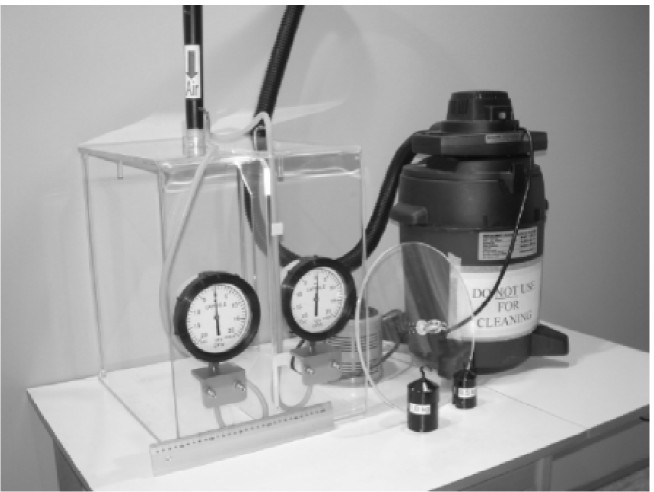
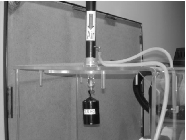
(a) (b)

Figure 1:

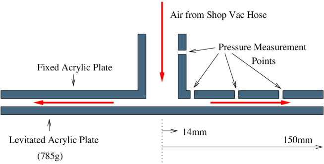
Figure 2:

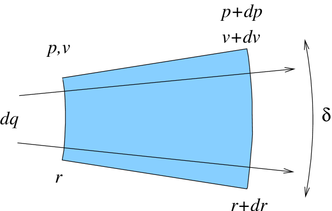
Figure 3:

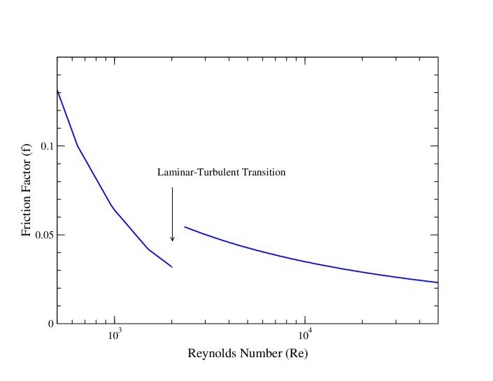
Figure 4:

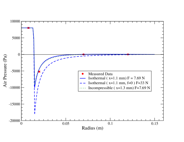
Figure 5:

Figure 6:

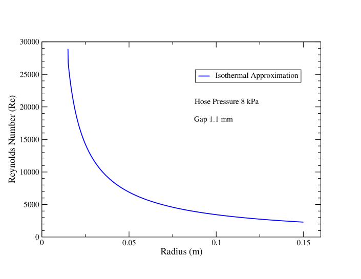
Figure 7:

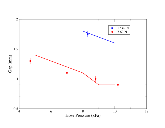
Figure 8:

References

- [1] Jack Murdock Aviation Center, Pearson Field, 1105 E 5th St, Vancouver WA; http://www.ci.vancouver.wa.us/murdock.htm
- [2] Frank M. White, “Fluid Mechanics”, 2nd edition, McGraw-Hill (1986), section 6, p.287ff