Intrabeam scattering analysis of measurements
at KEK’s ATF damping ring

Abstract

We derive a simple relation for estimating the relative emittance growth in $x$ and $y$ due to intrabeam scattering (IBS) in electron storage rings. We show that IBS calculations for the ATF damping ring, when using the formalism of Bjorken-Mtingwa, a modified formalism of Piwinski (where $\eta^{2}/\beta$ has been replaced by ${\cal H}$), or a simple high-energy approximate formula all give results that agree well. Comparing theory, including the effect of potential well bunch lengthening, with a complete set of ATF steady-state beam size vs. current measurements we find reasonably good agreement for energy spread and horizontal emittance. The measured vertical emittance, however, is larger than theory in both offset (zero current emittance) and slope (emittance change with current). The slope error indicates measurement error and/or additional current-dependent physics at the ATF; the offset error, that the assumed Coulomb log is correct to within a factor of 1.75.

I INTRODUCTION

In future e⁺e^- linear colliders, such as the JLC/NLCJLC (1997); The NLC design group (1996), damping rings are needed to generate beams of intense bunches with low emittances. The Accelerator Test Facility (ATF)Hinode et al. (1995) at KEK is a prototype of such damping rings. One of its main goals, and one that has been achieved, was the demonstration of extremely low vertical emittancesKubo et al. (2002); Sakai et al. (2002). At the low ATF emittances, however, it is found that intrabeam scattering (IBS) is a strong effect, and one that needs to be understood.

Intrabeam scattering is an effect that depends on the ring lattice—including the errors—and on all dimensions of the beam, including the energy spread. At the ATF all these dimensions can be measured; unique to the ATF is that the beam energy spread, an especially important parameter in IBS theory, can be measured to an accuracy of a few percent. In April 2000 the single bunch energy spread, bunch length, and horizontal and vertical emittances were all measured as functions of current over a short period of timeUrakawa (2000); Bane et al. (2001). The short period of time was important to ensure that the machine conditions remained unchanged; the bunch length measurement was important since potential well bunch lengthening is significant at the ATFBane et al. (2001). The question that we attempt to answer here is, Are these measurement results in accord with IBS theory?

Intrabeam scattering theory was first developed for accelerators by PiwinskiPiwinski (1974), a result that was extended by MartiniMartini (1984), to give a formulation that we call here the standard Piwinski (P) methodPiwinski (1999); this was followed by the equally detailed Bjorken and Mtingwa (B-M) resultBjorken and Mtingwa (1983). Both approaches solve the local, two-particle Coulomb scattering problem for (six-dimensional) Gaussian, uncoupled beams, but the two results appear to be different; of the two, the B-M result is thought to be the more generalPiwinski . Other simpler, more approximate formulations developed over the years are ones due to ParzenParzen (1987), Le DuffDuff (1989), RaubenheimerRaubenheimer (1991), and WeiWei (1993). Recent reports on IBS theory include one by Kubo and Oide, who adapt an intermediate result from Bjorken-Mtingwa’s paper to find the solution for cases of arbitrary couplingKubo and Oide (2001), a method that is now used in the optics computer program SADOide ; and one by Venturini that solves for IBS in the presence of a strong ring impedanceVenturini (2001).

Intrabeam scattering measurements have been performed primarily on hadronicConte and Martini (1985); Evans and Gareyte (1986); Bhat et al. (1999); Zorzano and Wanzenberg (2000) and heavy ion machinesRao et al. (2000); Fischer et al. (2001), where the effect tends to be more pronounced, though measurement reports on low emittance electron rings can also be foundKim (1998); Steier et al. (2001). Typical of such reports, however, is that although good agreement may be found in some beam dimension(s), the set of measurements and/or agreement is not complete (e.g. in Ref. Conte and Martini (1985) growth rates agree reasonably well in the longitudinal and horizontal directions, but completely disagree in the vertical). Note that one advantage of studying IBS using electron machines is that it can be done by measuring steady-state beam sizes.

In this report we briefly describe intrabeam scattering formulations, apply and compare them for ATF parameters, and finally compare calculations with the full set of data of April 2000. For more details on the hardware and such measurements at the ATF, the reader is referred to Ref. Kubo et al. (2002); Sakai et al. (2002).

II IBS CALCULATIONS

We begin by describing the method of calculating the effect of IBS in a storage ring. Let us first assume that there is no $x$-$y$ coupling.

Let us consider the IBS growth rates in energy $p$, in the horizontal $x$, and in the vertical $y$ to be defined as

$${1\over T_{p}}={1\over\sigma_{p}}{d\sigma_{p}\over dt}\ ,\quad{1\over T_{x}}={1\over\epsilon_{x}^{1/2}}{d\epsilon_{x}^{1/2}\over dt}\ ,\quad{1\over T_{y}}={1\over\epsilon_{y}^{1/2}}{d\epsilon_{y}^{1/2}\over dt}\ .$$ (1)

Here $\sigma_{p}$ is the rms (relative) energy spread, $\epsilon_{x}$ the horizontal emittance, and $\epsilon_{y}$ the vertical emittance. In general, the growth rates are given in both P and B-M theories in the form:

$${1\over T_{i}}=\left<f_{i}\right>$$ (2)

where subscript $i$ stands for $p$, $x$, or $y$. The functions $f_{i}$ are integrals that depend on beam parameters, such as energy and phase space density, and lattice properties, including dispersion; the brackets $\langle\rangle$ mean that the quantity is averaged over the ring. In this report we will primarily use the $f_{i}$ of the B-M formulation.

From the $1/T_{i}$ we obtain the steady-state properties for machines with radiation damping:

$$\epsilon_{x}={\epsilon_{x0}\over 1-\tau_{x}/T_{x}}\ ,\ \epsilon_{y}={\epsilon_{y0}\over 1-\tau_{y}/T_{y}}\ ,\ \sigma^{2}_{p}={\sigma^{2}_{p0}\over 1-\tau_{p}/T_{p}}\ ,$$ (3)

where subscript 0 represents the beam property due to synchrotron radiation alone, i.e. in the absence of IBS, and the $\tau_{i}$ are synchrotron radiation damping times. These are 3 coupled equations since all 3 IBS rise times depend on $\epsilon_{x}$, $\epsilon_{y}$, and $\sigma_{p}$.

The way of solving Eqs. 3 that we employ is to convert them into 3 coupled differential equations, such as is done in e.g. Ref. Kim (1997), and solve for the asymptotic values. For example, the equation for $\epsilon_{y}$ becomes

$${d\epsilon_{y}\over dt}=-{2(\epsilon_{y}-\epsilon_{y0})\over\tau_{y}}+{2\epsilon_{y}\over T_{y}}\quad,$$ (4)

and there are corresponding equations for $\epsilon_{x}$ and $\sigma_{p}^{2}$.

Before solving these equations one needs to know the source of the vertical emittance at zero current. We consider 3 possible sources: (i) vertical dispersion due to vertical orbit errors, (ii) (weak) $x$-$y$ coupling due to such things as rolled quads, etc, and (iii) a combination of the two. If the vertical emittance at zero current is due mainly to vertical dispersion, thenRaubenheimer (1991)

$$\epsilon_{y0}\approx{\cal J}_{\epsilon}\langle{\cal H}_{y}\rangle\sigma_{p0}^{2}\quad,$$ (5)

with ${\cal J}_{\epsilon}$ the energy damping partition number and ${\cal H}=[\eta^{2}+(\beta\eta^{\prime}-{1\over 2}\beta^{\prime}\eta)^{2}]/\beta$ the dispersion invariant, with $\eta$ and $\beta$, respectively, the lattice dispersion and beta functions. If $\epsilon_{y0}$ is mainly due to coupling we drop the $\epsilon_{y}$ differential equation and simply let $\epsilon_{y}=\kappa\epsilon_{x}$, with $\kappa$ the coupling factor. In case (iii) we approximate the solution by replacing the parameter $\epsilon_{y0}$ in Eq. 4 by the quantity [$\kappa\epsilon_{x}(1-\tau_{y}/T_{y})+\epsilon_{y0d}$], where $\epsilon_{y0d}$ is the part of $\epsilon_{y0}$ due to dispersion only. Note that the practice—sometimes found in the literature—of solving IBS equations assuming no vertical errors, which tends to result in near 0 or even negative vertical emittance growth, may describe a state that is unrealistic and unachievable. Note also that in case (i) once the vertical orbit—and therefore $\langle{\cal H}_{y}\rangle$—is set, $\epsilon_{y0}$ is no longer a free parameter.

In addition, note that:

• A fourth equation in our system, the relation between bunch length $\sigma_{s}$ and $\sigma_{p}$, is also implied; generally this is taken to be the nominal (zero current) relation. In the ATF strong potential well bunch lengthening, though no microwave instability, is found at the highest single bunch currentsBane et al. (2001). In our comparisons with ATF measurements we approximate this effect by adding a multiplicative factor $f_{pw}(I)$ [$I$ is current], obtained from measurements, to the equation relating $\sigma_{s}$ to $\sigma_{p}$. (Note that potential well bunch lengthening also changes the longitudinal bunch shape, a less important effect that we will ignore.)

• The B-M results include a so-called Coulomb log factor, $\ln(b_{max}/b_{min})$, with $b_{max}$, $b_{min}$ maximum, minimum impact parameters, quantities which are not well defined. For round beams it seems that $b_{max}$ should be taken as the beam size Farouki and Salpeter (1994). For bi-Gaussian beams it is not clear what the right choice is. Normally $b_{max}$ is taken to be the vertical beams size, though sometimes the horizontal beam size is chosenWei and Parzen (2001). We take $b_{max}=\sigma_{y}$; $b_{min}=r_{0}c^{2}/\langle v_{x}^{2}\rangle$ $=r_{0}\beta_{x}/(\gamma^{2}\epsilon_{x})$, with $r_{0}$ the classical electron radius ($=2.82\times 10^{-15}$ m), $v_{x}$ the transverse velocity in the rest frame, and $\gamma$ the Lorentz energy factor. For the ATF, the Coulomb log, $({\rm log})=16.0$.

• The IBS bunch distributions are not Gaussian, and tail particles can be overemphasized in these solutions. We are interested in core sizes, which we estimate by eliminating interactions with collision rates less than the synchrotron radiation damping rateRaubenheimer (1994). We can approximate this in the Coulomb log term by letting $\pi b_{min}^{2}\langle|v_{x}|\rangle\langle n\rangle$ equal the synchrotron damping rate in the rest frame, with $n$ the particle density in the rest frameKubo and Oide (2001); or $b_{min}=\sqrt{4\pi\sigma_{x}\sigma_{y}\sigma_{z}\gamma/[Nc\tau]}(\beta_{x}/\epsilon_{x})^{1/4}$, with $N$ the bunch population. For the ATF with this cut, $({\rm log})=10.0$.

II.1 High Energy Approximation

For both the P and the B-M methods solving for the IBS growth rates is time consuming, involving, at each iteration step, a numerical integration at every lattice element. A quicker-to-calculate, high energy approximation, one valid in normal storage ring lattices, can be derived from the B-M formalismBane (2002):

$${1\over T_{p}} \approx {r_{0}^{2}cN({\rm log})\over 16\gamma^{3}\epsilon_{x}^{3/4}\epsilon_{y}^{3/4}\sigma_{s}\sigma_{p}^{3}}\left<\sigma_{H}\,g(a/b)\,\left({\beta_{x}\beta_{y}}\right)^{-1/4}\right>$$

$${1\over T_{x,y}} \approx {\sigma_{p}^{2}\langle{\cal H}_{x,y}\rangle\over\epsilon_{x,y}}{1\over T_{p}}\quad,$$ (6)

with

$${1\over\sigma_{H}^{2}}={1\over\sigma_{p}^{2}}+{{\cal H}_{x}\over\epsilon_{x}}+{{\cal H}_{y}\over\epsilon_{y}}\quad,$$ (7)

$$a={\sigma_{H}\over\gamma}\sqrt{\beta_{x}\over\epsilon_{x}}\quad,\quad\quad b={\sigma_{H}\over\gamma}\sqrt{\beta_{y}\over\epsilon_{y}}\quad.$$ (8)

The requirement on high energy is that $a$,$b\ll 1$; if it is satisfied then the beam momentum in the longitudinal plane is much less than in the transverse planes. For flat beams $a/b$ is less than 1. In the ATF, for example, when $\epsilon_{y}/\epsilon_{x}\sim 0.01$, $a\sim 0.01$, $b\sim 0.1$, and $a/b\sim 0.1$. The function $g$, related to the elliptic integral, can be well approximated by

$$g(\alpha)\approx\alpha^{(0.021-0.044\ln\alpha)}\quad\quad[{\rm for}\ 0.01<\alpha<1]\ ;$$ (9)

to obtain $g$ for $\alpha>1$, note that $g(\alpha)=g(1/\alpha)$.

Note that Parzen’s high energy formula is a similar, though more approximate, result to that given hereParzen (1987); and Raubenheimer’s approximation is formulas similar, though less accurate, than the first and identical to the 2nd and 3rd of Eqs. 6Raubenheimer (1991). Note that Eqs. 6 assume that $\epsilon_{y0}$ is due mainly to vertical dispersion; if it is due mainly to $x$-$y$ coupling we let ${\cal H}_{y}=0$, drop the $1/T_{y}$ equation, and simply let $\epsilon_{y}=\kappa\epsilon_{x}$. Finally, note that these equations still need to be iterated, as described before, to find the steady-state solutions.

II.2 Emittance Growth Theorem

Following an argument in Ref. Raubenheimer (1991) we can obtain a relation between the expected vertical and horizontal emittance growth due to IBS in the presence of random vertical dispersion: We begin by noting that the beam momentum in the longitudinal plane is much less than in the transverse planes. Therefore, IBS will first heat the longitudinal plane; this, in turn, increases the transverse emittances through dispersion (through ${\cal H}$, as can be seen in the 2nd and 3rd of Eqs. 6), like synchrotron radiation (SR) does. One difference between IBS and SR is that IBS increases the emittance everywhere, and SR only in bends. We can write

$${\epsilon_{y0}\over\epsilon_{x0}}\approx{{\cal J}_{x}\langle{\cal H}_{y}\rangle_{b}\over{\cal J}_{y}\langle{\cal H}_{x}\rangle_{b}}\quad,\quad{\epsilon_{y}-\epsilon_{y0}\over\epsilon_{x}-\epsilon_{x0}}\approx{{\cal J}_{x}\langle{\cal H}_{y}\rangle\over{\cal J}_{y}\langle{\cal H}_{x}\rangle}\ ,$$ (10)

where ${\cal J}_{x,y}$ are damping partition numbers, and $\langle\rangle_{b}$ means averaging is only done over the bends. For vertical dispersion due to errors we expect $\langle{\cal H}_{y}\rangle_{b}\approx\langle{\cal H}_{y}\rangle$. Therefore,

$$r_{\epsilon}\equiv{(\epsilon_{y}-\epsilon_{y0})/\epsilon_{y0}\over(\epsilon_{x}-\epsilon_{x0})/\epsilon_{x0}}\approx{\langle{\cal H}_{x}\rangle_{b}\over\langle{\cal H}_{x}\rangle}\quad,$$ (11)

which, for the ATF is 1.6. If, however, there is only $x$-$y$ coupling, $r_{\epsilon}=1$; if there is both vertical dispersion and coupling, $r_{\epsilon}$ will be between $\langle{\cal H}_{x}\rangle_{b}/\langle{\cal H}_{x}\rangle$ and 1.

II.3 Numerical Comparison

Let us compare the results of the methods P, B-M, and Eq. 6 when applied to the ATF beam parameters and lattice, with vertical dispersion and no $x$-$y$ coupling. We take as parameters those given in Table I, and, for this comparison, let $f_{pw}=1$. In addition we have ${\cal J}_{\epsilon}=1.4$, $\langle\beta_{x}\rangle=3.9$ m, $\langle\beta_{y}\rangle=4.5$ m, $\langle\eta_{x}\rangle=5.2$ cm and $\langle{\cal H}_{x}\rangle=2.9$ mm. To generate vertical dispersion we randomly offset magnets by 15 $\mu$m, and then calculate the closed orbit using SAD. For our seed we find that the rms dispersion $(\eta_{y})_{rms}=7.4$ mm, $\langle{\cal H}_{y}\rangle=17$ $\mu$m, and $\epsilon_{y0}=6.9$ pm (in agreement with Eq. 5). For consistency between the methods we here take the cut-off parameter $d=3\sigma_{y}$ in P to corresponds to $({\rm log})=\ln{[d\sigma_{H}^{2}/(4r_{0}a^{2})]}=16$ in B-M.

Table 1: Typical ATF parameters in single bunch mode.

Circumference	$C$	138	m
Energy	$E$	1.28	GeV
Current	$I$	3.1	mA
Nominal energy spread	$\sigma_{p0}$	$5.44$	$10^{-4}$
Nominal horizontal emittance	$\epsilon_{x0}$	1.05	nm
Nominal bunch length	$\sigma_{s0}$	5.06	mm
Longitudinal damping time	$\tau_{p}$	20.9	ms
Horizontal damping time	$\tau_{x}$	18.2	ms
Vertical damping time	$\tau_{y}$	29.2	ms

Performing the calculations, but first comparing the standard Piwinski and the B-M methods, we find that the growth rates in $p$ and $x$ agree well; the vertical rate, however, does not. In Fig. 1 we display the local IBS growth rate in $y$ over half the ring (the periodicity is 2), as obtained by the two methods, and see that the P result, on average, is 25% low. Studying the two methods we note that a conspicuous difference between them is their dependence on dispersion: for P the $f_{i}$ depend on it only through $\eta^{2}/\beta$; for B-M, through $\phi=[\eta^{\prime}-{1\over 2}\beta^{\prime}\eta/\beta]$ and through ${\cal H}$. Let us replace $\eta^{2}/\beta$ in P with ${\cal H}$ to create a method that we call the modified Piwinski result. In Ref. Bane (2002) it is shown that, in a normal storage ring lattice, at high energies, the results of this method become equal to those of B-M.

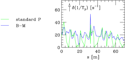
Figure 1: Vertical steady-state (local) growth rate over 1/2 the ATF for an example with vertical dispersion due to random errors. Given are results due to standard Piwinski (green) and Bjorken-Mtingwa (blue).

Comparing with this method we find that, indeed, the three growth rates now agree reasonably well with the B-M result. Fig. 2 displays the 3 local growth rates as obtained by the modified P and B-M methods. The $1/T_{i}$, the average values of these functions, are given in Table II. We note that the P results are all slightly low, by 4.5%. The B-M method gives: $\sigma_{p}/\sigma_{p0}=1.52$, $\epsilon_{x}/\epsilon_{x0}=1.90$, $\epsilon_{y}/\epsilon_{y0}=2.30$. Note that for this error seed the emittance growth ratio of Eq. 11 is $r_{\epsilon}=1.44$, close to the 1.6 expected for the ATF lattice.

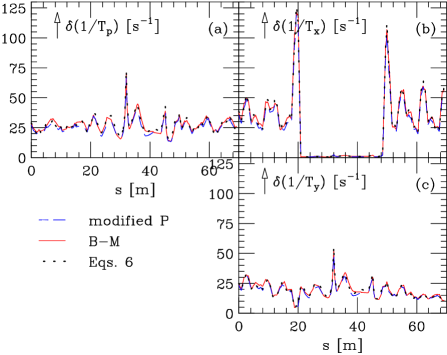
Figure 2: Steady-state (local) growth rates over 1/2 the ATF for an example with vertical dispersion due to random errors. Given are results due to modified Piwinski, Bjorken-Mtingwa, and Eqs. 6.

Table 2: Steady-state IBS growth rates for an example including vertical dispersion due to random errors.

Method	$1/T_{p}$ [s-1]	$1/T_{x}$ [s-1]	$1/T_{y}$ [s-1]
Modified Piwinski	25.9	24.7	18.5
Bjorken-Mtingwa	27.0	26.0	19.4
Eqs. 6	27.4	26.0	19.4

Repeating the calculation using Eqs. 6 we find that the computing time is greatly reduced, and the growth rates agree quite well with the B-M results (see Table II). The dots in Fig. 2 give the local rates corresponding to Eqs. 6, and we see that even these agree quite well.

II.4 Comparison with SAD Results

The optics program SAD basically follows the B-M formalism, but it does it in a form that treats the three beam directions on equal footing. The final results are given in terms of the normal modes of the system and not the beta and dispersion functions of the uncoupled system (as in our approximation). For vertical dispersion dominated problems there is no difference in result. In coupling dominated problems there will be a difference that, in the case of small $x$-$y$ coupling due to errors, we expect to be small.

We consider the ATF lattice with random magnet offsets and rotations. Other machine parameters are the same as before; again $I=3.1$ mA. For this lattice $(\eta_{y})_{rms}=7.4$ mm and $\epsilon_{y0}/\epsilon_{x0}=1\%$. For this problem we solve IBS using SAD (for 2 different seeds), and also our approximate method where we include vertical dispersion (as before) and a global coupling parameter $\kappa=0.34\%$. We take $({\rm log})=9.1$. Comparing steady-state local growth rates, we find good agreement in $p$ and $x$ for all three calculations. In $y$, however, there is a significant variation (see Fig. 3). The growth rates, the average values of these functions, however, agree well (see Table III). Note that the steady-state relative growths in ($\sigma_{p}$,$\epsilon_{x}$,$\epsilon_{y}$) are (1.38,1.56,1.64) for SAD, and (1.38,1.62,1.61) for our approximate calculation.

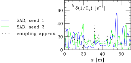
Figure 3: Vertical steady-state (local) growth rate over 1/2 the ATF for an example with vertical dispersion and $x$-$y$ coupling due to random errors. Given are results obtained by SAD (for 2 seeds; the solid curves) and by the coupling approximation used here (the dots).

Table 3: Steady-state IBS growth rates for an example including vertical dispersion and $x$-$y$ coupling due to random errors.

Method	$1/T_{p}$ [s-1]	$1/T_{x}$ [s-1]	$1/T_{y}$ [s-1]
SAD, seed 1	22.5	19.6	13.1
SAD, seed 2	22.3	19.6	13.5
Our approx. calculation	22.9	21.0	12.9

III COMPARISON WITH MEASUREMENT

III.1 Measurements

At the ATF the energy spread and all beam sizes can be measured. Unique at the ATF is that the energy spread, a particularly important parameter in IBS theory, can be obtained to a few percent accuracy. In this measurement the beam is extracted and its size measured on a screen in a highly dispersive region. The bunch length is determined with a streak camera in the ring. The emittances can be measured using 3 methods: wire monitors in the extraction line, a laser wire in the ring, and an interferometer in the ring. Unfortunately, for $\epsilon_{y}$ all 3 methods have their difficulties. For example, the wire measurement is very sensitive to optics errors (such as roll and dispersion) in the extraction line. Or, the laser wire measurement, being time consuming (taking $\sim 1$ hour per measurement), is sensitive to drifts in machine and beam properties.

Because of the effects of IBS the energy spread measurement (which is quick and easy to perform) has become a useful technique for monitoring changes in beam size. Thus, evidence that we are truly seeing IBS at the ATF include: (1) when moving onto the coupling resonance, the normally large energy spread growth with current becomes negligibly small; (2) if we decrease the vertical emittance using dispersion correction, the energy spread increases.

III.2 Comparison with Theory

In Fig. 4, as an example, we present the time development, after injection, of energy spread for 3 different beam currents (the plotting symbols). The measurement was performed by continually injecting beam into the ATF, while varying the extraction timing. If we take the B-M formalism, with $f_{pw}=1$, and with $x$-$y$ coupling 0.006, and solve the differential equations for energy spread and beam sizes, we obtain the curves in the figure (if we include potential well distortion the fitted coupling becomes 0.0045). The short time ($\lesssim 0.05$ s) behavior does not agree with the data, since the beam in reality enters the ring badly mismatched (a region which would be difficult to simulate); in the longer time range, however, after $\gtrsim 3\tau_{p}$, the agreement becomes quite good. The minimum in the curves can be explained as follows: Initially the energy spread and beam sizes reduce due to synchrotron radiation; when the beam volume becomes smaller than a certain amount, the energy spread begins to increase due to IBS. This result indicates reasonably good agreement between measurement and theory.

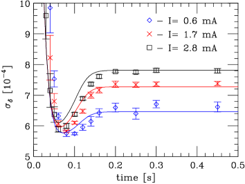
Figure 4: Measured energy spread as function of time after injection, for 3 different currents (the plotting symbols). The curves give B-M simulations assuming an $x$-$y$ coupling of 0.006 and no potential well distortion. This plot is reproduced from Ref. Kubo et al. (2002).

To compare with theory absolutely, however, we need to measure all beam properties with the machine in the same condition. Such a complete series of measurements was performed on stored beam at the ATF over a short period of time in April 2000. The rf voltage was $V_{c}=300$ kV. The energy spread and bunch length vs. current measurements are shown in Fig. 5. The curves in the plots are fits that give the expected zero current result. Emittances were measured on the wire monitors in the extraction line (the symbols in Fig. 6b-c; note that the symbols in Fig. 6a reproduce the fits to the data of Fig. 5). We see large growth also in the emittances. Unfortunately, we have no error bars for the emittance measurements, though we expect the random component of errors in $y$ to be 5-10%, and less in $x$. Note that $\epsilon_{y0}$ appears to be about 1.0-1.2% of $\epsilon_{x0}$.

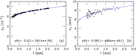
Figure 5: Measurements of steady-state energy spread (a) and bunch length (b), with $V_{c}=300$ kV.

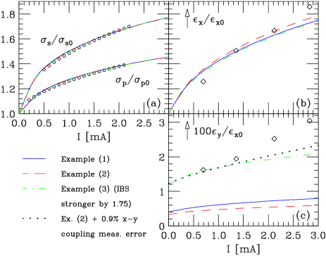
Figure 6: ATF measurement data (symbols) and IBS theory fits (the curves). The symbols in (a) give the smooth curve fits to the measured data of Fig. 5.

Let us compare B-M calculations with the data. Here we take $f_{pw}$ as given by the measurements, and take as Coulomb log our best estimate, $({\rm log})=10$. Note that in the machine the residual dispersion is typically $(\eta_{y})_{rms}\sim 3$ mm. To set our one free parameter, $\epsilon_{y0}$, we adjust it until at high current $\sigma_{p}$ agrees with the measurement. In Fig. 6 we give examples:

1. Vertical dispersion only, with $(\eta_{y})_{rms}=5.6$ mm and $\epsilon_{y0}=4.0$ pm (solid);

2. Coupling dominated with $\kappa=0.33\%$ (dashes);

3. Coupling dominated with $\kappa=1.2\%$, with the Coulomb log artificially increased by a factor 1.75 (dotdash);

4. Same as Ex. 2 but assuming $\epsilon_{y}$ measurement error, i.e. adding 0.9% of the measured (and splined) $\epsilon_{x}$ to the calculated $\epsilon_{y}$ (the dots).

We see that $\sigma_{p}(I)$ agrees well with the measurements for all cases, and $\epsilon_{x}(I)$ agrees reasonably well. For Examples 1 and 2, however, $\epsilon_{y0}$ is significantly lower than the measurements seem to indicate, and the growth with current is also less. To obtain reasonable agreement for $\epsilon_{y0}$ we need to assume that either IBS is $\sim 75\%$ stronger (in growth rates) than theory predicts, or there is significant measurement error, equivalent to $\sim 1\%$ $x$ emittance coupling into the $y$ measurement. Yet even with such assumptions the $\epsilon_{y}(I)$ dependence does not agree.

What does the emittance growth theorem of Sec. II.2 say about these results? It appears that $\epsilon_{x}$ grows by $\sim 85\%$ by $I=3$ mA; $\epsilon_{y}$ begins at about 1.0-1.2% of $\epsilon_{x0}$, and then grows to about 3% of $\epsilon_{x0}$. Therefore, the relative emittance growth ratio is $r_{\epsilon}\sim 2.1$–2.4, much larger than the expected result if we are coupling dominated (1.0); and still significantly larger than the expected result if we are dispersion dominated (1.6), a case that is anyway unlikely since it requires an implausibly large $(\eta_{y})_{rms}\approx 9$ mm. Thus, the emittance growth theorem indicates that $\epsilon_{y}(I)$ as measured is not in agreement with IBS theory.

IV DISCUSSION

Our disagreement in $\epsilon_{y}$ between theory and measurement consists of two parts, an offset part ($\epsilon_{y0}$) and a disagreement in slope ($d\epsilon_{y}/dI$). Together they indicate that we have: error in theory, additional physics at the ATF, and /or error in measurement.

IBS theory is a mature theory, and the relation between longitudinal and transverse growth rates (the 2nd and 3rd of Eqs. 6) is simple and intuitively easy to understand. The main uncertainty in theory may be with the scale factor, particularly in the Coulomb log factor for beams with elliptical cross-section. Yet a scale factor error can affect only the offset part of the disagreement. Note also that even if the argument of (log) were in error by an order of magnitude this part of the disagreement would be changed by only a small amount (25%).

The disagreement in $d\epsilon_{y}/dI$ might be explained by the presence of additional current-dependent physics at the ATF. We have seen that $\sigma_{p}(I)$ and $\epsilon_{x}(I)$ can be made to agree reasonably well between theory and measurement; at the same time, however, the measured $\epsilon_{y}(I)$ grows much faster than predicted. One might, therefore, suspect the presence at the ATF of another current-dependent effect, one that increases the projected vertical emittance—though not the real emittance. An example of such an effect is a $y$-$z$ tilt of the beam induced by closed orbit distortion in the presence of a transverse impedanceChao and Kheifets (1983); Raubenheimer (1991). More study needs to be done in this direction.

As mentioned before, measuring accurately the small vertical emittances at the ATF is difficult, and, therefore, emittance measurement error is likely responsible for much of the disagreement found. We noted that a 1% coupling measurement error in the extraction line wire measurements can account for the offset part of the disagreement; the slope disagreement, however, is not easy to explain assuming measurement error alone (for an attempt in this direction, see e.g. Ref. Ross and Bane (2001)).

Over the time since April 2000 the systematics of the emittance measurements have improved, especially for the laser wire measurement. Newer results seem to suggest that the April 2000 measured vertical emittance may have been too largeKubo et al. (2002); Sakai et al. (2002). For the near future we urge that the effort to obtain reliable emittance measurements at the ATF be continued. In addition, experiments to study the possible existence of other current-dependent effects should also be performed. Ultimately, one goal should be to test the accuracy of theoretical IBS growth rates to the 10–20% level. Note that once we are successful at such benchmarking experiments, we will be able to use the ATF energy spread measurement as a diagnostic for the absolute emittances of the beam.

V CONCLUSION

We began by describing intrabeam scattering calculations for electron storage rings, focusing on machines with small random magnet offset and roll errors. We derived a simple relation for estimating the relative emittance growth in $x$ and $y$ due to IBS in such machines. We have shown that IBS calculations for the ATF damping ring, when using the formalism of Bjorken-Mtingwa, a modified formalism of Piwinski (where $\eta^{2}/\beta$ has been replaced by ${\cal H}$), or a simple high-energy approximate formula all give results that agree well. By comparing with numerical results from SAD we have demonstrated that weak coupling due to random magnet roll can be approximated by solving the uncoupled problem with the addition of a global coupling parameter.

Comparing the B-M calculations, and including the effect of potential well bunch lengthening, with a complete set of ATF steady-state energy spread and beam size vs. current measurements we have found reasonably good agreement in energy spread and horizontal emittance. At the same time, however, we find that the measured vertical emittance is larger than theory in both offset (zero current emittance) and slope (emittance change with current). The slope error indicates measurement error and/or the presence of additional current-dependent physics at the ATF. The offset error suggests that the assumed Coulomb log is correct to within a factor of 1.75 (though we believe that it is, in fact, more accurate, with part of the discrepancy due to measurement error). More study is needed.