A SIMPLIFIED MODEL OF INTRABEAM SCATTERING

Abstract

Beginning with the general Bjorken-Mtingwa solution, we derive a simplified model of intrabeam scattering (IBS), one valid for high energy beams in normal storage rings; our result is similar, though more accurate than a model due to Raubenheimer. In addition, we show that a modified version of Piwinski’s IBS formulation (where $\eta^{2}_{x,y}/\beta_{x,y}$ has been replaced by ${\cal H}_{x,y}$) at high energies asymptotically approaches the same result.

Abstract

Beginning with the general Bjorken-Mtingwa solution, we derive a simplified model of intrabeam scattering (IBS), one valid for high energy beams in normal storage rings; our result is similar, though more accurate than a model due to Raubenheimer. In addition, we show that a modified version of Piwinski’s IBS formulation (where $\eta^{2}_{x,y}/\beta_{x,y}$ has been replaced by ${\cal H}_{x,y}$) at high energies asymptotically approaches the same result.

1 INTRODUCTION

Intrabeam scattering (IBS), an effect that tends to increase the beam emittance, is important in hadronic[1] and heavy ion[2] circular machines, as well as in low emittance electron storage rings[3]. In the former type of machines it results in emittances that continually increase with time; in the latter type, in steady-state emittances that are larger than those given by quantum excitation/synchrotron radiation alone.

The theory of intrabeam scattering for accelerators was first developed by Piwinski[4], a result that was extended by Martini[5], to give a formulation that we call here the standard Piwinski (P) method[6]; this was followed by the equally detailed Bjorken and Mtingwa (B-M) result[7]. Both approaches solve the local, two-particle Coulomb scattering problem for (six-dimensional) Gaussian, uncoupled beams, but the two results appear to be different; of the two, the B-M result is thought to be the more general[8].

For both the P and the B-M methods solving for the IBS growth rates is time consuming, involving, at each time (or iteration) step, a numerical integration at every lattice element. Therefore, simpler, more approximate formulations of IBS have been developed over the years: there are approximate solutions of Parzen[9], Le Duff[10], Raubenheimer[11], and Wei[12]. In the present report we derive—starting with the general B-M formalism—another approximation, one valid for high energy beams and more accurate than Raubenheimer’s approximation. We, in addition, demonstrate that under these same conditions a modified version of Piwinski’s IBS formulation asymptotically becomes equal to this result.

2 HIGH ENERGY APPROXIMATION

2.1 The General B-M Solution[7]

Let us consider bunched beams that are uncoupled, and include vertical dispersion due to e.g. orbit errors. Let the intrabeam scattering growth rates be

$${1\over T_{p}}={1\over\sigma_{p}}{d\sigma_{p}\over dt}\ ,\quad{1\over T_{x}}={1\over\epsilon_{x}^{1/2}}{d\epsilon_{x}^{1/2}\over dt}\ ,\quad{1\over T_{y}}={1\over\epsilon_{y}^{1/2}}{d\epsilon_{y}^{1/2}\over dt}\ ,$$ (1)

with $\sigma_{p}$ the relative energy spread, $\epsilon_{x}$ the horizontal emittance, and $\epsilon_{y}$ the vertical emittance. The growth rates according to Bjorken-Mtingwa (including a $\sqrt{2}$ correction factor[13], and including vertical dispersion) are

$${1\over T_{i}}\ =\ 4\pi A({\rm log})\bigg{<}\int_{0}^{\infty}{d\lambda\,\lambda^{1/2}\over[{\rm det}(L+\lambda I)]^{1/2}}\bigg{\{}$$

$$TrL^{(i)}Tr\left({1\over L+\lambda I}\right)-\ 3TrL^{(i)}\left({1\over L+\lambda I}\right)\bigg{\}}\bigg{>}\quad\ \$$ (2)

where $i$ represents $p$, $x$, or $y$;

$$A={r_{0}^{2}cN\over 64\pi^{2}\bar{\beta}^{3}\gamma^{4}\epsilon_{x}\epsilon_{y}\sigma_{s}\sigma_{p}}\quad,$$ (3)

with $r_{0}$ the classical particle radius, $c$ the speed of light, $N$ the bunch population, $\bar{\beta}$ the velocity over $c$, $\gamma$ the Lorentz energy factor, and $\sigma_{s}$ the bunch length; $({\rm log})$ represents the Coulomb log factor, $\langle\rangle$ means that the enclosed quantities, combinations of beam parameters and lattice properties, are averaged around the entire ring; ${\rm det}$ and $Tr$ signify, respectively, the determinant and the trace of a matrix, and $I$ is the unit matrix. Auxiliary matrices are defined as

$$L=L^{(p)}+L^{(x)}+L^{(y)}\quad,$$ (4)

$$L^{(p)}={\gamma^{2}\over\sigma_{p}^{2}}\left(\begin{array}[]{ccc}0&0&0\\ 0&1&0\\ 0&0&0\end{array}\right)\quad,$$ (5)

$$L^{(x)}={\beta_{x}\over\epsilon_{x}}\left(\begin{array}[]{ccc}1&-\gamma\phi_{x}&0\\ -\gamma\phi_{x}&{\gamma^{2}{\cal H}_{x}/\beta_{x}}&0\\ 0&0&0\end{array}\right)\quad,$$ (6)

$$L^{(y)}={\beta_{y}\over\epsilon_{y}}\left(\begin{array}[]{ccc}0&0&0\\ 0&{\gamma^{2}{\cal H}_{y}/\beta_{y}}&-\gamma\phi_{y}\\ 0&-\gamma\phi_{y}&1\end{array}\right)\quad.$$ (7)

The dispersion invariant is ${\cal H}=[\eta^{2}+(\beta\eta^{\prime}-{1\over 2}\beta^{\prime}\eta)^{2}]/\beta$, and $\phi=\eta^{\prime}-{1\over 2}\beta^{\prime}\eta/\beta$, where $\beta$ and $\eta$ are the beta and dispersion lattice functions.

The Bjorken-Mtingwa Solution at High Energies

Let us first consider $1/T_{p}$ as given by Eq. 2. Note that if we change the integration variable to $\lambda^{\prime}=\lambda\sigma_{H}^{2}/\gamma^{2}$ then

$$(L+\lambda^{\prime}I)={\gamma^{2}\over\sigma_{H}^{2}}\left(\begin{array}[]{ccc}a^{2}+\lambda^{\prime}&-a\zeta_{x}&0\\ -a\zeta_{x}&1+\lambda^{\prime}&-b\zeta_{y}\\ 0&-b\zeta_{y}&b^{2}+\lambda^{\prime}\end{array}\right)\quad,$$ (8)

with

$${1\over\sigma_{H}^{2}}={1\over\sigma_{p}^{2}}+{{\cal H}_{x}\over\epsilon_{x}}+{{\cal H}_{y}\over\epsilon_{y}}\quad,$$ (9)

$$a={\sigma_{H}\over\gamma}\sqrt{\beta_{x}\over\epsilon_{x}}\ ,\quad b={\sigma_{H}\over\gamma}\sqrt{\beta_{y}\over\epsilon_{y}}\ ,\quad\zeta_{x,y}=\phi_{x,y}\sigma_{H}\sqrt{\beta_{x,y}\over\epsilon_{x,y}}$$ (10)

Note that, other than a multiplicative factor, there are only 4 parameters in this matrix: $a$, $b$, $\zeta_{x}$, $\zeta_{x}$. Note that, since $\beta\phi^{2}\leq{\cal H}$, the parameters $\zeta<1$; and that if ${\cal H}\approx\eta^{2}/\beta$ then $\zeta$ is small. We give, in Table 1, average values of $a$, $b$, $\zeta_{x}$, in selected electron rings.

Table 1: Average values of $a$, $b$, $\zeta_{x}$, in selected electron rings. The zero current emittance ratio $\sim 0.5\%$ in all cases.

Machine	$E$[GeV]	$N$[$10^{10}$]	$\langle a\rangle$	$\langle b\rangle$	$\langle\zeta_{x}\rangle$
KEK’s ATF	1.4	.9	.01	.10	.15
NLC	2.0	.75	.01	.20	.40
ALS	1.0	5.	.015	.25	.15

Let us limit consideration to high energies, specifically let us assume $a$,$b\ll 1$ (if the beam is cooler longitudinally than transversely, then this is satisfied). We note that all 3 rings in Table 1, on average, satisfy this condition reasonably well. Assuming this condition, the 2nd term in the braces of Eq. 2 is small compared to the first term, and we drop it. Our second assumption is to drop off-diagonal terms (let $\zeta=0$), and then all matrices will be diagonal.

Simplifying the remaining integral by applying the high energy assumption we finally obtain

$${1\over T_{p}}\approx{r_{0}^{2}cN({\rm log})\over 16\gamma^{3}\epsilon_{x}^{3/4}\epsilon_{y}^{3/4}\sigma_{s}\sigma_{p}^{3}}\left<\sigma_{H}\,g(a/b)\,\left({\beta_{x}\beta_{y}}\right)^{-1/4}\right>\ ,$$ (11)

with

$$g(\alpha)={2\sqrt{\alpha}\over\pi}\int_{0}^{\infty}{du\over\sqrt{1+u^{2}}\sqrt{\alpha^{2}+u^{2}}}\quad.$$ (12)

A plot of $g(\alpha)$ over the interval [$0<\alpha<1$] is given in Fig. 1; to obtain the results for $\alpha>1$, note that $g(\alpha)=g(1/\alpha)$. A fit to $g$,

$$g(\alpha)\approx\alpha^{(0.021-0.044\ln\alpha)}\quad\quad[{\rm for}\ 0.01<\alpha<1]\quad,$$ (13)

is given by the dashes in Fig. 1. The fit has a maximum error of 1.5% over [$0.02\leq\alpha\leq 1$].

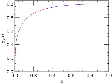
Figure 1: The auxiliary function $g(\alpha)$ (solid curve) and the approximation, $g=\alpha^{(0.021-0.044\ln\alpha)}$ (dashes).

Similarly, beginning with the 2nd and 3rd of Eqs. 2, we obtain

$${1\over T_{x,y}}\approx{\sigma_{p}^{2}\langle{\cal H}_{x,y}\rangle\over\epsilon_{x,y}}{1\over T_{p}}\quad.$$ (14)

Our approximate IBS solution is Eqs. 11,14. Note that Parzen’s high energy formula is a similar, though more approximate, result to that given here[9]; and Raubenheimer’s approximation is Eq. 11, with $g(a/b)\sigma_{H}/\sigma_{p}$ replaced by ${1\over 2}$, and Eqs. 14 exactly as given here[11].

Note that the beam properties in Eqs. 11,14, need to be the self-consistent values. Thus, for example, to find the steady-state growth rates in electron machines, iteration will be required[6]. Note also that these equations assume that the zero-current vertical emittance is due mainly to vertical dispersion caused by orbit errors; if it is due mainly to (weak) $x$-$y$ coupling we let ${\cal H}_{y}=0$, drop the $1/T_{y}$ equation, and let $\epsilon_{y}=\kappa\epsilon_{x}$, with $\kappa$ the coupling factor[3].

What sort of error does our model produce? Consider a position in the ring where $\zeta_{y}=0$. In Fig. 2 we plot the ratio of the local growth rate $T_{p}^{-1}$ as given by our model to that given by Eq. 2 as function of $\zeta_{x}$, for example combinations of $a$ and $b$. We see that for $\zeta_{x}\lesssim\sqrt{b}e^{(1-\sqrt{b})}$ (which is typically true in storage rings) the dependance on $\zeta_{x}$ is weak and can be ignored. In this region we see that the model approaches B-M from above as $a$,$b\rightarrow 0$. Finally, adding small $\zeta_{y}\neq 0$ will reduce slightly the ratio of Fig. 2.

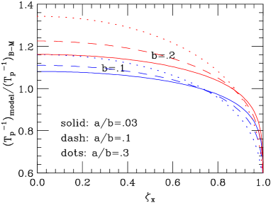
Figure 2: The ratio of local growth rates in $p$ as function of $\zeta_{x}$, for $b=0.1$ (blue) and $b=0.2$ (red) [$\zeta_{y}=0$].

3 COMPARISON TO PIWINSKI

3.1 The Standard Piwinski Solution[6]

The standard Piwinski solution is

$${1\over T_{p}} = A\left<{\sigma_{h}^{2}\over\sigma_{p}^{2}}f(\tilde{a},\tilde{b},q)\right>$$

$${1\over T_{x}} = A\left<f({1\over\tilde{a}},{\tilde{b}\over\tilde{a}},{q\over\tilde{a}})+{\eta_{x}^{2}\sigma_{h}^{2}\over\beta_{x}\epsilon_{x}}f(\tilde{a},\tilde{b},q)\right>$$

$${1\over T_{y}} = A\left<f({1\over\tilde{b}},{\tilde{a}\over\tilde{b}},{q\over\tilde{b}})+{\eta_{y}^{2}\sigma_{h}^{2}\over\beta_{y}\epsilon_{y}}f(\tilde{a},\tilde{b},q)\right>\ ;$$ (15)

$${1\over\sigma_{h}^{2}}={1\over\sigma_{p}^{2}}+{\eta_{x}^{2}\over\beta_{x}\epsilon_{x}}+{\eta_{y}^{2}\over\beta_{y}\epsilon_{y}}\quad,$$ (16)

$$\tilde{a}={\sigma_{h}\over\gamma}\sqrt{\beta_{x}\over\epsilon_{x}},\quad\tilde{b}={\sigma_{h}\over\gamma}\sqrt{\beta_{y}\over\epsilon_{y}},\quad q=\sigma_{h}\beta\sqrt{{2d\over r_{0}}}\quad;$$ (17)

the function $f$ is given by:

$$f(\tilde{a},\tilde{b},q) = 8\pi\int_{0}^{1}du\,{1-3u^{2}\over PQ}\ \times$$ (18)

$$\times \left\{2\ln\left[{q\over 2}\left({1\over P}+{1\over Q}\right)\right]-0.577\ldots\right\}$$

$$P^{2}=\tilde{a}^{2}+(1-\tilde{a}^{2})u^{2},\quad\quad Q^{2}=\tilde{b}^{2}+(1-\tilde{b}^{2})u^{2}\ .$$ (19)

The parameter $d$ functions as a maximum impact parameter, and is normally taken as the vertical beam size.

3.2 Comparison of Modified Piwinski to the B-M Solution at High Energies

We note that Piwinski’s result depends on $\eta^{2}/\beta$, and not on $\cal H$ and $\phi$, as the B-M result does. This may suffice for rings with $\langle{\cal H}\rangle\approx\langle\eta^{2}/\beta\rangle$. For a general comparison, however, let us consider a formulation that we call the modified Piwinski solution. It is the standard version of Piwinski, but with $\eta^{2}/\beta$ replaced by ${\cal H}$ (i.e. $\tilde{a}$, $\tilde{b}$, $\sigma_{h}$, become $a$, $b$, $\sigma_{H}$, respectively).

Let us consider high energy beams, i.e. let $a$,$b\ll 1$: First, notice that in the integral of the auxiliary function $f$ (Eq. 18): the $-0.577$ can be replaced by 0; the $-3u^{2}$ in the numerator can be set to 0; $P$ ($Q$) can be replaced by $\sqrt{a^{2}+u^{2}}$ ($\sqrt{b^{2}+u^{2}}$). The first term in the braces can be approximated by a constant and then be pulled out of the integral; it becomes the effective Coulomb log factor. Note that for the proper choice of the Piwinski parameter $d$, the effective Coulomb log can be made the same as the B-M parameter $({\rm log})$. For flat beams ($a\ll b$), the Coulomb log of Piwinski becomes $({\rm log})=\ln{[d\sigma_{H}^{2}/(4r_{0}a^{2})]}$.

We finally obtain, for the first of Eqs. 15,

$${1\over T_{p}}\approx{r_{0}^{2}cN({\rm log})\over 16\gamma^{3}\epsilon_{x}^{3/4}\epsilon_{y}^{3/4}\sigma_{s}\sigma_{p}^{3}}\left<\sigma_{H}\,h(a,b)\,\left({\beta_{x}\beta_{y}}\right)^{-1/4}\right>\ ,$$ (20)

with

$$h(a,b)={2\sqrt{ab}\over\pi}\int_{0}^{1}{du\over\sqrt{a^{2}+u^{2}}\sqrt{b^{2}+u^{2}}}\quad.$$ (21)

We see that the the approximate equation for $1/T_{p}$ for high energy beams according to modified Piwinski is the same as that for B-M, except that $h(a,b)$ replaces $g(a/b)$. But for $a$,$b$ small, $h(a,b)\approx g(a/b)$, and the Piwinski result approaches the B-M result. For example, for the ATF with $\epsilon_{y}/\epsilon_{x}\sim 0.01$, $a\sim 0.01$, $a/b\sim 0.1$, and $h(a,b)/g(a/b)=0.97$; the agreement is quite good.

Finally, for the relation between the transverse to longitudinal growth rates according to modified Piwinski: note that for non-zero vertical dispersion the second term in the brackets of Eqs. 15 (but with $\eta^{2}_{x,y}/\beta_{x,y}$ replaced by ${\cal H}_{x,y}$), will tend to dominate over the first term, and the results become the same as for the B-M method.

In summary, we have shown that for high energy beams ($a$,$b\ll 1$), in normal rings ($\zeta$ not very close to 1): if the parameter $d$ in P is chosen to give the same equivalent Coulomb log as in B-M, then the modified Piwinski solution agrees with the Bjorken-Mtingwa solution.

4 NUMERICAL COMPARISON[3]

We consider a numerical comparison between results of the general B-M method, the modified Piwinski method, and Eqs. 11,14. The example is the ATF ring with no coupling; to generate vertical errors, magnets were randomly offset by 15 $\mu$m, and the closed orbit was found. For this example $\langle{\cal H}_{y}\rangle=17$ $\mu$m, yielding a zero-current emittance ratio of 0.7%; the beam current is 3.1 mA. The steady-state growth rates according to the 3 methods are given in Table 2. We note that the Piwinski results are 4.5% low, and the results of Eqs. 11,14, agree very well with those of B-M. Additionally, note that, not only the (averaged) growth rates, but even the local growth rates around the ring agree well for the three cases. Finally, note that for coupling dominated NLC, ALS examples ($\kappa=0.5\%$, see Table 1) the error in the steady-state growth rates ($T_{p}^{-1}$,$T_{x}^{-1}$) obtained with the model is (12%,2%), (7%,0%), respectively.

Table 2: Steady-state IBS growth rates (in [s^-1]) for an ATF example with vertical dispersion due to random errors.

Method	$1/T_{p}$	$1/T_{x}$	$1/T_{y}$
Modified Piwinski	25.9	24.7	18.5
Bjorken-Mtingwa	27.0	26.0	19.4
Eqs. 11,14	27.4	26.0	19.4

The author thanks A. Piwinski, K. Kubo and other coauthors of Ref. [3] for help in understanding IBS theory; K. Kubo, A. Wolski, C. Steier, for supplying the lattices of the ATF, NLC, ALS rings, respectively.

References

- [1] C. Bhat, et al, Proc. PAC99, New York (1999) 3155.
- [2] W. Fischer, et al, Proc. PAC2001, Chicago (2001) 2857.
- [3] K. Bane, et al, SLAC-PUB-9227, May 2002.
- [4] A. Piwinski, Tech. Rep. HEAC 74, Stanford, 1974.
- [5] M. Martini, Tech. Rep. PS/84-9(AA), CERN, 1984.
- [6] A. Piwinksi, in Handbook of Accelerator Physics, World Scientific (1999) 125.
- [7] J. Bjorken and S. Mtingwa, Part. Accel., 13 (1983) 115.
- [8] A. Piwinski, private communication.
- [9] G. Parzen, Nucl. Instr. Meth., A256 (1987) 231.
- [10] J. Le Duff, Proc. of CERN Accel. School (1989) 114.
- [11] T. Raubenheimer, SLAC-R-387, PhD thesis, 1991, Sec. 2.3.1.
- [12] J. Wei, Proc. PAC93, Washington, D.C. (1993) 3651.
- [13] K. Kubo and K. Oide, PRST-AB, 4 (2001) 124401.