Noble internal transport barriers and radial subdiffusion of toroidal magnetic lines.

Abstract

Keywords : Tokamak, dynamical system, transport barrier, symplectic mappings, Hamiltonian systems, toroidal magnetic field, subdiffusion, Cantori, noble numbers, plasma confinement, scaling laws

Internal transport barriers (ITB’s) observed in tokamaks are described by a purely magnetic approach. Magnetic line motion in toroidal geometry with broken magnetic surfaces is studied from a previously derived Hamiltonian map in situation of incomplete chaos. This appears to reproduce in a realistic way the main features of a tokamak, for a given safety factor profile and in terms of a single parameter $L$ representing the amplitude of the magnetic perturbation. New results are given concerning the Shafranov shift as function of $L$. The phase space ($\psi,\theta$) of the ”tokamap” describes the poloidal section of the line trajectories, where $\psi$ is the toroidal flux labelling the surfaces. For small values of $L$, closed magnetic surfaces exist (KAM tori) and island chains begin to appear on rational surfaces for higher values of $L$, with chaotic zones around hyperbolic points, as expected. Island remnants persist in the chaotic domain for all relevant values of $L$ at the main rational q-values.

Single trajectories of magnetic line motion indicate the persistence of a central protected plasma core, surrounded by a chaotic shell enclosed in a double-sided transport barrier : the latter is identified as being composed of two Cantori located on two successive ”most-noble” numbers values of the perturbed safety factor, and forming an internal transport barrier (ITB). Magnetic lines which succeed to escape across this barrier begin to wander in a wide chaotic sea extending up to a very robust barrier (as long as $L\precsim 1)$ which is identified mathematically as a robust KAM surface at the plasma edge. In this case the motion is shown to be intermittent, with long stages of pseudo-trapping in the chaotic shell, or of sticking around island remnants, as expected for a continuous time random walk.

For values of $L\succeq 1$, above the escape threshold, most magnetic lines succeed to escape out of the external barrier which has become a permeable Cantorus. Statistical analysis of a large number of trajectories, representing the evolution of a bunch of magnetic lines, indicate that the flux variable $\psi$ asymptotically grows in a diffusive manner as $(L^{2}t)$ with a $L^{2}$ scaling as expected, but that the average radial position $r_{m}(t)$ asymptotically grows as $(L^{2}t)^{1/4}$ while the mean square displacement around this average radius asymptotically grows in a subdiffusive manner as $(L^{2}t)^{1/2}$. This result shows the slower dispersion in the present incomplete chaotic regime, which is different from the usual quasilinear diffusion in completely chaotic situations. For physical times $t_{\varphi}$ of the order of the escape time defined by $x_{m}(t_{\varphi})\sim 1$, the motion appears to be superdiffusive, however, but less dangerous than the generally admitted quasi-linear diffusion. The orders of magnitude of the relevant times in Tore Supra are finally discussed.

PACS numbers: 52.55.Fa, 05.45.+b, 52.25.Gj, 05.40.+j, 52.35.Fp

1 Introduction

The ideal picture of perfect axisymmetric magnetic surfaces in a toroidal magnetic confinement device like a tokamak, appears to be strongly modified either in presence of field inhomogeneities (e.g. divertors) or of tearing instabilities which result in the appearance of magnetic island chains, with a helical symmetry around the magnetic surfaces. The careful experimental analysis performed by N.J. Lopes Cardozo et al. [1], with a very high spatial resolution on electron temperature $T_{e}$ and density $n_{e}$ radial profiles [2], up to a few times the width of an electron banana orbit, has shown that ”small structures appear across the entire profile, with large magnetic islands occurring when the density disruption limit is approached” as a result of plasma filamentation [3]. He concludes that ”the structures are interpreted as evidence that the magnetic topology in the tokamak discharges is not the paradigmatic nest of perfect flux surfaces, but more complex than that”. Similar results have been obtained on the TJ-II stellarator [4] where the very detailed structure of the $T_{e}$ profile measured along a chord has been observed with a $k^{-4}$ spectrum .

In presence of several island chains, it is well-known that overlapping may occur [5], resulting in the appearance of chaotic zones near hyperbolic points, and even chaotic seas with only island remnants. Equations describing magnetic lines in a torus are expressed in terms of the toroidal coordinate $\zeta$ along the line [6]. This variable $\zeta$ is usually interpreted in analogy with a ”time” variable, so that the Hamiltonian equations for magnetic lines are interpreted as ”equations of motion”. In a situation where island overlapping occurs, the classical picture describes a given magnetic line as ”percolating” through the plasma, wandering in the chaotic sea, remaining almost trapped around island remnants (stickiness) and possibly reaching the plasma edge for increasing values of $\zeta$. In either case, this radial motion of the perturbed magnetic lines is responsible for an increased transport of particles and energy, since in the lowest approximation (with vanishing Larmor radii and vanishing magnetic drifts) charged particles just follow magnetic lines in the real time variable which is $t\sim\zeta$ in this simple case. In the following description of magnetic lines, we mainly describe their so-called ”motion”, for simplicity, in spite of the fact that a magnetic line of course remains static and is just followed in $\zeta$ along the toroidal direction.

It is known that a perturbed magnetic field configuration may sometimes be associated with the appearance of  transport barriers (TB) characterized by a jump in the slope of density or temperature profiles, and a strong anomalous transport in the outside zone. TB could also appear in simulations due a strong velocity shear flow (”zonal flows”), even without magnetic turbulence [7]. In Ref. [2] it is recalled that a strongly reduced ion thermal conductivity has been obtained in various tokamaks, which remains at the neoclassical level over part or even the entire plasma. This is due to the presence of an ion TB, associated with a strong velocity shear and a reduction of the density fluctuation level, which is not the case for electron TB observed due to the thin structures measured on $T_{e}$ [2]. Such structures could be associated with alternative layers of good and bad confinement, localized between local barriers. It is important to stress the fact that transport barriers have been shown to be coupled to the safety factor profile ($q$-profile) and to exist also in ohmic plasmas.

Experiments in Tore-Supra, JT-60U, JET, TFTR and other tokamaks (see review in Ref. [8]) clearly exhibit the influence of the safety factor profile ($q$-profile) on the appearance of internal transport barriers (ITB’s) in tokamaks. For this reason we study here TB in a purely magnetic description. Electron ITB has been maintained during $2$ $s.$ in Tore-Supra [9]. Generally ITB’s are obtained in presence of a reversed magnetic shear, i.e. with a $q$ -profile which presents a local maximum near the magnetic axis, and a minimum $q_{\min}$ typically at a normalized radius of $0.3$ - $0.4$, and then a regular increase towards the edge of the plasma. It is generally believed that ITB’s appear around rational $q$-values, and may even follow the time-evolution of a given magnetic surface $q=2$ for instance in JET [10]. Such ITB’s may have a finite width and one finds an ”ITB layer” [11], defined as a thin layer with large $T_{e}$ gradients [2] inside the ”ITB foot”.

On the other hand, even with a monotonic $q$ -profile , a reduced heat diffusivity $\chi$ has been observed in the core region of the plasma, leading to the idea that ITB may appear even without reversed magnetic shear [12]. This is the simple case we will mainly consider here.

The experimental observation that ITB appear ”near” rational surfaces may seem surprising from a theoretical point of view. Rational surfaces are not densely covered by magnetic lines and thus are the most sensitive ones to plasma instabilities. It is a generic property that rational surfaces, on which field lines close back on themselves after a finite number of toroidal turns, are topologically unstable [13]. Irrational surfaces, on the other hand, are covered by a single magnetic line, in an ergodic way, and appear to be more resistant. In the same way, the appearance of large scale chaotic motion is described in dynamical systems theory by successive destructions of KAM tori, and their transformation into permeable dense sets, called Cantori. The most resistant KAM torus in a chaotic system is of course of crucial importance since it is the last inner barrier preventing large scale motion when the stochasticity parameter is increased. In simple cases it corresponds to a rotational transform (winding number) given by the ”most irrational” number, the Golden number. From theoretical grounds, one can thus expect that irrational surfaces are more resistant to chaos [14] and thus more likely to form a transport barrier, if any. In either case, stability or chaos, the breakup of magnetic surfaces ”is a problem of number theory” [15], as will be verified here again.

In the present work we are mainly concerned with the location of ITB’s in a monotonic $q$-profile which appear naturally in a realistic model for toroidal magnetic lines, called ”tokamap” [16]. The unusual point we find here is that the magnetic perturbation, responsible for the appearance of the magnetic island chains, not only creates a non-vanishing Shafranov shift of the magnetic axis as expected, but also build a locally non-monotonic $q$-profile in the equatorial plane, with a spontaneous local maximum $q_{\max}$ on the magnetic axis, and two local minima. The positions of the ITB found here appear to correspond rather exactly, in the perturbed $q$ -profile , to ”most noble” values of $q$ which are the ”next most” irrational numbers beyond the Golden number [17] [18] . These will appear to correspond to the $q-$position of the internal barriers of the tokamap.

It has already been shown that the magnetic surface corresponding to a $q$-value given by the golden KAM torus is not the most robust barrier in the tokamap [16]. In other systems too, the golden mean is not found to be associated with the last KAM curve and the transition to global stochasticity [19], [20]. Most noble values of $q$ are however the location where we may expect, from KAM theory [21] that the most robust tori are finally destroyed and changed into hardly permeable Cantori, which are thus good candidates to be identified with ITB’s. That is what we will check to occur in the tokamap. This result does not fully agree with the generally admitted idea that ITB’s in tokamaks would always be associated with rational $q$-values, but we have to note that the two Cantori forming the barrier found below are nevertheless observed on both side of a low order rational.

Very interesting theoretical models based on transport across chaotic layers and internal barriers have been proposed to explain precise measurements performed on the RTP tokamak. A model of radial transport in a series of chaotic layers has been developed [22] where the standard magnetic equilibrium, with monotonously increasing $q-$profile, is perturbed by small closed current filaments: a number of filaments are localized on low order rational $q-$values, with suitably chosen values for their finite width and current. These current filaments break the topology of nested flux surfaces and are of course responsible for the appearance of magnetic islands and chaotic regions. Test particle transport is computed and is found to be subdiffusive in such perturbed magnetic field, with a mean square displacement growing like the toroidal angle to the power $\frac{1}{2}$ [63].

A model for inhomogeneous heat transport in a stratified plasma has also been developed. Electron heat transport might of course be locally enhanced across each chain of magnetic islands (corresponding to rational $q$-value) and this could cause the appearance of the plateaux observed in the temperature profile [1] at rational $q$-values, explaining some jumps in the slope of the temperature profile. Such stochastic zones around low order rational chains, could also be limited by permeable Cantori. A simple analysis of heat transport in an inhomogeneous stratified medium shows that the measured values may deviate dramatically from simple linear averages [1]: the global transport description should take into account ”insulating” regions but can ignore ”turbulent” regions of high diffusivity. In such models for electron heat transport [23] [24], a number of transport barriers, with suitably chosen width and local heat conductivity, are assumed to be localized on surfaces with low order rational $q-$values. As a result the large electron heat conductivity, assumed to be constant in the conductivity zone, presents a series of depletions (”$q$-comb model”). This model succeeds to reproduce the changes observed in the temperature profile when scanning the deposition radius $\rho_{dep}$ of electron cyclotron heating (ECH) from  central to far off-axis deposition. The main feature of these measurements [25] is the discontinuous response of the $T_{e}$ profile to a continuous variation of the deposition radius $\rho_{dep}$: five plateaux, in which $T_{e}$ is rather insensitive to changes in $\rho_{dep}$, are separated by sudden transitions occurring for small changes of $\rho_{dep}$.

In all these models, the perturbations are assumed to be localized around low-order rational $q-$values, and even if several parameters have to be adjusted, the assumptions of these successful models are fully compatible [24] with the result obtained here, i.e. the magnetic structure of an ITB as being composed of two noble Cantori.

In Section (2) we present this simple Hamiltonian twist map (”tokaMAP” [16]) which has been proved to describe toroidal magnetic lines in a realistic way for tokamaks. Its derivation is summarized. We restrict ourselves mainly to the case of a monotonic $q$ -profile in the unperturbed configuration. We derive some results concerning the localization of the fixed points, and determine the Shafranov shift. The bifurcations determining the number of fixed points are recalled, with an interesting example related to Kadomtsev’s mechanism of sawtooth instability.

Individual magnetic lines are calculated in Section (3) for very large numbers of iterations, and a threshold region of the stochasticity parameter $L$ is found, above which most lines from the central region actually reach the edge of the plasma (global internal chaos). The motion of a single magnetic line is found to be intermittent, with very long periods of trapping in different regions. The motion can indeed be localized between some layers separated by Cantori which correspond rather precisely to noble numbers in the profile of the perturbed $q$-values around the magnetic axis. The spatial localization of these barriers is discussed in Section (4). We also present in Section (5) the calculation of the flux through the Cantori barriers. A Cantorus is a fractal set of points, of fractal dimension zero in the poloidal plane [26] (or of dimension $1$ in the torus: a single magnetic line). Cantori are known to generally represent local permeable barriers in dynamical systems.

In Section (6) we introduce an set of magnetic lines starting from a very small region (or a constant initial radius) and perform averages over this ensemble of lines. Iterations of the tokamap are interpreted in terms of ”time evolution” describing the toroidal motion of a magnetic line. The average radial motion of the lines is described by calculating the ”time”- dependent average radius and average poloidal flux

$$r_{m}(t)\equiv<r(t)>\text{ \ \ \ \ , \ \ \ }\psi_{m}(t)=<\psi(t)>\text{\ \ \ }$$ (1)

reached by the lines at each time, along with the mean square deviation of the flux coordinate $\psi\sim r^{2}$,

$$MSD_{\psi}(t)\equiv<\left[\psi(t)-\psi_{m}(t)\right]^{2}>$$ (2)

and the dispersion of the radial coordinate with respect to this average radius

$$MSD_{rm}(t)\equiv<\left[r(t)-r_{m}(t)\right]^{2}>$$ (3)

Here the brackets $\left\langle...\right\rangle$ indicate an average over the initial conditions.

The time dependence of these three quantities are analyzed and the existence of an asymptotic regime is exhibited: in this regime we observe a diffusion of the flux coordinate (the variance grows linearly in time) , but a subdiffusion of the spatial motion (the variance $MSD_{rm}(t)$ grows like $t^{1/2}$), and a still slower behavior of the average radius, which grows asymptotically like $r_{m}(t)\sim$ $t^{1/4}$. Simple scaling laws are found to describe the dependence of the corresponding ”diffusion” coefficients as function of the stochasticity parameter $L$. A quasilinear scaling in $L^{2}$ is obtained for the flux diffusion $MSD_{\psi}$ , similarly to what is found in the standard map [27], [28], for which additional oscillations deeply modify this simple quadratic growth. As expected, the subdiffusive radial motion $MSD_{rm}(t)$ has a coefficient characterized by a scaling in $L^{1}$, while the slower radial motion $r_{m}(t)$ is characterized by a scaling in $L^{1/2}$.

We finally discuss the order of magnitude of the relaxation time, the time necessary to reach this asymptotic regime and discuss which regime could describe the magnetic line motion before reaching the plasma edge. The conclusions are summarized in Section (7). Partial results have already been presented in a EPS-ICPP conference and published in [29].

2 Hamiltonian map for toroidal magnetic lines

The unperturbed magnetic field realized in tokamaks is ideally represented by a set of nested toroidal magnetic surfaces wound around a circular magnetic axis. The condition $\mathbf{\nabla.B}=0$ allows us to express the magnetic field in the Clebsch form [6] in terms of the dimensionless toroidal flux $\psi$ and poloidal flux $F$.

$$\mathbf{B=\nabla}\psi\mathbf{\times\nabla}\theta\mathbf{-\nabla}F\mathbf{\times\nabla}\zeta$$ (4)

2.1 Equations of motion for magnetic lines

We use traditional toroidal coordinates $(\psi,\theta,\zeta)$ where $\theta$ and $\zeta$ are the poloidal and toroidal angles, respectively, and $\psi$ is the flux coordinate. From (4) the ”equations of motion” for the magnetic lines are easily derived:

$$\frac{d\psi}{d\zeta}=-\frac{\partial F}{\partial\theta}~{}\text{ , ~{}}\frac{d\theta}{d\zeta}=\frac{\partial F}{\partial\psi}$$ (5)

These equations obviously have a Hamiltonian structure: the toroidal angle $\zeta$ plays the role of ”time”, and the poloidal flux $F$ the role of the Hamiltonian.

In the unperturbed case, $F$ is simply a ”surface function” $F=F(\psi)$ which represents an unperturbed Hamiltonian with one degree of freedom and corresponds to an integrable system:

$$\frac{d\psi}{d\zeta}=0~{}\text{ , }~{}\text{~{} }\frac{d\theta}{d\zeta}=\frac{\partial F(\psi)}{\partial\psi}\equiv W(\psi)$$ (6)

where

$$W(\psi)\equiv 1/q(\psi)=\iota(\psi)/2\pi$$ (7)

is the winding number, the inverse of the safety factor $q(\psi)$. Here the action variable $\psi\sim r^{2}$ labels the magnetic surfaces, it is canonically conjugated to the angle variable $\theta$ .

When a magnetic perturbation is applied, due to internal factors (instabilities, fluctuations) or to external causes (imperfection, divertor coils…), the poloidal flux $F$ becomes in general a function of the three coordinates:

$$F(\psi,\theta,\zeta)=F_{0}(\psi)+L\text{ }\delta F(\psi,\theta,\zeta)$$ (8)

where $L$ is the stochasticity parameter (). The field line equations become

$$\frac{d\psi}{d\zeta}=-L\frac{\partial\delta F(\psi,\theta,\zeta)}{\partial\theta}~{}\text{ , }~{}\text{~{} }\frac{d\theta}{d\zeta}=W(\psi)+L\frac{\partial\delta F(\psi,\theta,\zeta)}{\partial\psi}$$ (9)

corresponding to a Hamiltonian dynamical system with $1\frac{1}{2}$ degrees of freedom, generically non integrable. The perturbation is responsible for the appearance of chaos.

2.2
Hamiltonian maps, twist maps and standard map

In order to avoid long symplectic integration in computing the magnetic line motion from (9), discrete iterative maps have been introduced, specially to study the plasma edge. Many examples in the literature have been quoted in [16]. An explicit iterative two-dimensional map consists in discrete transformations of the form

$$\begin{array}[]{ccc}\psi_{\nu+1}=P(\psi_{\nu},\theta_{\nu})&\text{,}&\theta_{\nu+1}=\Theta(\psi_{\nu},\theta_{\nu})\end{array}$$ (10)

where $\nu$ is a non-negative integer which represents physically the number of large turns around the torus, and where the functions $P(\psi_{\nu},\theta_{\nu})$ and $\Theta(\psi_{\nu},\theta_{\nu})$ are explicit in the ”previous” values $\psi_{\nu}$ and $\theta_{\nu}$.

Such transformations must of course conserve the Hamiltonian structure of the equations (9) : the model should be a Hamiltonian map (i.e. area-preserving or symplectic) and therefore the transformation (10) has to be a canonical transformation of the canonical variables $(\psi$, $\theta)$. In order to derive the map, one thus introduces a general generating function $F(\psi_{\nu+1},\theta_{\nu})$ which allows to write down the map as

$$\begin{array}[]{ccc}\psi_{\nu}=\frac{\partial\text{ }F(\psi_{\nu+1},\theta_{\nu})}{\partial\theta_{\nu}}&\text{,}&\theta_{\nu+1}=\frac{\partial\text{ }F(\psi_{\nu+1},\theta_{\nu})}{\partial\psi_{\nu+1}}\end{array}$$ (11)

which is in an implicit form. (Note that we choose here a generating function of the new momentum $\psi$ and the old angle $\theta$, but the inverse choice is also possible and would lead to another family of maps).

Other choices are possible for the same twist map, for instance with another kind of generating function $F_{a}(\theta_{\nu},\theta_{\nu+1})$ called the action generating function used in Section (5), from which the map can be written as

$$\begin{array}[]{ccc}\psi_{\nu}=-\frac{\partial\text{ }F_{a}(\theta_{\nu},\theta_{\nu+1})}{\partial\theta_{\nu}}&\text{,}&\psi_{\nu+1}=\frac{\partial\text{ }F_{a}(\theta_{\nu},\theta_{\nu+1})}{\partial\theta_{\nu+1}}\end{array}$$ (12)

The relation between $F$ and $F_{a}$ is thus (from (11) and (12)):

$$F_{a}(\theta_{\nu},\theta_{\nu+1})=\psi_{\nu+1}(\theta_{\nu},\theta_{\nu+1}).\theta_{\nu+1}-F\left[\psi_{\nu+1}(\theta_{\nu},\theta_{\nu+1}),\theta_{\nu}\right]$$ (13)

(see Ref. [30]).

2.2.1 General form of a twist map

In order to proceed, the following general form of the generating function has been chosen:

$$F(\psi_{\nu+1},\theta_{\nu})=\psi_{\nu+1}.\theta_{\nu}+F_{0}(\psi_{\nu+1})+L\text{ }\delta F(\psi_{\nu+1},\theta_{\nu})$$ (14)

where $L$ is the perturbation parameter and $F_{0}(\psi_{\nu+1})$ the unperturbed term taking into account the winding number (see(7))

$$W(\psi)=\frac{\partial F_{0}(\psi)}{\partial\psi}\equiv\frac{1}{q(\psi)}$$ (15)

As a consequence of (11) the map takes the following form

$$\psi_{\nu+1}=\psi_{\nu}+L\text{ }h(\psi_{\nu+1},\theta_{\nu})$$

$$\theta_{\nu+1}=\theta_{\nu}+W(\psi_{\nu+1})+L\text{ \ }j(\psi_{\nu+1},\theta_{\nu})$$ (16)

which is an Hamiltonian form because the two functions $h$ and $j$ defined by

$$\begin{array}[]{ccc}h(\psi_{\nu+1},\theta_{\nu})=-\frac{\partial\text{ }\delta F(\psi_{\nu+1},\theta_{\nu})}{\partial\theta_{\nu}}&\text{,}&j(\psi_{\nu+1},\theta_{\nu})=\frac{\partial\text{ }\delta F(\psi_{\nu+1},\theta_{\nu})}{\partial\psi_{\nu+1}}\end{array}$$ (17)

automatically insure that

$$\frac{\partial\text{ }h(\psi_{\nu+1},\theta_{\nu})}{\partial\text{ }\psi_{\nu+1}}+\frac{\partial\text{ }j(\psi_{\nu+1},\theta_{\nu})}{\partial\text{ }\theta_{\nu}}=0$$ (18)

Equations (16) has the form of a general Hamiltonian map, from which simple cases can be recovered.

When variables are clearly separated in (16) i.e. for $h=h(\theta_{\nu})$ and $j=j(\psi_{\nu+1})$ one finds a general twist map in the case where the profile $q(\psi)$ is monotonous (see section 5.1 below).

2.2.2 The standard map

The Chirikov-Taylor standard map[27] [28] belongs to that family and corresponds to

$$\begin{array}[]{ccccc}h(\theta)=-\sin 2\pi\theta&\text{,}&j(\psi)=0&\text{,}&W(\psi)=\psi\end{array}$$ (19)

and has the following form

$$\begin{array}[]{cccc}\psi_{\nu+1}=\psi_{\nu}-L\sin 2\pi\theta_{\nu}&&\text{,}&\text{ }\theta_{\nu+1}=\theta_{\nu}+\psi_{\nu+1}\end{array}$$ (20)

corresponding to

$$\begin{array}[]{ccc}F_{0}(\psi)=\frac{1}{2}\psi^{2}&\text{,}&\delta F(\psi,\theta)=-\frac{1}{2\pi}\cos(2\pi\theta)\end{array}$$ (21)

The generating functions for the standard map are thus

$$F(\psi_{\nu+1},\theta_{\nu})=\psi_{\nu+1}.\theta_{\nu}+\frac{1}{2}\psi_{\nu+1}^{2}-\frac{L}{2\pi}\cos(2\pi\theta_{\nu})$$ (22)

and

$$F_{a}(\theta_{\nu},\theta_{\nu+1})=\frac{1}{2}\left[\theta_{\nu}-\theta_{\nu+1}\right]^{2}+\frac{L}{2\pi}\cos(2\pi\theta_{\nu})\text{ }$$ (23)

2.2.3 The Wobig map

The Wobig map [31] on the other hand corresponds to :

$$\begin{array}[]{ccccc}h(\psi,\theta)=-\psi\sin 2\pi\theta&\text{,}&j(\psi)=-\frac{1}{(2\pi)}\cos 2\pi\theta&\text{,}&W(\psi)=\psi\end{array}$$ (24)

and has the form

$$\begin{array}[]{ccc}\psi_{\nu+1}=\psi_{\nu}-L\psi_{\nu+1}\sin 2\pi\theta_{\nu}&\text{,}&\theta_{\nu+1}=\theta_{\nu}+\psi_{\nu+1}-\frac{L}{(2\pi)}\cos 2\pi\theta_{\nu}\end{array}$$ (25)

corresponding to

$$\begin{array}[]{ccc}F_{0}(\psi)=\frac{1}{2}\psi^{2}&\text{,}&\delta F(\psi,\theta)=-\frac{1}{2\pi}\psi\cos(2\pi\theta)\end{array}$$ (26)

The generating functions for the Wobig map are thus

$$F(\psi_{\nu+1},\theta_{\nu})=\psi_{\nu+1}.\theta_{\nu}+\frac{1}{2}\psi_{\nu+1}^{2}-\frac{L}{2\pi}\psi_{\nu+1}\cos(2\pi\theta_{\nu})$$ (27)

and

$$F_{a}(\theta_{\nu},\theta_{\nu+1})=\frac{1}{2}\left[\theta_{\nu+1}-\theta_{\nu}+\frac{L}{2\pi}\cos(2\pi\theta_{\nu})\right]^{2}\text{ }$$ (28)

These last two maps are actually not suitable to represent magnetic lines in a tokamak first because they do not insure that a nonnegative value of $\psi\sim r^{2}$ remains nonnegative after iteration (as it should to represent a real value of the radial position) and, second, because they do not involve any realistic profile of the winding number $W(\psi)$ (they correspond to a $q$ -profile everywhere decreasing: $q\sim 1/r^{2}).$ In order to satisfy these two necessary properties, another model is described in the next section.

2.3 The tokamap

A specific model, the ”tokamap” has been derived in [16] from general properties of Hamiltonian twist maps. The advantage consists in succeeding to describe the whole body of a tokamak plasma, including chains of magnetic islands in a realistic way. This map describes the basic motion of the magnetic lines in the two dimensional poloidal plane $(\psi,\theta)$ by the winding number $W(\psi)$ which is here modified by an additional contribution from the magnetic perturbation.

The general expression of the tokamap results from the following choice in the generating function (14) :

$$\delta F(\psi_{\nu+1},\theta_{\nu})=-\frac{1}{2\pi}\frac{\psi_{\nu+1}}{1+\psi_{\nu+1}}\cos 2\pi\theta_{\nu}\text{ \ (tokamap)}$$ (29)

which involves an additional $\psi$ dependence as compared to Eq.(26). We thus consider the following generating function for the Tokamap (see (14) and (29)):

$$F(\psi_{\nu+1},\theta_{\nu})=\psi_{\nu+1}.\theta_{\nu}+F_{0}(\psi_{\nu+1})-L\frac{\psi_{\nu+1}}{1+\psi_{\nu+1}}\cos 2\pi\theta_{\nu}\text{ \ (tokamap)}$$ (30)

This immediately leads to the following implicit form of the tokamap (use (11)):

$$\psi_{\nu+1}=\psi_{\nu}-L\frac{\psi_{\nu+1}}{1+\psi_{\nu+1}}\sin(2\pi\theta_{\nu})$$ (31)

$$\theta_{\nu+1}=\theta_{\nu}+W(\psi_{\nu+1})-\frac{L}{2\pi}\frac{1}{(1+\psi_{\nu+1})^{2}}\cos(2\pi\theta_{\nu})$$ (32)

where $\theta$ denotes the poloidal angle divided by $2\pi$ . In this nonlinear map a unique root is chosen for Eq. (31):

$$\psi_{\nu+1}=\frac{1}{2}\left(P(\psi_{\nu},\theta_{\nu})+\sqrt{\left[P(\psi_{\nu},\theta_{\nu})\right]^{2}+4\psi_{\nu}}\right)$$ (33)

where

$$P(\psi,\theta)=\psi-1-L\sin(2\pi\theta)$$ (34)

This explicit map (31-34) has been shown to be compatible with minimal toroidal geometry requirements. The polar axis $(\psi=0)$ represents the magnetic axis in the unperturbed configuration. This map depends on one parameter, the stochasticity parameter $L$ (), and on one arbitrary function $W(\psi)$ which is chosen according to the $q$ -profile we want to represent. For increasing values of $L$, chaotic regions appear mostly near the edge of the plasma.

It is a simple matter to check that the symmetries of the tokamap imply that, for negative values of $L$, the phase portrait is the same as for positive values, but with the simple poloidal translation : $\theta\Rightarrow\theta+1/2$ which means that the original phase portrait for $\theta=0$ to $1$ is recovered identically but for $\theta=-1/2$ to $+1/2$ .

It has been shown that, contrary to what occurs in the Chirikov-Taylor standard map [27] or even in the Wobig map [31], a nonnegative value of $\psi$ always yields a nonnegative iterated value, insuring that the radius remains a real number (see Eq.(123)). In the domain $L<1$, however, the Wobig map also conserves nonnegativity of $\psi$ .

The tokamap has recently been deduced in a very different way [32], as a particular case of a particle map describing guiding centre toroidal trajectories in a perturbed magnetic field given in general by (4), and to lowest order by the standard magnetic field model [33], [34]:

$$\mathbf{B}=\frac{B_{0}}{1+\varepsilon_{T}\text{ }x\cos\theta}\left[\mathbf{e}_{\zeta}+\varepsilon_{T}\frac{x}{q(x)}\mathbf{e}_{\theta}\right]$$ (35)

where $\varepsilon_{T}=a/R_{0}$ is the inverse aspect ratio of the torus, $R_{0}$ the large radius of the torus, $B_{0}$ the magnetic field strength on the axis and $x=\rho/a$ the normalized radial coordinate of the plasma of small radius $a$ . This magnetic field (35) is checked to be divergenceless. By comparing the poloidal flux expressions in the general Clebsch formula (4) and in the above standard model (35), it is easy to deduce that the toroidal flux $\psi$ in this case is given by

$$\psi=\frac{x^{2}}{2}$$ (36)

in the dimensionless units used in the tokamap.

In [32] canonical coordinates for guiding centre have been derived, allowing for the symplectic integration of the equations of motion and the derivation of a Hamiltonian map for guiding centre in a perturbed toroidal geometry. As a particular case, the tokamap is deduced from this particle map when one applies a simple $m=0$ nonresonant magnetic perturbation. In order to describe magnetic line motion only, the magnetic moment is considered to be zero, and one keeps terms to the lowest order in the inverse aspect ratio $\varepsilon_{T}$. Moreover, in order to go from the time dependence of the particle trajectory to the toroidal $\zeta$-dependence of the position $(\psi,\theta)$ of the magnetic line, all equations are simply divided by the equation for $\partial\zeta/\partial t$ . As a result, Eqs.(31-34) are exactly recovered. This derivation also allows to write down explicitly the form of the magnetic perturbation involved in the tokamap : The generating function (14) takes into account a magnetic divergence-free perturbation $\delta\mathbf{B}$ with the following components:

$$\frac{\delta B_{\theta}}{B_{0}}=L.\frac{x.\epsilon_{T}}{h(x,\theta)}.\frac{\partial\text{ }\delta F(\psi,\theta)}{\partial\psi}$$ (37)

and

$$\frac{\delta B_{\rho}}{B_{0}}=-L.\frac{\epsilon_{T}}{x.h(x,\theta)}.\frac{\partial\text{ }\delta F(\psi,\theta)}{\partial\theta}$$ (38)

where $h(x,\theta)=\left(1+\epsilon_{T}.x.\cos\theta\right)$ represents the toroidal effect.

A different but related method of derivation of symplectic maps has been used by Abdullaev [35].

2.3.1 Safety factor profile

In order to take magnetic shear into account, a specific $q$ -profile has to be introduced to describe the unperturbed equilibrium. We consider here the same profile as in Ref. [16] :

$$q(\psi)=\frac{4}{w.(2-\psi).(2-2\psi+\psi^{2})}$$ (39)

which corresponds to a classical cylindrical equilibrium [36] in which the value on the axis ($\psi=0$) is given by the parameter $w$ :

$$q(\psi=0)=\frac{1}{w}$$ (40)

and on the edge ($\psi=1$) by :

$$q(\psi=1)=4q(0)$$ (41)

which is four times the central value. The derivation of this $q$ -profile (39) is presented in Appendix A.

2.3.2 One example with reversed magnetic shear : the ”Rev-tokamap”

If a non monotonic $q$ -profile is used instead, a reversed magnetic shear is introduced in the unperturbed magnetic field, and it has been shown that the above mapping becomes a nontwist map : this ”Rev-tokamap” [37] has very different properties namely because the Kolmogorov-Arnold-Moser (KAM) theorem does not apply anymore. It has been found [37] that a critical surface appears in the plasma near the minimum of the $q$ -profile , separating an external, globally stochastic region from a central, robust nonstochastic core region. Such a phenomena of ”semiglobal chaos” has been shown to be analogous to the appearance of ITB in reversed shear experiments. Later, similar theoretical results have been obtained in the Lausanne group [38] in a reversed shear TEXTOR equilibrium; by studying a symplectic perturbed map for the magnetic topology, they confirmed that the transport barrier is indeed localized near the minimum of the $q$ -profile .

Coming back on the reversed shear model of Ref. [37] we will show below in Section (4.5.2) that the ITB found in that work is also localized with a good precision on a $q$-value which will appear to be a noble number.

2.3.3 Fixed points and bifurcations

The general structure of the phase portrait of the tokamap has been described in detail in [16]. Fixed points of the map should not be confused with secondary magnetic axes inside the islands: the latter are not fixed but wander upon iteration from one island to another island of the chain and appear as periodic points.

Fixed points, defined by $\psi_{\nu+1}=\psi_{\nu}$ and $\theta_{\nu+1}=\theta_{\nu}+n$ where $n$ is an integer, can easily be calculated by using first Eq. (31) which yields either $\psi=0$ (the polar axis) or $\sin(2\pi\theta_{\nu})=0$. This proves that all fixed points are either

- on the polar axis ($\psi=0$), for instance  $\theta=0.25$ and $0.75$ which are two hyperbolic points on the polar axis, and exist as long as $L<1$,

- or in the equatorial plane ($\theta=0$ or $0.5$). By using next Eq. (32), one finds that the values of $\psi$ at the fixed points with $\theta=0$ are solutions of

$$F_{1}(\psi,K,w,n)\equiv W(\psi)-\frac{L}{2\pi}\frac{1}{(1+\psi)^{2}}-n=0$$ (42)

while values of $\psi$ at the fixed points with $\theta=0.5$ are solutions of

$$F_{2}(\psi,K,w,n)\equiv W(\psi)+\frac{L}{2\pi}\frac{1}{(1+\psi)^{2}}-n=0$$ (43)

It has been shown [16] that the origin, the polar axis $(\psi=0)$ is a fixed point as long as $L<1$. Fixed points have been discussed in great detail in [16], including consideration of the ”ghost space” $\psi<0$ which appears necessary in order to check that the Poincaré-Birkhoff theorem and the conservation of stability index (the difference between the number of elliptic and hyperbolic points which remains constant as $w$ varies) are indeed satisfied. Let us simply recall here that bifurcations occur according to the value of $w$ representing the central winding number (see 40) as compared to the following $L$-dependent parameters

$$w_{m}(L)\equiv 1-L$$ (44)

and

$$w_{M}(L)=2-w_{m}=1+L>w_{m}(L)$$ (45)

As long as $w<w_{m}=1-L$, the only invariant point is the polar axis $\psi=0$, which obviously has to be interpreted in this case as the magnetic axis of the tokamak (see Fig. 15 in [16]).

For higher values of $w$, when $w_{m}<w<w_{M}\equiv 2-w_{m}$ , i.e. $1-L<w<1+L$, a first bifurcation has occurred, with the appearance of an elliptic point off the polar axis. This latter elliptic point has to be interpreted as the magnetic axis, displaced by the Shafranov shift [39], [40]. In the case $w=1$ (to which we will restrict ourselves in the next Sections), the position $\psi_{MA}$ of this magnetic axis is obtained by using Eq. (43) as function of $L$ as:

$$F_{2}(\psi_{MA},L,w=1,n=1)=0$$ (46)

The curve giving $\psi=\psi_{MA}(K=2\pi L)$ is plotted in Fig.(1).

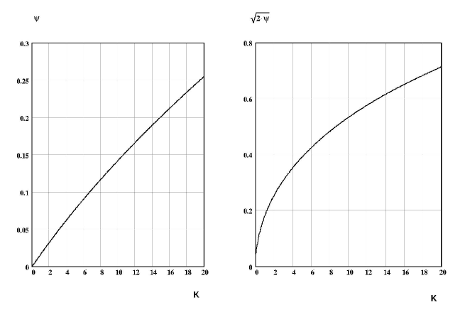
Figure 1: Analytic solution for the Shafranov shift: position $\psi$ of the magnetic axis as function of $K=2\pi L$ in the case $w=1$. For $L=4.875/2\pi$ this formula yields $\psi(L=4.875/2\pi)=0.07492$ . Here $r=\sqrt{\psi}$ represents the radial coordinate, with $r=\sqrt{2}$ on the edge.

In the absence of any perturbation ($L=0$), the magnetic surfaces are centered around the polar axis.

A first typical phase portrait is given in Fig. 5 of Ref. [16] for the simple case where $q(0)=1$, and $L=4.5/2\pi\sim 0.716$ , hence $w=1$ and $w_{m}<w$. One can see the formation of a chaotic belt which surrounds several large islands chains. This belt is clearly confined between two surfaces which were interpreted as KAM surfaces in this case. Several other examples are given below (see Figs.2-5). We will discuss why, for slightly higher values of $L$, such boundary surfaces can be identified as fractal barriers or Cantori, which can be crossed by a magnetic line after a very long time.

2.3.4 Second bifurcation for $q(0)<1$

A second bifurcation occurs for still higher values of $w$ when $w_{m}<w_{M}<w$, i.e. when $1+L<w$  which implies $q(0)<1$ : the magnetic axis remains displaced from the origin and corresponds to the center of a $m=1$ island in the equatorial plane at $\theta=0.5$, resulting in the appearance of an hyperbolic point (”$X$ point”) for $\theta=0$ with a separatrix enclosing the origin. The latter appears to be the ”main” magnetic axis, ”expelled” by the presence of the $m=1$ island. This can be seen in Fig.(2) which presents the tokamap phase portrait for $L=1/4\pi$, $w=1.05$ (thus $q(0)<1$ and $w_{m}<w$) over $N=8193$ iterations.

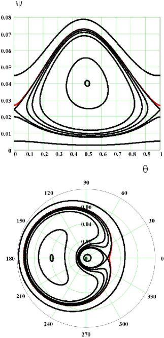
Figure 2: Tokamap phase portrait for $L=0.5/2\pi$ with $q(0)<1$ $(w=1.05$ and $N=8190$). The polar axis $(0,0)$ is the main magnetic axis of the plasma core. The position of the elliptic point in the $m=1$ island is $\psi=0.040246$, $\theta=0.5$ and the hyperbolic point is located in $\psi=0.024481$, $\theta=0$.

This example shows the final situation after a big island $(m=1)$ has grown and expelled a small region around the original magnetic axis near the polar axis; this occurs when the unperturbed $q$-value on the axis is smaller than unity, $q(0)=1/w<1$, allowing for the existence of a surface $q=1$ inside the plasma. It has been stressed that this process occurs as a result of a reconnection of magnetic lines, and is typical of Kadomtsev’s theory of sawtooth instabilities. The position of the $m=1$ magnetic axis (”$O$ point”), as well as the position of the hyperbolic $X$ point can be calculated analytically from Eqs. (42, 43), in agreement with Fig. 17 of Ref. [16]. (We note that two misprints appeared in the text of that paper for the exact numerical values which should be written $\psi 1=$ $0.040$ of the $O$ point, and $\psi 2=0.024$ of the $X$ point, as indicated by the Fig. 17, instead of $0.179$ and $0.167$ written in the main text).

These points can be calculated as follows. For $w_{M}<w$ the position $\psi_{H}$ of the hyperbolic $X$ point is given by the solution of $F_{1}(\psi_{H},L,w,1)=0$ (with $\theta=0$) as defined in Eq. (42). For a given $w$, this solution exists only for the smaller values of $L$. For instance for $w=1.05$ it exists only for $K=2\pi L\leq 1.97392$ , which means that for $q(0)<1$ this $X$ point only appears for small values of the perturbation parameter.

The position $\psi_{E}$ of the $m=1$ magnetic axis (elliptic or $O$ point) is given by the solution of $F_{2}(\psi_{E},L,w,1)=0$ (with $\theta=0.5$). We remark that this last solution $\psi_{E}(L)$ does not vanish for $L\Rightarrow 0$, which would seem to indicate the existence of a fixed point $\left[\psi_{E}(L=0),\theta=0.5\right]$ out of the polar axis $\psi=0$, even in the unperturbed case where all magnetic surfaces are circles centered around the origin… In this case we have $w_{M}(L=0)=1<w$ which means $q(0)<1$ and this fixed point $\left[\psi_{E}(L=0),\theta=0.5\right]$ is simply a standard point of the circular surface $q=1$ : this is just a special feature of this unperturbed surface on which every point appears as stationary since it exactly comes back after one toroidal rotation (one iteration). This specific point with $\theta=0.5$ in the unperturbed case is however important since it acts as a seed for the $m=1$ island which appears when $L$ becomes different from zero. We note that this position $\psi_{E}(L)$ is such that $q(\psi_{E}(L=0))=1$.

In order to simplify the discussion about dispersive motion of the magnetic lines in the tokamap, we will restrict ourselves in the following Sections to the case

$$w=1$$ (47)

which means $q(0)=1$ . The unperturbed $q$ -profile is a continuous and monotonous function, with a value growing from $1$ in the center to $4$ on the edge of the plasma, a rather standard profile in most ohmic discharges. In this case for any $L>0$, we have from Eq. (44) $w_{m}(L)=1-L\leq$ $w$, i.e. we are beyond the first bifurcation and the position of the magnetic axis is given by Fig. (1).

3 Individual trajectories: tokamap phase space portrait

In this section we first present the phase portrait of the tokamap in the case $w=1$, $q(0)=1$ for increasing values of the stochasticity parameter and then study very long trajectories.

3.1 Increasing stochasticity

For increasing values of the stochasticity parameter the tokamap exhibits all the main features of chaotic systems, in a way which is very realistic for tokamaks.

3.1.1 Weak stochasticity regime : confinement by KAM tori

For small values of the stochasticity parameter $L=K/2\pi<<1$, most of the KAM surfaces are preserved and the phase portrait of the tokamap appears to be described by embedded tori, around a magnetic axis displaced from the origin $(\psi=0,\theta=0)$ by the Shafranov shift (46), as seen in Fig.(3).

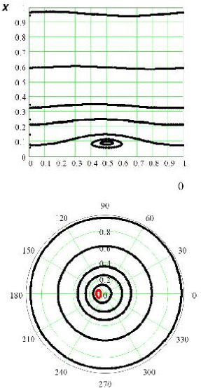
Figure 3: Regular KAM magnetic surfaces with a Shafranov shift for a small value of the stochasticity parameter $L=0.08$, with $w=1$. The angle $\theta$ is represented modulo $2\pi$.

In this case all magnetic lines remain confined, no magnetic island is seen. From the position of the shifted magnetic axis, we note that, for positive values of $L$, the weak field side of the torus is in the direction $\theta=0.5$ .

3.1.2 Appearance of island chains on rational $q$-values

For an increased value of $L$, regular chains of magnetic islands appear; their number $m$ and the order in which these islands are visited by a magnetic line allow us to deduce their $q$-value in a simple way. For instance a chain of $m$ islands visited one by one at each iteration, in the direction of increasing values of $\theta$, has a rotational transform or winding number $\iota(\psi)/2\pi$ equal to $1/m$, and a $q$-value $q=m$. These are the main island chains, as seen in Fig.(4).

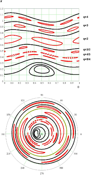
Figure 4: Regular KAM tori for $L=0.4$, $w=1$, and main rational island chains corresponding to $q=5/4$, $4/3$, $3/2$, $2$, $3$ and $4$

A direct measurement of the exact value of $q$ can be performed, specially for almost undestroyed magnetic surfaces, by computing the average winding number along a trajectory, see (7).  For small circles around the magnetic axis (which do not encircle the polar axis), a change of coordinate is necessary to evaluate correctly the rotation around the magnetic axis. On the other hand, for all surfaces encircling the polar axis, the knowledge of the iterated values $\theta_{\tau}$ allows us to calculate the following surface quantity (average on a given magnetic surface)

$$\left\langle\iota/2\pi\right\rangle=\lim_{N\rightarrow\infty}\frac{1}{N}\sum_{\tau=1}^{\tau=N}\left(\theta_{\tau}-\theta_{\tau-1}\right)$$ (48)

which is the average increase of the poloidal angle over a large number $N$ of iterations. The $q-$value of the corresponding trajectory is immediately obtained from (7).

3.1.3 Overlapping chains, secondary islands and chaotic regions

For an increased stochasticity parameter $L=4.875/2\pi\sim 0.776$ , the same initial conditions as in Fig.(4) actually describe a wide chaotic zone surrounding a central part with regular KAM tori : see Fig.(5).

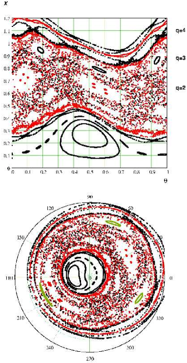
Figure 5: With the same initial conditions as in Fig. 4 $(w=1)$ with a higher value of the stochasticity parameter $L=4.875/2\pi\sim 0.776$, regular KAM tori are observed in the central part, while the main rational island chains corresponding to $q=$ $3/2$, $2$, $3$ and $4$ are stochastized.

The main rational chains $q=3/2$, $2$, $3$ and $4$ are partly stochastized.

We show on Fig.(6) a small part of the phase portrait obtained by following $6$ trajectories along $16$ $380$ iterations: the main chain of primary islands is observed, with intermediate higher rational chains, surrounded by stochastic regions in the vicinity of the hyperbolic points (as usual in nonlinear dynamical systems).

Figure 6: Partial vue of the phase portrait with six trajectories for $L=4.875/2\pi\sim 0.776$, which shows the structures of rational chains of island remnants and the stochastic web expanding from the hyperbolic points.

3.1.4 Island remnants in the chaotic sea

The general aspect of the phase portrait is determined mainly by the $q$ -profile . The structure of the stochastic sea is analyzed in terms of the various island chains. The islands are partly ”destroyed” by chaotic regions on their edge, so that we mainly observe ”island remnants” which form a ”skeleton” of the phase space. Several island chains among the largest, which belong to the ”dominant” classes $n=m$ and $n=m-1$ with

$$q=\frac{m}{n}$$ (49)

are represented in Fig.(7). This skeleton structure is then invaded by the chaotic sea (not represented here).

Figure 7: Part of the skeleton of island remnants in the phase portait ($r=\sqrt{2\psi}=x\sqrt{2}$ as function of  $\theta$)  for $L=4.875/2\pi\sim 0.776$ : rational chains can be seen corresponding to $q=4$, $3$, $2$, $3/2$, $4/3$, $8/7$, $9/8$, $12/11$ .

This last series $n=m-1$ has some importance here : it corresponds to chains of $m$ islands visited one by one at each iteration, but with decreasing values of $\theta$, thus with a rotational transform $\iota/2\pi$ equal to $-1/m$ (modulo 1), or equivalently to $(m-1)/m$, hence $q=m/(m-1)$.

This global island structure (or geographic chart of the stochastic sea or ”skeleton”) is only slightly perturbed for larger values of $L$. In Fig.(7) we have represented  for $L=5.25/2\pi\sim 0.836$ a series of  small island remnants appearing as resistant KAM surfaces around the secondary magnetic axis inside the islands (”vibrational KAM” [14]). From top to bottom we observe

- chains of island corresponding to $\left[m=4,q=4\right]$, $\left[m=3,q=3\right]$, $\left[m=2,q=2\right]$,

- along with smaller islands: $\left[m=3,q=3/2\right]$, $\left[m=4,q=4/3\right]$, $\left[m=8,q=8/7\right]$,

- a stochastized region around the $\left[m=9,q=9/8\right]$ island remnants,

- and also $\left[m=12,q=12/11=1.09\right]$.

All these chains are seen to encircle both the magnetic axis and also the polar axis (since they cover the whole interval of $\theta$). We also represented two chains encircling the magnetic axis only : $\left[m=13,q=13/12=1.083\right]$ and $\left[m=11,q=11/10=1.1\right]$ which is inside the former ones.

From the respective positions of the two latter chains, we note the unexpected fact that, locally, the perturbed $q$-value is actually growing towards the magnetic axis, a very important feature for transport properties. This proves that a non-monotonous $q$ -profile around the magnetic axis, and a negative magnetic shear has been spontaneously created by the magnetic perturbation. The precise perturbed $q$ -profile is presented below in Section 4.5 (see Figs.19, 20 ).

3.1.5 Good confinement of the plasma core

Between these island remnants are large chaotic regions. Of particular interest is a circular chaotic shell (or belt) around the magnetic axis. For instance with $L=5.5/2\pi\sim 0.875$ we have represented in Fig.(8) several trajectories filling a circular shell surrounding the magnetic axis, and wandering in a chaotic layer around island remnants. We stress the fact that this chaotic central shell surrounds a regular central part (around the magnetic axis), which represents a quiet central plasma core protected from chaos, thus a good confinement zone.

Figure 8: Several trajectories for $L=5.5/2\pi\sim 0.875..$ , yielding a central protected plasma core, surrounded by chains of regular islands and KAM surfaces, and, outside, a stochastized zone allowing the line to escape from this central chaotic shell.

We note that the chaotic zone represented here has an obvious internal separation, with a visible trajectory passing very near $r\sim 0$, $\theta=0.25$, where there is actually a fixed (unstable) hyperbolic point [16]. The separation is actually nothing else than the chaotized separatrix in the $(\psi,\theta)$ plane, joining the two hyperbolic points located in $\psi=0$, $\ \theta=0.25$ and $0.75$. In a polar representation this separatrix is the circular magnetic ”surface” encircling the magnetic axis and tangent to the polar axis $\psi=0$.

3.1.6 Stochasticity threshold for escaping lines out of the plasma bulk

The aim of the present work consists, first, to determine, for a given $q$ -profile , the threshold domain of the values of the stochasticity parameter $L$ for which the plasma boundary becomes permeable, allowing the magnetic line to escape across this broken barrier to the edge and corresponding to a disruption of the plasma towards the wall. This happens between $L=4.875/2\pi\sim 0.776$ and $L=5/2\pi\sim 0.796$. The next question is (see Sections 4.1 and 4.3) : for lower values of $L$, in the confinement domain, which is the most robust barrier able to inhibit the motion of the magnetic lines up to the edge ? In other words : which is the most robust KAM surface inside the plasma, the last one to be broken ? Which is its $q$ value ?

For $L=6/2\pi$ we remark that the edge of the plasma has become permeable and is strongly deformed as compared to the unperturbed circle $\psi=1$. The four islands $q=m=4$ can be seen on Fig.(9), along with their four satellites or ”daughter islands”. This value of the stochasticity parameter is obviously larger than that of an escape threshold.

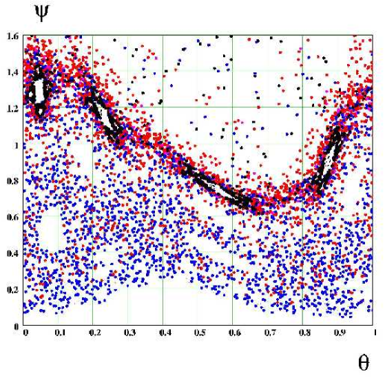
Figure 9: Phase portrait of the plasma edge, after complete destruction of the KAM surfaces. Several trajectories are chosen to represent the details of the four island remnants $q=m=4$ at a value $L=6/2\pi\sim 0.954...$ beyond the escape threshold. The plasma edge has become permeable and is strongly deformed as compared to the unperturbed circle $\psi=1$. One remarks the presence of four satellites or daughter islands around each main island.

By performing a very long iteration up to $2.10^{9\text{\ }}$time steps on a Alpha workstation, with a value $L=4.875/2\pi\sim 0.776$, we did not reach the time where the particle could possibly escape from the plasma : up to this time the trajectory remains confined by what can be considered as a KAM surface.

On the other hand, for slightly larger values of $L$ of the order of $5/2\pi\sim 0.796$, most of the magnetic lines are found to rapidly escape from the plasma (see for instance Fig.(10) for $L=5.5/2\pi\sim 0.875$). A threshold region of the stochasticity parameter has thus been found slightly below $L=5/2\pi\sim 0.796$. For larger $L$ values, magnetic lines escape across the plasma edge even when starting from the central chaotic shell.

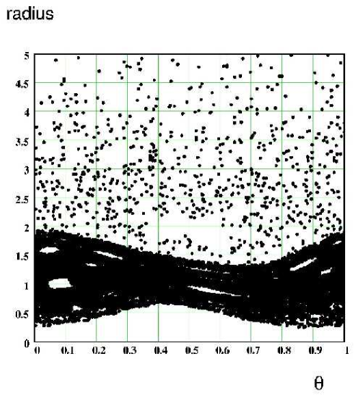
Figure 10: Single trajectory at $L=5.5/2\pi\sim 0.875$ followed during $N=16380$ iterations. After a long trapping period in the chaotic sea, this trajectory finally escapes out of the plasma edge. The initial conditions are $r=\sqrt{2\psi}=0.4$ and $\theta=0.025$.
.

3.2 Intermittent motion inside the confined plasma: crossing internal barriers

For values of $L$ smaller than this escape threshold, magnetic lines are wandering inside the plasma. We mainly consider here the case $L=4.875/2\pi\sim 0.776$ at which the edge barrier is not yet broken. We follow one single magnetic line along a large number of iterations, starting near the central region. With this value of the stochasticity parameter, the corresponding phase portrait is particularly rich, even with only one point represented every $10009$ iterations .

The chaotic sea is represented on the Fig.(11) where we recognize the protected zones corresponding to the island remnants with $q=4$, $3$, $2$ and $1$ (the central core) beside all other main rational chains.

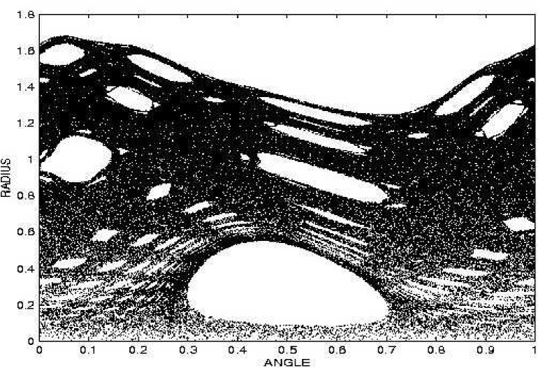
Figure 11: Phase portrait for $L=4.875/2\pi\sim 0.776$ as drawn in coordinates $\theta$ and $r=\sqrt{2\psi}$ by a single trajectory followed during $2.10^{9}$ iterations, with one point represented every $10009$ iterations. The inner shell appears slightly darker, surrounding the plasma core (white) and the magnetic axis. Long sticking occurs here around the five small $q=5/2$ islands (dark lines in the upper part of the chaotic sea).

For this trajectory the sticking stage is particularly long around the boundary of the $q=5/2$ island remnant, and lasts for several $10^{8}$ iterations. Starting from points in the neighborhood, and performing a small number of iterations ($N=16380$) we find that this dense stochastic zone takes a figure-eight form (which indicates that a period doubling has occurred) with 9 daughter islands around (see Fig.(12)). Each of the central elliptic points in these $q=5/2$ islands has already bifurcated, giving rise to an inverse hyperbolic point and to two new elliptic points.

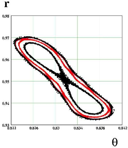
Figure 12: Detail of a small structure of the phase portrait around one of the five $q=5/2$ islands, where a long sticking stage occurs during $10^{8}$ iterations along the trajectory represented in Figs. 11 and 12.

It is most interesting to determine the time behavior of the magnetic line position in its complicated motion across the chaotic sea of  the poloidal plane. The full information has been represented on an animated movie [41]. We have followed a very long trajectory on $2.10^{9\text{\ }}$time steps starting from $\psi=0.0136125$, $\theta=0.033$. As discussed in Appendix A (Eq. (123)), this initial condition corresponds to a radius $r=0.165$ , slightly out of the central protected core of the plasma (we recall that in these notations, the edge of the plasma $\psi=1$ is at $r=\sqrt{2}$ ). From such initial conditions, the road is completely open up to the edge of the plasma, which is a resistant KAM barrier for this $L$ value, but the path is far from trivial: the magnetic line describes a path ”percolating” among the rich variety of island remnants which are known to form a hierarchical fractal structure. In that movie one remarks that the line remains for a very long ”time” in a chaotic layer, between the central protected core and some visible transport barrier ”around” $q=9/8$, and then crosses this barrier to explore the upper chaotic sea (extending up to the plasma edge). Such transitions across the barrier occur repeatedly, inward and outward, in an intermittent way and after random residence times. Shorter periods of sticking inside this barrier are also observed.

This behavior can also be represented in a $(r,t)$ graph shown in Fig.(13) where we present the time variation of the radial position : this behavior is not only stochastic, but presents different stages :

- a first period of pseudo-trapping or temporary confinement in an inner shell below $r\precsim 0.6$,

- an escape in an external shell, and a wandering stage in a wide chaotic sea, avoiding island remnants, up to $r\precsim 1.6$,

- a period of deep sticking around the five island remnants $q=5/2$ (only four bands can be seen since two of the five islands overlap in radius),

- a new wandering in the chaotic sea of the external shell, then a second stage of pseudo-trapping in the inner shell,

- and so one and so forth…

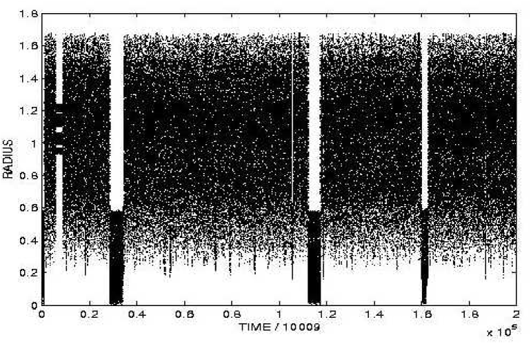
Figure 13: Radial position of a single trajectory followed during $2.10^{9}$ iterations, as function of time for $L=4.875/2\pi\sim 0.776,$with initial condition $\psi=0.0136125$, $\theta=0.033$ : different stages of trapping in different zones indicate an intermittent behaviour. Note that trapping stages are very long at may last for at least several $10^{7}$ iterations for this value of the stochasticity parameter, near the escape threshold. (Such long times near the critical threshold for large scale chaotic motion could be reminiscent of critical phenomena.

In other words the oscillating radial position of a single line is seen to wander randomly from the (inner) stochastic shell, to the stochastic sea (sometimes around $q=5/2$ island remnants) with small downward peaks indicating excursion towards and inside the transport barrier, like flood tide and ebb tide.

Such an intermittent behavior is typical of the phenomena of alternative trapping into different ”basins” of a Continuous Time Random Walk (CTRW) [42], as previously observed [43] in a stochastic layer of the Chirikov-Taylor standard map. One may wonder why these average residence times (trapping times) are so long in the present case. This could be related with the fact that the value $L=4.875/2\pi$ considered in Fig.(13) is not far from the escape threshold $L\sim 5/2\pi$, and that the latter could be the analogous of a critical point of percolation, in the vicinity of which cluster lengths and diffusion characteristic times are generally diverging as some inverse power of the deviation from the critical parameter value, with a critical exponent.

This conjecture however remains to be proved. In the present problem, such long characteristic times seem to exclude the possibility to compute the histogram (the probability distribution of these residence times), which would need awfully long iterations times in order to obtain a good statistics.

4 Localization of transport barriers

The intermittent motion described in Fig.(13) clearly exhibits intermittent periods of confined motion between structures playing the role of internal transport barriers (ITB), the most resistant curves inside the confined plasma. It is interesting to identify such barriers and to note their positions along the $q$ -profile .

4.1 Rough localization

4.1.1 Central core barrier

An initial period of pseudo trapping is observed, during which the trajectory remains in the inner shell of Fig.(11) for several $10^{6}$ iterations. This shell is separated from the protected central core of the plasma by a very strong barrier on the plasma edge which has not been crossed during $2.10^{9}$ iterations. This barrier can thus be considered as a KAM torus (or a very robust Cantorus if it could have been crossed by performing still more iterations). By analyzing the innermost points reached by the long trajectory, and performing short iteration series on several of them, we can determine which part of the trajectory is a good candidate to localize the barrier. A rational estimate of the value of the safety factor can be determined on this trajectory by carefully analyzing the (almost) periodic repetition of the variation of the poloidal angle $\theta$ in time, along with an estimation of the average poloidal rotation at each iteration, or by a direct calculation of the winding number (48) after a possible change of coordinates for innermost trajectories not encircling the origin. We find that a very rough estimate of the inner barrier protecting the plasma core from invasion from the inner shell is characterized by:

$$q_{C1}=\frac{27}{25}=1.080$$ (50)

4.1.2 Internal barrier preventing outward motion in the chaotic shell (lower Cantorus)

In this inner shell, the outward motion is limited by a series of points which has been analyzed in a similar way. Measurement of the $q$-value of the outermost trajectory in a short sample yields the following rough rational estimate:

$$q_{C2}=\frac{10}{9}=1.111$$ (51)

4.1.3 External barrier on the plasma edge

The upper edge of the chaotic sea in Fig.(11) has also been analyzed in a similar way. Iteration of some of the outermost points allows us to draw Fig.(14) which allows us to select a good candidate for the most external local trajectory. The determination of a rational approximate for its $q$-value yields:

$$q_{C4}=\frac{92}{21}=4.381$$ (52)

For this external barrier we have successively identified on Fig.(14) surfaces with $q=13/3$, $35/8$ and the outermost one : $q=92/21$. Of course a still better precision is possible, but this is enough for the present purpose.

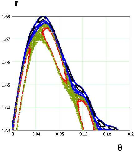
Figure 14: Structure of rational surfaces (islands) and chaotic zones below the edge KAM torus $N(4,2)$ (boundary circle) and the three convergents from below to $N(4,2$): $q=13/3$, $q=35/8$, $q=92/21$. This detailed drawing for $L=4.875/2\pi\sim 0.776$ represents short iteration times ($N=8192$), performed on the most external points selected in the long trajectory of Figs.(11 and 13). This graph reveals different structures near the plasma edge, allowing to choose the most external part of the trajectory, and a rational estimate of the $q$-value of the external barrier : a KAM surface (or a robust Cantorus).

4.1.4 Internal barrier preventing inward motion in the chaotic sea: a two-sided internal barrier (upper Cantorus)

During long intermediate stages in the intermittent history of Fig.(13), the trajectory remains above what appears as an internal barrier preventing the inner motion. A similar analysis allows us to determine a rough rational approximate for the $q$-value of the innermost part of this trajectory:

$$q_{C3}=\frac{17}{15}=1.133$$ (53)

which appear to be different from the neighboring surface $q_{C2}$ preventing upward motion from the inner shell. We are thus in presence of a two-sided transport barrier. It is quite remarkable that both sides could have been distinguished. Actually this difference clearly appears to the eyes on the movie [41] which has been realized on this simulation, in which we present a succession of snapshots to which new groups of points are added in a discontinuous way on each new picture : it can clearly be observed on some pictures how new, ”fresh” or ”recent” points are really aligned along a barrier which is different from the lower one. One of these snapshots is presented in Fig.(15).

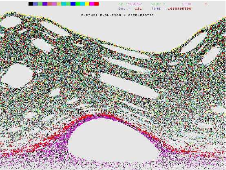
Figure 15: One of the last snapshot in the java animation. Bold points in this phase portrait $(\psi,\theta)$ represent the most recent iterated points along a single magnetic line trajectory. Here, after filling the whole chaotic sea, the line is partly confined in the chaotic shell and then is sticking around the internal barrier.

4.2 Expectations from theory of nonlinear dynamical systems

From classical theory of chaos in simple nonlinear dynamical systems [14], it is expected that the most resistant KAM torus in a $q-$interval of values is either the Golden number or at least a ”noble” number (after Percival [17]) . This is known to be the case in the standard map. When represented in a continuous fraction expansion

$$\left[a_{1},a_{2},a_{3},....,a_{j}\right]=1/\left(a_{2}+1/\left(a_{3}+1/...+1/a_{j}\right)\right)$$ (54)

the Golden number has a simple $\left[\left(1,\right)^{\infty}\right]$ coding:

$$G\equiv 1+\frac{1}{1+\frac{1}{G}}=\frac{\sqrt{5}+1}{2}=\left[1,1,1,1,......1\right]=\left[\left(1,\right)^{\infty}\right]=1.61803399....$$ (55)

and other noble numbers have a $\left(1,\right)^{\infty}$ tail, with other integers before. Most noble numbers are the ”most irrational”, defined as those with the smallest number of integers before the $\left(1,\right)^{\infty}$ tail.

In presence of magnetic shear the situation can be different: for instance, to the best of our knowledge, nobody knows why the Golden number actually plays no special role in the tokamap with monotonous $q$ -profile [16]. In other words, the special role played by the Golden KAM in the standard map does not seem to be conserved in other maps in presence of shear. We denote the most noble numbers of interest here by

$$N(i,j)\equiv\left[i,j,\left(1,\right)^{\infty}\right]=i+\frac{1}{j+\frac{1}{G}}$$ (56)

($i,j\in Z,j>1)$ which represent the ”next most irrational” numbers after the Golden one $G\equiv N(1,1).$ For $i=1$ we note that these noble numbers are ”good milestones” in the $q$ -profile since they are rather well distant, and even of measure zero [18]. It is simple to prove that the values of $N(1,j)$ are actually inserted in the $q$ -profile between successive dominant island chains $Q(j)\equiv j/(j-1)$ since it is easy to demonstrate that:

$$Q(1+j)>N(1,j)>Q(2+j)$$ (57)

Better and better rational approximants to a noble number $\omega$ (in the sense of the Diophantine approximation)  are obtained by truncating this infinite series at a higher and higher level : these rational approximants are known to converge towards the noble number $\omega$ and are called the ”convergents”, with the property ”to be the closest rational to the irrational $\omega$, compared to rationals with the same or smaller denominator” [14]. The successive convergents to an irrational number

$$\omega=\left[a_{1},a_{2},a_{3},....,a_{j,}...\right]$$ (58)

are defined by (see (54)) the series :

$$\begin{array}[]{cccccc}[a_{1}]\equiv a_{1}&\text{,}&[a_{1},a_{2}]=a_{1}+\frac{1}{a_{2}}&\text{,}&\left[a_{1},a_{2},a_{3}\right]=a_{1}+\frac{1}{a_{2}+\frac{1}{a_{3}}}&\text{,}\end{array}$$

$$\begin{array}[]{ccccc}\left[a_{1},a_{2},a_{3},a_{4}\right]&\text{,}&\left[a_{1},a_{2},a_{3},a_{4},a_{5}\right]&\text{,}&\text{etc...}\end{array}$$ (59)

When looking at the most noble $q-$values in any given interval between $q_{0}=m_{0}/n_{0}$ and $q_{1}=m_{1}/n_{1}$ (with $\left|m_{0}n_{1}-m_{1}n_{0}\right|=1$ []), it is known [44] that the most irrational number is

$$\alpha_{1}=\frac{m_{0}+G.m_{1}}{n_{0}+G.n_{1}}$$ (60)

and is expected to correspond to the most robust barrier in that interval. If we now look at the successive intervals $\left\{Q(m+1),Q(m+2)\right\}$ between the main rational chains of the dominant series $q=Q(m+1)=(m+1)/m$ (as observed in Fig.(11), we see that these intervals are Farey intervals [45] covering the real axis and the most noble $q-$values in each of these intervals are precisely given by Eq. (56) :

$$\alpha_{m}=\frac{m+1+G(m+2)}{m+G(m+1)}=1+\frac{1}{m+\frac{G}{G+1}}=1+\frac{1}{m+\frac{1}{G}}=\left[1,m,\left(1,\right)^{\infty}\right]=N(1,m)$$ (61)

(where we used $G+1=G^{2}$). These most noble numbers are not frequent and simply alternate with the main rational chains. In the barrier found ”around” $q=9/8$ the candidates for robust circles are thus $q=N(1,7)$ and $N(1,8)$ since we have $8/7>N(1,7)>9/8>N(1,8)>10/9$.

It is worth mentioning that the convergents towards these two noble numbers are, for the lower Cantorus (see the lowest approximation $10/9$ found in (51)) :

$$\frac{10}{9}\rightarrow\frac{10+9}{9+8}=\frac{19}{17}\rightarrow\frac{29}{26}\rightarrow\frac{48}{43}\rightarrow\frac{77}{69}\rightarrow\frac{125}{112},...\Rightarrow\left[1,8,\left(1,\right)^{\infty}\right]=N(1,8)=1.116<\frac{9}{8}$$ (62)

and for the upper Cantorus (see the lowest approximation $17/15$ found in (53)) :

$$\frac{9}{8}\rightarrow\frac{9+8}{8+7}=\frac{17}{15}\rightarrow\frac{26}{23}\rightarrow\frac{43}{38}\rightarrow\frac{69}{61}\rightarrow\frac{112}{99},...\Rightarrow\left[1,7,\left(1,\right)^{\infty}\right]=N(1,7)=1.131<\frac{8}{7}$$ (63)

where successive approximants are alternatively from below and from above, due to the $\left(1,\right)^{\infty}$ series in the Farey coding [45], see Fig.(16).

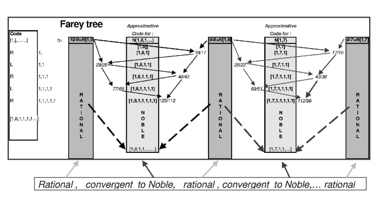
Figure 16: Farey tree indicating how the most noble number in a given interval between rationals ($10/9$ and $9/8$, or $9/8$ and $8/7$) can be built with results $N(1,8)$ or $N(1,7)$.

It is well known that the numerators and denominators $p_{\mu}$ of the successive approximants actually grow as a Fibonacci series $p_{\mu+2}=p_{\mu+1}+p_{\mu}$, with an asymptotic growth rate $\lim_{\lambda\rightarrow\infty}$ $p_{\mu+1}/p_{\mu}=G$ given by the golden number $G$.

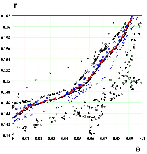
Figure 17: The upper Cantorus for $L=4.875/2\pi$ can be localized in the central region, between bold dots. Here we have plotted series of $2046$ iterations along each of the island chains with rational $q$ values corresponding to the following approximants to the upper Cantorus $N(1,7)$ : $q=17/15$, $43/38$ and $112/99$ from above, and $q=9/8$, $26/23$ and $69/61$ from below.

In Fig.(17), we have plotted a series of $2046$ iterations along the island chains with rational $q$-values corresponding to the following approximants to the upper Cantorus (63) : $q=17/15$, $43/38$ and $112/99$ from above, and $q=9/8$, $26/23$ and $69/61$ from below. This allows us to localize the upper Cantorus on this graph as being located in the very thin interval located between bold dots.

4.3 Identification of ”convergents” towards these most noble Cantori

It is simple but numerically delicate to check that the barrier is composed of two Cantori localized precisely on these two most noble numbers : a lower Cantorus on $N(1,8)$ and an upper Cantorus on $N(1,7)$. Why are the most resistant KAM tori located around $q=9/8$ for this value of $L$ could probably not be deduced on theoretical grounds. Of course, beside the most robust barrier described here, other, less robust barriers also exist. A detailed analysis of the various thin downward peaks in Fig.(13) reveals that the lower boundary of the magnetic line motion in the stochastic sea is actually oscillating in time, and does not always correspond to the same upper Cantorus above the island chain $q=9/8$ as defined in Eq. (63). The lower boundary of the stochastic sea can be found on different Cantori located most often above the island chain $q=6/5$, but also on the Cantori above $q=7/6$ and $8/5.$ This seems to indicate that a global barrier could rather be composed of different sticking regions around island chains with main rational $q-$values, and that these sticking regions are limited successively by the Cantori between them, in some kind of cascading process. Global motion in these boundary regions could then be described [41] as a succession of approaches, like flood tide and ebb tide, allowing the magnetic line to pass through the successive barriers.

During the upward motion starting from the chaotic layer, the most important barrier (but not the last one) nevertheless remains the upper Cantorus $q=N(1,7)$ above the islands $q=9/8$ : once this one has been passed, the magnetic line rapidly invades the whole chaotic sea. As seen in Fig.(13), the inverse, downward motion from the chaotic sea however encounters several barrier crossing, back and forth, before crossing the upper Cantorus and entering in the zone between the two Cantori composing the ITB described in this paper.

4.3.1 Convergent island chains towards the two Cantori

Localization of island chains with given $q-$value can be obtained numerically with great precision by searching hyperbolic and/or elliptic periodic points, by a numerical algorithm derived from a generalization of the Fletcher-Reeves method, involving the Jacobi matrix of the tokamap, explained in Appendix B. Localizing the position of a noble Cantorus can only be achieved as a limiting procedure, by localizing the series of its convergents, as given by Eqs. (62, 63).

In order to check the above predictions we have sampled (in a very long trajectory of $2.10^{9}$ iterations) various sections of trajectory (a) reaching the highest $\psi-$values in the chaotic shell (below the lower Cantorus), and (b) reaching the lowest $\psi-$values in the chaotic sea (above the upper Cantorus): such trajectories remain indeed well separated, by the width of the barrier. Then we have checked that any of these sections of trajectory (a) remains indeed below the limit of convergence of $N(1,8)$ of the lower Cantorus, more precisely below the limit of the convergents from below :

$$\begin{array}[]{ccc}\frac{10}{9},\frac{29}{26},\frac{77}{69},\frac{202}{181},\frac{529}{474},\frac{1385}{1241},...\Rightarrow N(1,8)&&\text{(from below)}\end{array}$$ (64)

and that any of these sections of trajectory (b) remains indeed above the limit of convergence of $N(1,7)$ of the upper Cantorus, more precisely above the limit of the convergents from above :

$$\begin{array}[]{ccc}\frac{17}{15},\frac{43}{38},\frac{112}{99},\frac{293}{259},\frac{767}{678},\frac{2008}{1775}...\Rightarrow N(1,7)&&\text{(from above)}\end{array}$$ (65)

In other words we have checked that observed trajectories in the chaotic shell and in the chaotic sea remain actually always on their own side of the pair of Cantori, which localizes the barrier.

4.3.2 Convergent island chains towards noble KAM’s on the edge and around the plasma core

By the same method we have also identified the $q-$value of the robust boundary circle forming the plasma edge as being equal to $N(4,2)$ which appears to be the most irrational between $q=4$ and $q=4.5$, according to Eq. (60) :

$$\frac{4}{1}\rightarrow\frac{4+9}{1+2}=\frac{13}{3}\rightarrow\frac{22}{5}\rightarrow\frac{35}{8}\rightarrow\frac{57}{13}\rightarrow\frac{92}{21}\rightarrow\frac{149}{34},...\Rightarrow$$

$$\left[4,2,\left(1,\right)^{\infty}\right]=N(4,2)=4.381<\frac{9}{2}$$ (66)

in agreement with (52). There should probably exist a stronger barrier out of the ”plasma edge” on $N(4,1)\sim 4.618,$ but this one remains out of reach for trajectories starting from the plasma bulk at the considered value $L=4.875/2\pi$ since the KAM on the edge at $q=N(4.2)<N(4,1)$ has not yet been broken.

We have also identified the $q-$value of the robust boundary circle protecting the plasma core as being equal to $N(1,11)$, the most irrational between $q=1$ and $q=12/11$, according to Eq. (60):

$$\frac{1}{1}\rightarrow\frac{1+12}{1+11}=\frac{13}{12}\rightarrow\frac{25}{23}\rightarrow\frac{38}{35}\rightarrow\frac{63}{58}\rightarrow\frac{101}{93},...\Rightarrow$$

$$\Rightarrow\left[1,11,\left(1,\right)^{\infty}\right]=N(1,11)=1.086<\frac{12}{11}$$ (67)

which is in poor agreement with the above rapid estimate (50), but correct to the first three digits.

4.3.3 The ITB: a double sided barrier around $q=9/8$

The final scheme which results from the above measurements on a very long tokamap trajectory at $L=4.875/2\pi$ is the following. A magnetic line with an initial condition inside the inner shell (IS) actually has an inward motion limited by a robust KAM torus protecting the plasma core (or a Cantorus ?) at

$$q_{IS}>N(1,11)=1.086>\frac{13}{12}$$ (68)

and an outward motion limited by a semi-permeable Cantorus at:

$$q_{IS}<N(1,8)=1.116$$ (69)

This numerical analysis shows that noble Cantori are good candidates to be identified with internal transport barriers, as could have been anticipated from the relation between KAM theory and number theory [18].

Once arrived in the main chaotic sea (CS) extending up to the plasma edge, the magnetic line wanders around island remnants, remains stuck around some of them (here in Figs.(13, 11) around the $q=5/2$ chain), but its inward motion is limited by a semi-permeable Cantorus

$$q_{CS}>N(1,7)=1.131>\frac{9}{8}$$ (70)

The measurements indicate that this inward-motion limit in the chaotic sea is different from (and located above) the outward motion limit of the IS :

$$N(1,8)=1.116<\frac{9}{8}=1.125<N(1,7)=1.131$$ (71)

We have thus observed the existence of a two-sided transport barrier around $q=9/8$ and limited on each side by a Cantorus, respectively at $q=N(1,8)$ and $q=N(1,7)$.

On the other end, the outward motion in the chaotic sea is limited by a curve which will be proved in Section (5) to be a KAM surface at

$$q_{CS}<N(4,2)=4.382$$ (72)

which is the most irrational number between $4$ and $4.5$. This external KAM surface thus appears indeed a good candidate for the external barrier observed here.

We are thus in presence of a double-sided transport barrier, composed of two Cantori, the lower Cantorus with noble $q-$value $N(1,8)=1.116$, the upper Cantorus with noble value $N(1,7)=1.131.$ These Cantori appear on Fig.(21). From (57) we have $N(1,7)>Q(9)>N(1,8)$ , which shows that the rational surface $q=Q(9)=9/8$ is actually between these two Cantori and thus inside the transport barrier. In this sense, one can say that this internal transport barrier is actually located around a dominant rational surface, in spite of the fact that it is actually composed of two irrational, noble Cantori.

4.3.4 Experimental localization of barriers in the Tokamak $q$ -profile

From the experimental point of view, transport barriers in tokamaks are indeed generally observed ”around” the main rational $q$-values [2].

In the RTP tokamak, with a wide range of $q$-values ($0.8\Longrightarrow 5$) in a reversed sheared profile, it has been observed, by varying the heat deposition radius $\rho_{dep}$ of off-axis ECH heating, that the central electron temperature $T_{e}(0)$ decreases by a series of plateaux [2]. It is observed that the values of  $q_{m}$ of the different plateaux fall in half-integer bands, i.e. $q_{m}$ crosses a half-integer value each time the discharge transits from one plateau to the next. Since these transitions correspond to the loss of a TB, these authors deduced that ”the barriers are associated with half-integer values of $q$ .”

It has been reported that some ”ears” appear in the $T_{e}$ profile (appearance of one bump on each side of the central value) when the heat deposition radius $\rho_{dep}$ is localized inside a transition between two plateaux [2]. We note that the existence of such ”ears” could be an indication in favor of the existence of a double-sided semi-permeable TB around $\rho_{dep},$ as found in the previous Section (4.3.3). Such ”ears” appear to be unstable and to crash in a repetitive fashion, showing that the barrier can indeed be crossed and appears to be permeable.

The central sawteeth allows to place the first barrier ”near” $q=1$ ; off-axis sawteeth indicate other barriers near $q=3/2$, $2$ and $3$. Remaining barriers are attributed to $q=4/3$ and $5/2$.

In all cases the barriers observed in experiments are associated with those ”dominant rational” $q$-values, but a specific experimental work could hardly have been done in order to determine more precisely the possible role of noble or other irrational values around these ”dominant rationals”.

Up to now it has been generally admitted [2], [8], [10] that internal transport barriers could correspond to rational $q$-values, where primary island appear. Chaotic motion can be observed between these primary rational islands but mainly around the hyperbolic points. The picture we obtain here is rather different. It is well known that, in presence of several island chains, secondary islands appear and accumulate around irrational surfaces where KAM surfaces finally broke themselves into discrete pieces forming a Cantorus. This is precisely the location where we have found internal barriers: they appear as Cantori on irrational surfaces rather than rational surfaces.

This finding can in turn be helpful to build transport models like the $q$-comb model [23], [24]. From experimental considerations, such models define indeed barriers are localized around main rational $q$-values, but the width if the barriers has still to be defined. We propose to localize the edges of each barrier on the most irrational value in the prescribed domain.

4.4 Last barrier in the standard map: the golden KAM

In order to illustrate the destruction of a robust barrier, there exists one example in which a KAM surface can be represented just at the critical point where it is broken into a Cantorus. This is the case of the standard map [27] where the critical value of the stochasticity parameter is known with a very high precision. It is interesting to remind that the last KAM surface in that case has been identified to be the Golden KAM with $q$-value equal to $G$, the golden number. The breaking of this surface and its transformation into a Cantorus is known to occur at a critical value of the stochasticity parameter which is known [18] to be given by $K=K_{C}=0.971635406$. Because such a drawing is not easily found in the literature for this value of $K$, it appears worthwhile to present the trajectory following this critical curve. In Fig.(18) we present part of the phase portrait of the standard map for $K=K_{C}$. Two series of islands remnants $q=8/5$ and $q=5/3$ can  be seen, corresponding to two convergents towards the Golden number $G=\lim$ $of\left(\frac{3}{2},\frac{5}{3},\frac{8}{5},\frac{13}{8},...\right)$.  The last KAM with $q=G$ is exhibited inbetween, and it appears as the last existing non-chaotized KAM surface, surrounded by chaotic layers around rational islands.

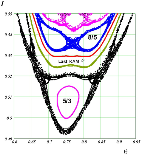
Figure 18: Part of the phase portrait of the standard map for $K=K_{C}$. Two series of islands $q=8/5$ and $q=5/3$ can  be seen, corresponding to two convergents towards the Golden number $G$.  The last KAM with $q=G$ is exhibited inbetween, and it appears as the last existing non-chaotized KAM surface; its initial conditions are $I=0.52969$, $\theta=0.75$.

This example shows the detailed structure of an irrational KAM barrier surrounded by chaotic, permeable zones.

4.5 Perturbed $q$ -profile in the tokamap

4.5.1 Exact perturbed $q$-profile

In order to understand the radial positions of these barriers on the exact $q$ -profile of the tokamap, we have succeeded to draw a one-dimensional $q$-profile of the magnetic surfaces, not as function of the radius (since perturbed surfaces are not circular anymore), but as function of the distance $X$  between the polar axis and their intersection point in the equatorial plane. We have calculated the intersections of several trajectories with the equatorial plane (at $\theta=0$ and $\theta=0.5$) and measured their $q$-value, by computing the average increase of the poloidal angle according to Eq.(48).

In this way we obtain a rather precise profile of the perturbed $q$-values of various magnetic surfaces or island chains, represented at the two (non-symmetrical) points where they cross the equatorial plane, see Fig.(19). Let us recall that the radius $r$ represented on the various figures is defined by $r=\sqrt{2\psi}$ (see Eq.(36). This variable $r$ varies from $0$ to $\sqrt{2}$ on the edge of the plasma, while the variable $x=\sqrt{\psi}=r/\sqrt{2}$ varies from $0$ to $1$ and represents the reduced radial coordinate with respect to the small radius of the torus.

$$x=\sqrt{\psi}=r/\sqrt{2}$$ (73)

The abscissa in Fig.(19) is represented between $X\equiv x$ $cos\theta=1$ on the weak field side and $X=-1$ on the strong field side, as compared with the unperturbed imposed $q$ -profile (Eq. (39)).

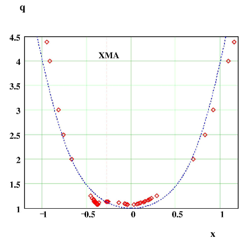
Figure 19: Calculated points (diamonds) of the perturbed $q$-profile (around the magnetic axis) in the equatorial plane for $L=4.875/2\pi\sim 0.776$, with the plasma extending from $X=-1$ to $+1$, showing overall agreement with the unperturbed profile (dotted line), except for the the appearance of a local maximum on the magnetic axis (XMA).

The measured points roughly agree with the unperturbed curve (Fig.(19)). But a detailed drawing in Fig.(20) reveals a rather unexpected point: the perturbed safety factor profile in the equatorial plane exhibits a local maximum on the magnetic axis, and a minimum on both sides.

The measured $q$-value near the magnetic axis appears to be

$$q_{MA}\simeq 1.1346\succsim\frac{17}{15}$$ (74)

This non-monotonous perturbed $q$ -profile , which is spontaneously created by the magnetic perturbation, could be the reason for the appearance of transport barriers in the tokamap.

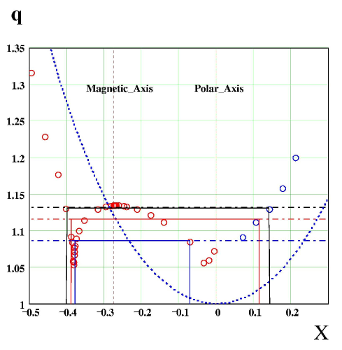
Figure 20: Detail of the perturbed $q$-profile (measured around the magnetic axis) in the equatorial plane (circles) for $L=4.875/2\pi\sim 0.776$, as compared with the unperturbed profile (dotted line), showing the appearance of a local maximum on the magnetic axis, and of two minima. Horizontal levels represent (from top to botom) the $q$-values $N(1,7)=1.131$ of the upper Cantorus (which corresponds approximately to the higher $q$-values of the bump), $N(1,8)=1.116$ of the lower Cantorus, and $N(1,11)=1.086$ of the KAM barrier protecting the plasma core, along with the extension of these curves with the equatorial axis $X$. The value on the magnetic axis is $q_{MA}=1.1346>N(1,7)$ and lies at the center of a profile which is locally hollow at very small distances from the magnetic axis (not visible at this scale)

4.5.2 An ITB in the rev-tokamap

Transport barriers are very frequent in reversed shear situations, and they also appear in the tokamap model for such cases. We recall indeed that a transport barrier has already been shown to occur around the minimum of a reversed shear $q$ -profile (”revtokamap” [37]). In the discussion of Fig. 4 in Ref. [37], for $L=2.8/2\pi$, it is observed that ”the chaotic region is sharply bounded from below by a KAM barrier” located at $1/q=0.5772$. We note that this value is only $0.5\%$ away from a noble value $1/q=0.5802$ which corresponds to $q=[1,1,2,\left(1,\right)^{\infty}]$ $=1+\left(1/\left(1+1/\left(2+1/G\right)\right)\right)$ $=1.7236068...$ which is larger than the Golden number and appears from (60) to be the most irrational number between $5/3$ and $7/4$. Within a precision of $0.5\%$, the transport barrier found in [37] could thus well be located on a noble value again, even in the previous situation of a reversed magnetic shear profile.

4.5.3 Inverse shear in the tokamap

The inner shell, which has been observed between $q_{C1}=1.080$ and $q_{C2}=1.111,$ actually involves $q$-values lower than that measured on the magnetic axis (Eq. (74)), down to $q\simeq 1.07$ (see Fig.(20), precisely because of the non-monotonous profile.

One can see that the $q$-values decrease from the magnetic axis towards a separatrix passing through the polar axis (on which two hyperbolic points are superposed, as long as $L<1$). This whole region inside the separatrix would appear however to have $q=1$ if and only if  $q$ was computed around the polar (geometrical) axis, but this way of counting has not much physical meaning, besides showing that this plasma core could appear as an island $m=n=1$ in the reference frame of the polar axis. As a result, trajectories inside the chaotic shell have actually $q-$values (around the magnetic axis) which decrease from the boundary circle for those trajectories which do not enclose the polar axis $(\psi=0,\theta=0)$, but which increase for those which encircle the polar axis, up to the value $N(1,8)$ of the lower Cantorus. In the chaotic sea, the $q$ -profile is monotonously growing : trajectories have $q-$values higher than the upper Cantorus and lower than the boundary circle on the edge, which is the expected situation.

In summary, starting from the magnetic axis, we first find a regular zone, with a decreasing perturbed $q$ -profile away from the magnetic axis (where $q_{MA}\simeq$ $1.13461$), then a robust boundary circle located on $q=N(1,11)$ protecting the regular plasma core, then decreasing $q-$values up to the separatrix, then a regular increase of the $q$ -profile with a $q=10/9$ rational chain, a lower semi-permeable lower Cantorus on $q=N(1,8)$, the island remnants $q=9/8$, then the upper Cantorus on $q=N(1,7)$ below the rational chain $q=8/7$, etc… up to the robust KAM torus on the edge at $N(4,2).$ The two robust barriers and the two Cantori are represented on Fig.(21) along with a part of each chaotic region.

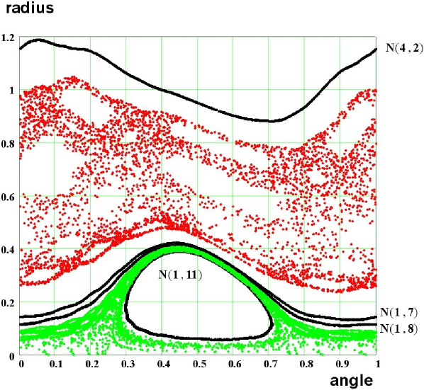
Figure 21: The main noble transport barriers are represented in bold lines in normalized coordinates: ”radius”= $x=\rho/a=\sqrt{\psi}$ and ”angle”= $\theta$. The robust KAM $N(1,11)$ separating the central protected plasma core (in white) from the chaotic shell. The two semi-permeable Cantori $N(1,8)$ and $N(1,7)$ form an internal barrier resulting in a very slow and intermittent motion towards the chaotic sea. The robust KAM torus on the plasma edge $N(4,2)$ has been identified to have a vanishing flux.

4.6 Sticking measurements

On the other hand, we have seen in Fig.(13) that a long trapping stage is observed in the chaotic zone surrounding the island remnants $q=5/2$. For a much longer trajectory ($10^{11}$ iterations) one observes that such temporary but long trapping can occur around almost all rational and specially around the main islands known to play a role in the tokamaks: $q=2/1$, $5/2$ and $3/1$. In Fig.(22) we have computed the normalized histogram showing the occurrence $H$ of sticking times longer than $10^{5}$ (in a run of $10^{11}$ iterations with $L=4.875/2\pi$), obtained by a sliding average, as a function of the radial position $\psi$ of the visited island chain. The values of $\psi$ are taken within small intervals of $2.10^{-4}$.  This graph exhibits the frequent occurrence of long sticking times in and around the main rational chains : the two bumps correspond to widespread $\psi$ values of a line wandering in the chaotic shell (around $\psi\sim 0.1$) and in the chaotic sea (around $\psi\sim 0.4$ to $0.8$). These are the main two chaotic zones. On the other hand one remarks sharp peaks representing long sticking events at the corresponding $\psi$ values. In the chaotic sea bump, we identified very precisely (by measuring the exact average-$\psi$ value of the corresponding $q$) long and frequent sticking events around island remnants $q=2$, $5/2$ and $3$ (with satellite peaks at neighboring rationals), etc… This kind of graph yields a precise measurement of the richness of trapping phenomena.

Figure 22: Normalized histogram showing the occurrence $H$ of sticking times longer than $10^{5}$ (in a run of $10^{11}$ iterations with $L=4.875/2\pi$), obtained by a sliding average, as function of the radial position $\psi$ of the visited island chain. The values of $\psi$ are taken within small intervals of $2.10^{-4}$.  This graph exhibits the frequent occurrence of long sticking times in and around the main rational chains  : the two bumps correspond to widespread $\psi$ values of a line wandering in the main two chaotic zones: the chaotic shell (around $\psi\sim 0.1$) and in the chaotic sea (around $\psi\sim 0.4$ to $0.8$).

It would be interesting to study the characteristics of the other secondary barriers, surrounding the ”holes” in the phase portrait Fig.(11) and to determine if such local barriers also correspond to noble Cantori in the profile of the local $q$-value (around the local magnetic axis in the center of the island remnant). For instance a sticking region is easy to observe along the edge on the $q=9/8$ islands.

The interest of this new description of ITB’s in tokamaks is that mathematical tools exist for the description of the motion across such Cantori (”turnstiles” etc… [46]), and these tools can be used to study transport across internal transport barriers in confined plasmas. Calculation of the flux through a Cantorus, defined by the limit of its convergents, can be performed by using the turnstile mechanism [46]. This subject is presented in the next Section 5.

5 Calculation of the flux across noble barriers

The study of a single long orbit points out some transport phenomena which occur between some phase-space’s zones separated by internal transport barriers (ITB), but it does not give information about the flux through these barriers ( i.e. the area of the set formed by points which pass through a ITB at every iteration). This information will be obtained in this section from Mather’s theorem. Using Greene’s conjecture we confirm the observed existence, for $L=\frac{4.875}{2\pi}\sim 0.776$, of the invariant circle on the plasma edge having the rotation number $\omega_{1}=\frac{1}{N(4,2)}$ and of a Cantorus having the rotation number $\omega_{2}=\frac{1}{N(1,7)}.$  Both Greene’s and Mather’s approaches use the intimate connection between quasiperiodic and periodic orbits.

5.1 Periodic and quasiperiodic orbits. The action principle

Let us remind some definitions and useful basic results in the theory of dynamical systems.

The”lift” of the map $T:[0,1)\times\mathbf{R\rightarrow}[0,1)\times\mathbf{R}$, $T\left(\theta,\psi\right)=\left(\theta^{\prime}\left(\mathop{\mathrm{m}od}1\right),\psi^{\prime}\right)$ is the application $\overline{T}:\mathbf{R\times R\rightarrow R}$ defined by $\overline{T}\left(\theta,\psi\right)=\left(\theta^{\prime},\psi^{\prime}\right)$ (because the $\left(\mathop{\mathrm{m}od}1\right)$ is not applied for $\theta^{\prime}$, the lift $\overline{T}$ allows to take into account the number of turns along $\theta$).

The map $T$ $:[0,1)\times\mathbf{R\rightarrow}[0,1)\times\mathbf{R}$ is called a twist map if $\frac{\partial\theta^{\prime}\left(\theta,\psi\right)}{\partial\psi}\neq 0$ for all $\left(\theta,\psi\right)\in[0,1)\times\mathbf{R}$. It is a left (respectively right) twist map if $\frac{\partial\theta^{\prime}\left(\theta,\psi\right)}{\partial\psi}<0$ (respectively $\frac{\partial\theta^{\prime}\left(\theta,\psi\right)}{\partial\psi}>0$) for all $\left(\theta,\psi\right)\in[0,1)\times\mathbf{R}$, which means that the perturbed winding number is a monotonously decreasing (respectively increasing) function of $\psi$.

A point $\left(\theta_{0},\psi_{0}\right)$ is a periodic point of type $\left(n,m\right)$, with periodicity $m$, if $\overline{T}^{m}\left(\theta_{0},\psi_{0}\right)$ $=\left(\theta_{0}+n,\psi_{0}\right)$. The rotation number of a periodic orbit exists and is equal to $\iota/2\pi=n/m$ (i.e. the limit in Eq.(48) exists); it is clearly independent of the initial point on a periodic chain. This global property persists for invariant curve, under some restriction on the map. The rotation number may also be irrational in this case. Beside periodic orbits and invariant curves (called invariant circles, for topological reasons), an intermediate case of invariant set exists, on which rotation number exists and is irrational: the Cantori. The dynamics on these three types of invariant set is generally quasiperiodic: the ”time” dependence can be expressed by a generalized Fourier series, with rational frequencies for rational $\omega$, and irrational incommensurate frequencies in the remaining cases (see Ref. [47] or Ref. [48] for details). Both periodic and quasiperiodic points can be obtained as stationary points in the action principle.

The ”action principle” for maps is the analogous of the Lagrangian variational principle in continuous dynamics. In the case of Hamiltonian twist maps, the action generating function $F_{a}$ (defined in Section (2.2)) plays the role of a Lagrangian for discrete systems.

Theorem 1

(action principle for periodic orbits) Let $T:S^{1}\times\mathbf{R\rightarrow S}^{1}\times\mathbf{R}$ be an area preserving twist map , $F_{a}:\mathbf{R}\times\mathbf{R}\rightarrow\mathbf{R}$, its action generating function and $\left\{\left(\theta_{0}^{\ast},\psi_{0}^{\ast}\right),...,\left(\theta_{m-1}^{\ast},\psi_{m-1}^{\ast}\right)\right\}$ a periodic orbit of $T$ of period $m$. Then $\left\{\theta_{0}^{\ast},...,\theta_{m-1}^{\ast}\right\}$ is a stationary point of the action

$$\mathcal{A}\left(\theta_{0},...,\theta_{m-1}\right)=F_{a}\left(\theta_{0},\theta_{1}\right)+F_{a}\left(\theta_{1},\theta_{2}\right)+...+F_{a}\left(\theta_{m-1},\theta_{0}\right)$$ (75)

A very simple proof is presented in Ref. [49]

In 1927 Birkhoff [50] showed that every area-preserving twist map has at least two periodical orbits of type $\left(n,m\right)$ for each rational winding number $\frac{1}{q}=\frac{n}{m}$ in an appropriate interval (called the twist interval). For area-preserving twist map it can be proved (see Ref. [47]  p.38 for commentaries) that, for each rational $\frac{n}{m}$ in the twist interval described by the map, there exists at least one periodic orbit of type $\left(n,m\right)$ which extremizes $\mathcal{A}$ (it is called extremizing orbit) and at least one periodic orbit of type $\left(n,m\right)$ which is a saddle point of $\mathcal{A}$ (it is called a maxmin orbit).

In order to study the linear stability properties of a $\left(n,m\right)$- periodic orbit one computes the multipliers of the orbit (i.e. the eigenvalues $\lambda$ and $\frac{1}{\lambda}$ of the Jacobi matrix associated to $\underset{m\,\,-\,\,times}{\underbrace{T\circ T\circ....\circ T}}$ in an arbitrary point of the orbit) or the residue

$$R=\frac{2-\lambda-1/\lambda}{4}$$ (76)

If $R<0$ (i.e. $\lambda>0$ , $\frac{1}{\lambda}>0$) the orbit is formed by direct hyperbolic points (which are unstable). If $R\in\left(0,1\right)$ (i.e. $\lambda$ and $\frac{1}{\lambda}$ are complex conjugate numbers and $\left|\lambda\right|=\left|\frac{1}{\lambda}\right|=1$) the orbit is formed by elliptic points (which are stable). If $R>1$ (i.e. $\lambda<0$, $\frac{1}{\lambda}<0$) the orbit is formed by inverse hyperbolic points (which are unstable).

In Ref. [51] it was proved that every extremizing orbit has negative residue and that every maxmin orbit has a positive residue. It results that every extremizing orbit is formed by direct hyperbolic points and the maxmin orbit is formed by elliptic points (if $R\in\left(0,1\right)$) or by inverse hyperbolic points (if $\ R>1$).

The action principle for quasiperiodic orbits was proposed by Percival (in Ref. [52]). In 1920 Birkhoff proved that any quasiperiodic orbit is the graph of a function (see Ref. [53]). It can be written in the form

$$\left\{\left(\theta\left(t\right),\psi(t)\right),\,\,t\in\mathbf{R}\right\}$$ (77)

where $\theta:\mathbf{R\rightarrow R}$ is an increasing function having the periodicity property $\theta\left(t+1\right)=\theta\left(t\right)+1$ for all $t\in\mathbf{R}$, and where

$$\psi(t)=-\frac{\partial F_{a}}{\partial\theta}\left[\theta\left(t\right),\theta\left(t+\omega\right)\right]$$ (78)

In these terms the action principle can be written as follows.

Theorem 2

( the action principle for quasiperiodic orbits) Let $T:S^{1}\times\mathbf{R\rightarrow S}^{1}\times\mathbf{R}$ be an area preserving twist map, $F_{a}:\mathbf{R}^{1}\times\mathbf{R}^{1}\rightarrow\mathbf{R}$ its action generating function, $\omega\in\left(0,1\right)$ an irrational number and $\left\{\left(\theta\left(t\right),\psi\left(t\right)\right)\;\;/\;\;t\in\mathbf{R}\right\}$ a quasiperiodic orbit having the rotation number $\omega.$ Then $\theta$ is a stationary point of the functional

$$\mathcal{A}\left(\theta\right)=\overset{1}{\underset{0}{\int}}F_{a}\left[\theta\left(t\right),\theta(t)+\omega\right]\text{ }dt$$ (79)

For twist maps, Mather (see Refs. [54] and [55]) proved the existence of a stationary and moreover ”extremizing” function $\theta_{ext}$ which extremizes the functional $\mathcal{A}$ (79). It gives rise to an invariant set $\left(C\right)$. Its equation can be obtained from (77, 78). If $\theta_{\text{ext}}$ is continuous then $\left(C\right)$ is an invariant circle. If $\theta_{\text{ext}}$ is not continuous (but has a countable set of discontinuities because it is monotonous), then the closure (the set of the limit points) of $\left(C\right)$ would be a Cantor set, called ”Cantorus”. A very good survey on this problem is given in Ref. [47].

5.2 Study of quasiperiodic orbits via periodic orbits

The invariant set (invariant circle or Cantorus) having the irrational rotation number $\omega$ was obtained using a stationary point $\theta_{ext}$ of the action functional $\mathcal{A}\left(\theta\right)$ defined in (79), but it is also the limit circle of a sequence of periodic orbits having rotation numbers $\frac{n_{\nu}}{m_{\nu}}$ , when $\underset{\nu\rightarrow\infty}{\lim}\frac{n_{\nu}}{m_{\nu}}=\omega.$ High order periodic orbits may thus be considered as good enough approximations for the invariant set and the study of their properties gives information about the invariant set properties. So, an irrational magnetic surface can be described as the limit of its rational convergents by observing higher and higher order periodic motions.

There are at least two approaches to study the connection between these invariant sets and the periodic orbits: the Greene’s conjecture (which relates the existence of the invariant set to the stability of a particular sequence of periodic orbits) and the Mather’s theorem (which gives necessary and sufficient conditions for the existence of the invariant set and computes the flux through it).

For a noble number $\omega$ we will denote by $\left(\frac{n_{\nu}}{m_{\nu}}\right)_{\nu\in\mathbf{N}}$ the sequence of its convergents (see Sections 4.2 and 4.3 for definitions and computations). We denote by $R_{\nu}^{+}$ the residue of a maxmin orbit (passing through elliptic or inverse hyperbolic points) and $R_{\nu}^{-}$ the residue of an extremizing orbit (passing through direct hyperbolic points) of type $\left(n_{\nu},m_{\nu}\right)$.

Greene’s conjecture (in Refs. [56] and [57]) predicts that there would be three situations:

- subcritical ( $R_{\nu}^{+}\rightarrow 0$ and $R_{\nu}^{-}\rightarrow 0$ ); in this case there is sequence of island chains converging to a smooth invariant circle having the rotation number $\omega$.

- critical ( $R_{\nu}^{+}\nrightarrow 0$ and $R_{\nu}^{-}\nrightarrow 0$ but they are bounded in $\left(0,\infty\right)$ and in $\left(-\infty,0\right)$), respectively; in this case there is a sequence of island chains converging to a non smooth invariant circle having the rotation number $\omega$.

- supercritical ( $R_{\nu}^{+}\rightarrow\infty$ and $R_{\nu}^{-}\rightarrow-\infty$); in this case there is no invariant circle having the rotation number $\omega$, but there is a Cantorus  with this rotation number $\omega$.

In Ref. [58] a partial proof is presented, but the conjecture is not yet completely proved.

On the other hand, in Ref. [59] Mather gives an equivalent condition to the existence of an invariant circle having the rotation number $\omega$. For a left twist map and a rational $\frac{n}{m}$ in the twist interval one can define

$$\Delta\mathcal{A}_{n/m}=\mathcal{A}_{\text{extremizing}}-\mathcal{A}_{\text{maxmin}}$$ (80)

the difference of action $\mathcal{A}$  between the extremizing orbit and the maxmin orbit of type $\left(n,m\right).$ In (80) $\left|\Delta\mathcal{A}_{n/m}\right|\$ is the escape area from a domain bounded by an arbitrary curve $\left(C\right)$ passing by the $m$ points of the maxmin orbit and by the $m$ points of the extremizing orbit of type $\left(n,m\right).$Let us remind that the escape area  (the flux) from the domain $R_{(C)}$ bounded by the closed curve $\left(C\right)$, under the map $T$, is defined by

$$L\left(R_{C},T\right)\overset{def}{=}Area\left(T\left(R_{C}\right)-R_{C}\right)$$ (81)

In Ref.[46] a very interesting result is proved for right twist maps. It can be easily adapted for the twist maps as follows. If $\left(C\right)\cap T\left(C\right)$ consists in $2m$ points of an extremizing orbit and of a maxmin orbit of type $\left(n,m\right)$ then  

$$L\left(R_{C},T\right) = \left|\overset{m-1}{\underset{j=0}{\sum}}\left(F_{a}\left(\theta_{j}^{\left(u\right)},\theta_{j+1}^{\left(u\right)}\right)-F_{a}\left(\theta_{j}^{\left(s\right)},\theta_{j+1}^{\left(s\right)}\right)\right)\right|=\text{ \ \ \ \ \ \ \ \ \ \ \ \ \ \ }$$ (82)

$$\left|\mathcal{A}_{\text{extremizing}}-\mathcal{A}_{\text{maxmin}}\right| = \left|\Delta\mathcal{A}_{n/m}\right|$$ (83)

In this formula, $\left(\theta_{j}^{\left(u\right)},\psi_{j}^{\left(u\right)}\right)$ and $\left(\theta_{j}^{\left(s\right)},\psi_{j}^{\left(s\right)}\right)$, for $j\in\left\{1,2,...,m\right\}$, are the points of the extremizing orbit and (respectively) of the maxmin orbit of type $\left(n,m\right)$. An example with periodicity $m=3$ is illustrated in Fig (23).

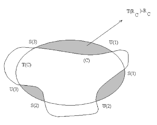
Figure 23: The figure visualizes the escape area from a bounded domain. The curve $T(C)$ is the image of the closed curve $(C)$ after one iteration by the map $T$ . The domain $R_{C}$ is the domain bounded by $(C)$. The set $T(C)\cap(C)$ consists in three unstable periodic points (namely $U(1)$, $U(2)$ and $U(3)$) and in three stable points (namely $S(1)$, $S(2)$ and $S(3)$).

Mather’s theorem states that there is an invariant circle having the rotation number $\omega$ if and only if $\underset{\nu\rightarrow\infty}{\lim}\Delta\mathcal{A}_{n_{\nu}/m_{\nu}}=0$. Otherwise, the sequence $\left(\Delta\mathcal{A}_{n_{\nu}/m_{\nu}}\right)_{\nu\in\mathbf{N}}$ converges to a  nonzero limit $\Delta\mathcal{A}_{\omega}$. In this latter case there is no invariant circle of rotation number $\omega$, but there is a Cantorus with this rotation number, and $\left|\Delta\mathcal{A}_{\omega}\right|$ is the flux through the Cantorus. It results that the flux through a Cantorus can be approximated by $\left|\Delta\mathcal{A}_{n_{\nu}/m_{\nu}}\right|$  for large enough values of $\nu.$

The system (16) gives rise to an unique area preserving map $T:\mathbf{R\times R}_{+}\rightarrow$ $\mathbf{R\times R}_{+}$ such that $T(\theta_{\nu},\psi_{\nu})=\left(\theta_{\nu+1},\psi_{\nu+1}\right).$ If $T$ is a twist map and if the analytical form of $F_{a}$ can be obtained, the formula (82) can be used in order to compute $\Delta A_{n_{\nu}/m_{\nu}}$ (as in the case of the standard map). But there are a lot of systems (the tokamap-model for example) whose analytical form of $F_{a}$ can not be derived.

In order to obtain $L(R_{C},T),$ a direct computation can be done. If we denote by $f\left(\psi_{\nu+1},\theta_{\nu}\right)$ $=F_{0}\left(\psi_{\nu+1}\right)+L\delta F\left(\psi_{\nu+1},\theta_{\nu}\right),$ the generating function (14) becomes

$$F\left(\psi_{\nu+1},\theta_{\nu}\right)=\psi_{\nu+1}\cdot\theta_{\nu}+f\left(\psi_{\nu+1},\theta_{\nu}\right)$$ (84)

and the system (16) can be written as

$$\left\{\begin{array}[]{c}\psi_{\nu+1}=\psi_{\nu}-\frac{\partial f(\psi_{\nu+1},\theta_{\nu})}{\partial\theta_{\nu}}\\ \theta_{\nu+1}=\theta_{\nu}+\frac{\partial f(\psi_{\nu+1},\theta_{\nu})}{\partial\psi_{\nu+1}}\end{array}\right.$$ (85)

One observes that $f\left(\psi_{\nu+1},\theta_{\nu}\right)$ in (85) plays the role of a discrete Hamiltonian for the map, which is periodic in $\theta_{\nu}$. This is not the case for $F\left(\psi_{\nu+1},\theta_{\nu}\right)$ in (84) - where $F$ is the explicit generating function of the tokamap, given in (30).

By repeating the arguments applied to the calculation of the escape area in terms of the action function, we deduce the following expression in terms of the periodic function $f\left(\psi_{\nu+1},\theta_{\nu}\right)$:

$$\Delta\mathcal{A}_{n/m}=\overset{m-1}{\underset{j=0}{\sum}}\left(\psi_{j+1}^{(u)}\cdot\frac{\partial f(\psi_{\nu+1}^{(u)},\theta_{\nu}^{(u)})}{\partial\psi_{\nu+1}^{(u)}}-f\left(\psi_{\nu+1}^{(u)},\theta_{\nu}^{(u)}\right)\right)$$ (86)

$$-\sum_{j=0}^{m-1}\left(\psi_{j+1}^{(s)}\cdot\frac{\partial f(\psi_{\nu+1}^{(s)},\theta_{\nu}^{(s)})}{\partial\psi_{\nu+1}^{(s)}}-f\left(\psi_{\nu+1}^{(s)},\theta_{\nu}^{(s)}\right)\right)$$

Here $\left(\theta_{j}^{\left(u\right)},\psi_{j}^{\left(u\right)}\right)$ and $\left(\theta_{j}^{\left(s\right)},\psi_{j}^{\left(s\right)}\right)$, for $j\in\left\{1,2,...,m\right\}$, are the points of the extremizing orbit and (respectively) of the maxmin orbit of type $\left(n,m\right)$ contained in $C$ .

Because of the relation:

$$\psi_{j+1}\cdot\frac{\partial f(\psi_{\nu+1},\theta_{\nu})}{\partial\psi_{\nu+1}}-f\left(\psi_{\nu+1},\theta_{\nu}\right)=$$ (87)

$$=\psi_{j+1}\left(\theta_{j+1}-\theta_{j}\right)-F\left(\psi_{j+1},\theta_{j}\right)+\psi_{j+1}\cdot\theta_{j}=$$

$$=\psi_{j+1}\cdot\theta_{j+1}-F\left(\psi_{j+1},\theta_{j}\right)=F_{a}\left(\theta_{j},\theta_{j+1}\right)$$

it can easily be shown that the formula (86) involving only periodic functions is actually equivalent to the following form:

$$\Delta\mathcal{A}_{n/m}=\overset{m-1}{\underset{j=0}{\sum}}\left(\psi_{j+1}^{\left(u\right)}\cdot\theta_{j+1}^{\left(u\right)}-F\left(\psi_{j+1}^{\left(u\right)},\theta_{j}^{\left(u\right)}\right)-\psi_{j+1}^{\left(s\right)}\cdot\theta_{j+1}^{\left(s\right)}+F\left(\psi_{j+1}^{\left(s\right)},\theta_{j}^{\left(s\right)}\right)\right)$$ (88)

where $F$ is the (non periodic) explicit generating function of the tokamap, given in (30). In this formula (88), $\left(\theta_{j}^{\left(u\right)},\psi_{j}^{\left(u\right)}\right)$ and $\left(\theta_{j}^{\left(s\right)},\psi_{j}^{\left(s\right)}\right)$, for $j\in\left\{1,2,...,m\right\}$, are the points of the extremizing orbit and (respectively) of the maxmin orbit of type $\left(n,m\right)$.

The new formula (86) for the escape area can be used when only the mixed generating function is given. It works also in the case of the non-twist maps, when the action generated function involved in (82) cannot be defined and the formula (82) can not be used. The representation of mixed generating function $F$ given by (14) is recommended because $f$ is periodic in $\theta$, unlike $F$ and $F_{a}$. This explicit periodicity prevents programing mistakes and increases the numerical stability.

5.3 Results about the tokamap, a twist map

The discrete system (31)-(34) is generated by the original ”tokamap”[16], namely $T:\left[0,1\right)\times\mathbf{R}_{+}\rightarrow\left[0,1\right)\times\mathbf{R}_{+},\,$defined by$\,T\left(\theta,\psi\right)=\left(\theta^{\prime},\psi^{\prime}\right)$  

$$\left\{\begin{array}[]{c}\psi^{\prime}=\frac{1}{2}\left[\psi-1-L\sin\left(2\pi\theta\right)+\sqrt{\left(\psi-1-L\sin\left(2\pi\theta\right)\right)^{2}+4\psi}\right]\\ \theta^{\prime}=\theta+\frac{1}{4}\left(2-\psi^{\prime}\right)\left[2-2\psi^{\prime}+\left(\psi^{\prime}\right)^{2}\right]-\frac{L}{2\pi}\cdot\frac{\cos\left(2\pi\theta\right)}{\left(1+\psi^{\prime}\right)^{2}}\,\,\,\,\,\,\,\,\,\,\,\,(\mathop{\mathrm{m}od}1)\end{array}\right.$$ (89)

It can be checked that the tokamap is a left twist map. Indeed, a simple derivation yields

$$\frac{\partial\theta^{\prime}\left(\theta,\psi\right)}{\partial\psi}=\left[\frac{1}{4}\left[-6+8\psi^{\prime}(\theta,\psi)-3(\psi^{\prime}(\theta,\psi))^{2}\right]+\frac{L}{\pi}\cdot\frac{\cos\left(2\pi\theta\right)}{(1+\psi^{\prime}(\theta,\psi))^{3}}\right]\cdot$$

$$\cdot\frac{\partial\psi^{\prime}}{\partial\psi}\left(\theta,\psi\right)<0$$ (90)

Numerical computations show that the first bracket in (90) is negative in $\left[0,1\right)\times\left[0,1\right]$, which is the interesting zone in the phase space. On the other hand

$$\frac{\partial\psi^{\prime}}{\partial\psi}=\frac{1}{2}\left[1+\frac{\psi+1-L\sin\left(2\pi\theta\right)}{\sqrt{\left(\psi-1-L\sin\left(2\pi\theta\right)\right)^{2}+4\psi}}\right]>\frac{1}{2}$$ (91)

for all $\left(\theta,\psi\right)\in$ $\left[0,1\right)\times\left[0,1\right]$ and $L<1$. As a result, the inequality (90) is obtained.

The analytical form of the action generating function $F_{a}\left(\theta_{\nu},\theta_{\nu+1}\right)$ defined in (13) for the Tokamap cannot be derived analytically from the map equations (89). To obtain it one has to solve the equation (32) for the unknown $\psi_{\nu+1}$, using the $q$-profile (15, 39), and to substitute it in (13). It can be proved that the equation (32) has an unique solution $\psi_{\nu+1}=\psi_{\nu+1}\left(\theta_{\nu},\theta_{\nu+1}\right)$ but this solution cannot be obtained through analytical methods. However, numerical values of $F_{a}\left(\theta_{\nu},\theta_{\nu+1}\right)$ can be computed. In order to compute $\Delta A_{n/m}$ , the formula (86) will be used.

5.4 Numerical results for computing the fluxes in the case $L=4.875/2\pi$

The numerical results presented in this paragraph actually confirm the existence of a KAM barrier with rotation number $\omega_{1}=1/N\left(4,2\right)$, as noticed above. We also evaluate the flux through the upper Cantorus of the internal transport barrier, which has the rotation number $\omega_{2}=1/N\left(1,7\right)$.

In computing these fluxes the identification of long periodic orbits is important. Since the phase portrait of the tokamap has no symmetries it is quite difficult to localize long periodical orbits. This can however be done by using an algorithm, described in Appendix B, which is based on the Fletcher-Reeves method. In spite of the large number of digits used in the calculations ($18$ digits), the roundoff errors (see a discussion p.276 in [19]) still introduce numerical deviations and errors in computing long periodic orbits, for the well-known reason that hyperbolic periodic points are unstable and the system exhibits a strongly sensitivity to the initial conditions.

For the (observed) KAM barrier having the rotation number $\omega_{1}=1/N\left(4,2\right)$ the sequence of the convergents was obtained in (66). The results of the numerical computations for $R_{\nu}^{+}$, $|R_{\nu}^{-}|$ and $\Delta\mathcal{A}_{n_{\nu}/m_{\nu}}$ are presented in Table (92).

$$\nu$$

(92)

The periodic points were computed with an error of the order $10^{-13}$. We can notice that $R_{\nu}^{+}$ is decreasing from $R_{1}^{+}=0.2321833$ to $R_{11}^{+}=0.077621821$, and that $R_{\nu}^{-}$ is increasing from $R_{1}^{-}=$ $-0.326925525$ to $R_{11}^{-}=-0.078168125$ in $11$ steps, approaching to $0$. The Greene’s conjecture (subcritical case) is fulfilled. Probably because $L=4.875/2\pi$ is near the threshold value for breaking up the KAM barrier (see Section 3.1.6 and Conjecture in Section 3.2) the convergence is very slow.

We observe that the sequence of values for the fluxes $(\Delta A_{n_{\nu}/m_{\nu}})_{\nu\in\mathbf{N}}$ is rapidly decreasing, hopefully towards $0$,  and this allows us to argue that the flux through this noble KAM surface $\ q=N(4,2)$ is indeed zero, indicating the existence of a strongly resistant barrier on the edge of the plasma for $L=4.875/2\pi$, as observed in the simulations.

The computer errors enable us to evaluate correctly the fluxes through a curve passing through the points of a Poincaré-Birkhoff chain containing more than $2$x$390=780$ points, even the formula for the escape area can be used. But the error in computing the fluxes increases from $1.862\cdot 10^{-15}$ (for $\Delta A_{n_{1\nu}/m_{1}}$) to $2$.$081\cdot 10^{-13}$ (for $\Delta A_{n_{7}/m_{7}}$) and becomes of the same order of magnitude as the flux for $\nu>7$. From this high periodicity, the computations are not precise.

For the upper Cantorus having the rotation number $\omega_{2}=\frac{1}{N\left(1,7\right)}$, the sequence of convergents was obtained in (63). The results of the numerical computations for $R_{\nu}^{+}$, $|R_{\nu}^{-}|$ and $\Delta\mathcal{A}_{n_{\nu}/m_{\nu}}$ are presented in Table (93).

$$\nu$$

(93)

We notice that Greene’s conjecture (the supercritical case) again is fulfilled: $R_{\nu}^{+}$ increases quickly (hopefully to $+\infty$) and $R_{\nu}^{-}$ decreases rapidly (hopefully to $-\infty$). Due to the computer’s errors, we can not evaluate the fluxes through a curve passing through the points of a Poincaré-Birkhoff chain containing more than $2$x$293=586$ points.

Because the escape areas’ sequence is decreasing with a decreasing slope, we may consider that it goes to a constant, and that its limit is less than $3.4357\cdot 10^{-8}$ and is of the order of $10^{-8}$ . This is the value of the magnetic field lines’ flux through the internal barrier having the rotation number $N(1,7)$. It means that, at every iteration, the magnetic field lines passing by points which do occupy a surface (in the Poincaré section) having an area of approximately $3.4357\cdot 10^{-8}$ pass through the Cantorus, in the chaotic sea. In the same time some other magnetic lines (located in a set with the same area in the chaotic sea) come inside the region bounded by the Cantorus.

We can also observe that we can find elliptic points in every neighborhood of the KAM barrier, but near the partial transport barrier the high order convergents are direct or inverse hyperbolic, with exponentially increasing (with the periodicity order) residues. It results from this that the partial transport barrier is located on a more chaotic zone, as compared to the KAM barrier, where there are many zones with regular dynamics (near the elliptic points) which are embedded in the chaotic zone. The chaoticity of the chaotic zone is reduced in the vicinity of the KAM, because the residues of the direct hyperbolic points approach to zero.

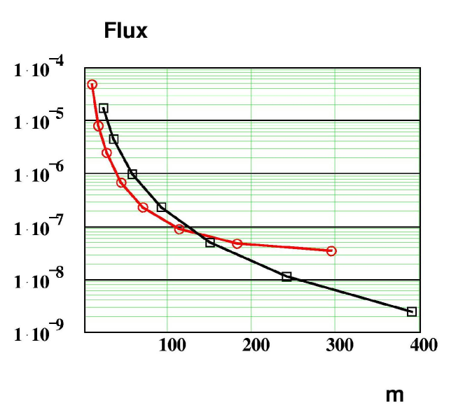
Figure 24: Comparison of the decrease of the flux across convergent island chains towards the upper Cantorus $q=N(1,7)$ (circles) and towards the KAM surface on the plasma edge $q=N(4,2)$ (squares). The former is seen to converge to a finite value of the order of $10^{-8}$, while the latter is observed with lower values to continue to decrease hopefully to zero (robust barrier).

The results can be summarized as follows. For the KAM barrier, the positive and the negative residues converges slowly to $0$, so the subcritical case in the Greene’s conjecture is verified . The possible explanation for this slow convergence is that the value of the stochasticity parameter $K=4.875$ is very near the threshold for large scale dispersion due to the breaking up the edge barrier. By computing the periodic orbit with an error of $10^{-13}$, we obtain still decreasing values of the flux of the order of $10^{-9}$, actually smaller than the flux across the Cantorus. So, we may expect the convergence towards $0$.

For the Cantorus, the values of the flux are actually comparable with the values for the KAM for small periods, but the last we were able to compute is of the order of $10^{-9}$. The Fig.(24) shows that it seems to already converge towards a value larger than the one obtained for the KAM.

In conclusion, the Greene’s conjecture and Mather’s theorem are verified in both situations and the numerical results are in agreement with the theory. From Fig.(24) we can thus conclude that the existence of (i) a KAM surface, the plasma edge barrier,  having the rotation number $\frac{1}{N\left(4,2\right)}$ and of (ii) a partial barrier, a Cantorus, with the rotation number $\frac{1}{N\left(1,7\right)}$ was indeed confirmed by using numerical methods.

6 Asymptotic radial subdiffusion

Dispersive motion of magnetic lines in a stochastic zone is often described very roughly as a random walk. We stress the fact that the radial motion observed here is non-diffusive. In order to determine more precisely the average dispersion properties of magnetic lines in a situation of incomplete chaos (diffusion, subdiffusion or superdiffusion) and their scaling properties with the perturbation, we have calculated the asymptotic properties of a set of $5000$ magnetic lines. Initial conditions are chosen in the chaotic shell on an initial circle $\psi=0.001$, $r\sim 0.0316$, outside of the protected plasma core, either as a bunch of lines within a small angular interval $\Delta\theta=0.001$, or on a complete circle with regularly spaced initial values of the initial angle $\theta$ between $0$ and $1$. The values of the stochasticity parameter $L$ are varied in a wide range between $0.776$ and $6.68$, beyond the threshold for large scale chaos above which all magnetic lines from the chaotic shell finally cross the edge barrier, transformed into a permeable Cantorus. Here we also study the radial position $x=\sqrt{\psi}$ of a magnetic line, which is unity on the unperturbed plasma edge.

We have to stress the fact that with such large values of the stochasticity parameter $L$, almost all magnetic lines in the central chaotic shell are crossing the plasma edge. This situation is of course of less interest for confinement studies. It would rather be characteristic, instead, of a situation of plasma disruption due to the rapid escape of the magnetic lines. The time behavior of this escape is however interesting in order to study the scaling properties of this dispersive motion, as compared with other maps like the standard map, where a similar flux diffusion has been intensely studied since many years.

6.1 Long time behavior

Although the individual motion of one magnetic line appears to be discrete and random, average properties like the mean poloidal flux $\psi_{m}$ and the mean radius, averaged over initial conditions, can be described by ”continuous” functions of ”time” (the number of large turns around the torus) :

$$\psi_{m}(t)\equiv\left\langle\psi(t)\right\rangle\text{ \ \ \ \ , \ \ \ \ \ \ }x_{m}(t)\equiv\left\langle\sqrt{\psi(t)}\right\rangle\text{, \ \ \ \ \ \ \ }$$ (94)

In order to deduce dispersion properties, we also calculate a third independent quantity : the mean square displacements (MSD) of the flux, defined in the reference frame of the average motion :

$$MSD_{\psi}(t)\equiv\left\langle\left[\psi(t)-\psi_{m}(t)\right]^{2}\right\rangle$$ (95)

The MSD of the radius is also computed, and we check that the following exact relation is verified at each time in terms of the average motion :

$$MSD_{x}(t)\equiv\left\langle\left[\sqrt{\psi(t)}-x_{m}(t)\right]^{2}\right\rangle=\psi_{m}(t)-x_{m}(t)^{2}$$ (96)

The intuitive picture emerging from these results is the dispersion of magnetic lines from an initial circle of intersection points, passing local weak barriers, coming back an forth and expanding radially in average. The asymptotic state of course strongly depends on the value of the stochasticity parameter $L$ , as well as all characteristic times which appear to scale like $L^{-2}$ (see Eqs.(102) below).

6.1.1 Asymptotic motion in the confined domain

In the confinement domain, the global diffusion of course vanishes, but the details of the time behavior of an ensemble of magnetic lines is characteristic of the phase portrait presented in Fig.(11). For $L=4.875/2\pi\sim 0.776$, the orders of magnitude of the characteristic times can be inferred from Fig.(13) and tested in the present average evolution : residence times inside the ITB would be of the order of $\tau_{ITB}\approx 10^{6}$ (downwards peaks), residence times in the chaotic shell would be of the order of $\tau_{shell}\approx 10^{7}$ and in the chaotic sea of the order of $\tau_{sea}\approx 10^{8}$ iterations.

$$\vskip 12.0pt plus 4.0pt minus 4.0pt\begin{array}[]{cc}\tau_{ITB}\approx&10^{6}\\ \tau_{shell}\approx&10^{7}\\ \tau_{sea}\approx&10^{8}\end{array}$$ (97)

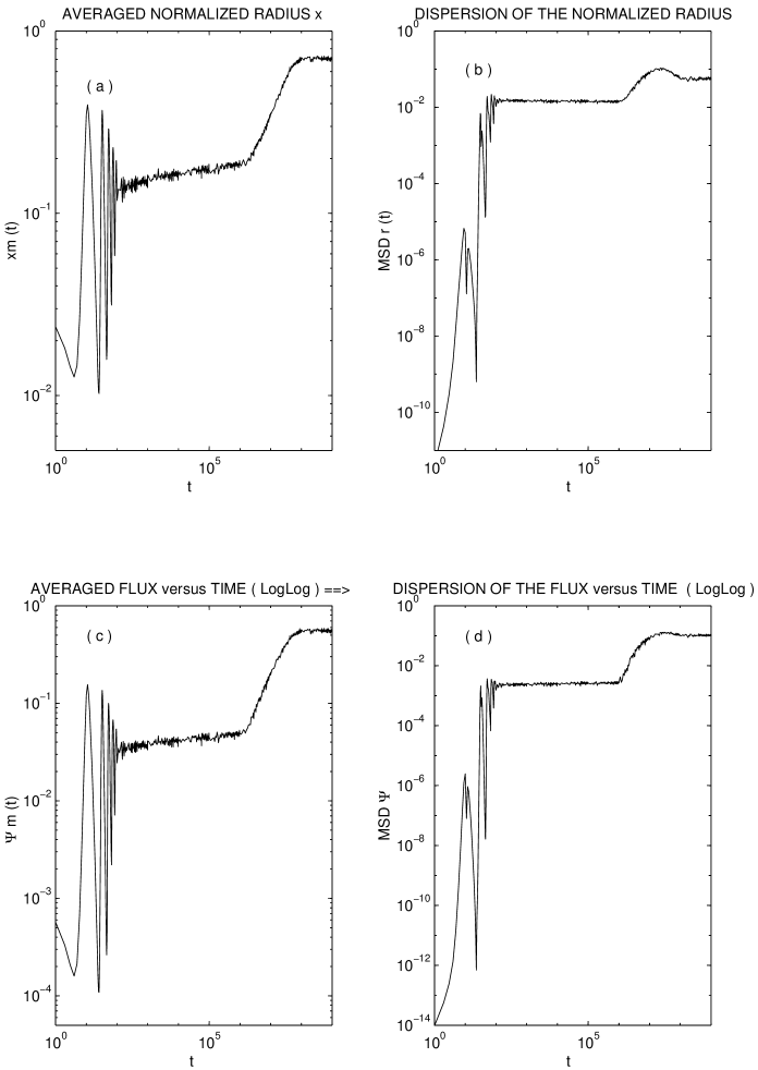
Figure 25: Average radius (a), mean square radial dispersion (b), average flux (c) and mean square flux dispersion (d) of an initial bunch of $500$ lines at $L=4.875/2\pi$ followed during $10^{9}$ iterations.

We first consider a bunch of $500$ initial conditions within $\Delta\theta=0.001$ followed over $10^{9}$ iterations for $L=4.875/2\pi\sim 0.776$. We observe that none of the $500$ considered magnetic lines succeeds to escape from the plasma edge even after $10^{9}$ iterations, and the average radius saturates around a value $x_{m}(t)$ $\sim 0.7$ which proves that the robust KAM barrier on the plasma edge is still resistant (see Figs.(13) and (11)). The detailed form of the time dependence is however interesting, especially concerning the average radius $x_{m}(t)$ and the radial dispersion $MSD_{x}(t)$ (see Fig.(25). In Fig.(25.a) which represents  $x_{m}(t)$, we see at short times large oscillations starting from the initial condition $x\sim 0.0316$ and saturating after about $10^{2}$ iterations; this can be explained by the motion of the bunch of lines as a whole, along the non circular magnetic surfaces making an excursion towards larger $x$ values at each poloidal turn in $\theta$.

For larger times, up to $10^{6}$, a slow increase of the average value is observed up to a value $x_{m}(t)$ $\sim 0.2$, while the dispersion remains constant (Fig.(25.b)). This value $x_{m}(t)$ $\sim 0.2$ is important since it roughly corresponds to the position of the transport barrier (averaged along $\theta$). The resulting interpretation is the following : the ensemble of magnetic lines describe a CTRW with long sojourn times inside (or below) the ITB, so that the average position does not exceed that of the ITB. The dispersion remains constant (zero diffusion) since the chaotic motion occurs inside a restricted region below the upper Cantorus of the barrier.

Understanding the global motion for longer times, between $10^{6}$ and $10^{8}$, appears as a challenging question. It is seen indeed in  Fig.(25.a) that the average radius suddenly begins to increase in time (roughly like $t^{1/2}$), while the dispersion $MSD_{x}(t)$ (Fig.(25.b)) first increases (roughly like $t^{1}$) from $10^{6}$ to $10^{7}$, has a maximum and then decreases toward a constant value. An interpretation of this overshooting can be tentatively proposed as follows.

- For times shorter than $\tau_{ITB}\approx 10^{6}$ the dispersion is dominated by the trapping processes inside the ITB, and the very few lines which succeed to escape across the barrier actually create a slow increase of the curve.

- Then from $\tau_{ITB}\approx 10^{6}$ to $\tau_{shell}\approx 10^{7}$ usual diffusion occurs in the chaotic shell and $MSD_{x}(t)$ grows linearly in time.

- Around $\tau_{shell}\approx 10^{7}$ saturation of the dispersion is observed because of the finite size of this chaotic shell limited by the ITB.

- After $\tau_{shell}\approx 10^{7}$ a non negligible part of the magnetic lines are in the chaotic sea, and long sticking events occur around the main rational chains (see Fig.(22)) which result in a decrease of the dispersion.

- Final saturation of the dispersion is obtained around $\tau_{sea}\approx 10^{8}$ with an average value $x_{m}(t)$ $\sim 0.7$.

This average position of the magnetic lines can also be roughly explained in terms of the estimated average residence times : each region (chaotic shell, ITB and chaotic sea) has indeed an average radial position (averaged over  $\theta$), and when these average positions are weighted by the percentage of time spent in each region, one finds indeed a result of the order of the asymptotic radius observed in Fig.(25.a): $x_{m}(t)$ $\rightarrow 0.7$. Such an agreement should not be taken too seriously, and very long iterations should be necessary in order to compute accurate residence times for this presumed CTRW, but the orders of magnitude found yield a first explanation.

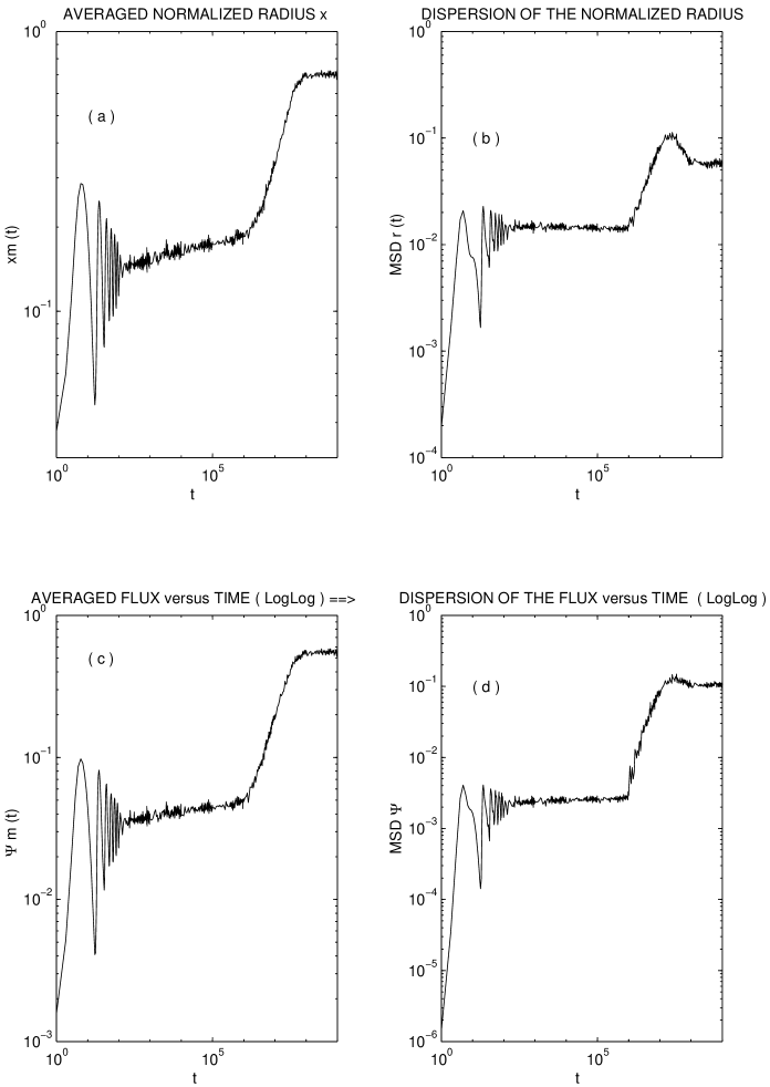
Figure 26: Average radius (a), mean square radial dispersion (b), average flux (c) and mean square flux dispersion (d) of an initial circle of $5000$ lines at $L=4.875/2\pi$ .

When the same calculation is performed for an initial circle of magnetic lines starting from the same value $\psi=0.001$, $r\sim 0.0316,$ analogous results are obtained in Fig.(26) except for the short time oscillations which are of smaller amplitude but which however remain.

6.1.2 Asymptotic motion in the transition domain

For a slightly higher value of the stochasticity parameter $L=5/2\pi\sim 0.796$, the same series of transitions occurs at small value of the ”time” : we may thus consider shorter asymptotic times and a larger number of initial conditions. For such $L$ value, all magnetic lines actually go beyond the plasma edge, indicating that the KAM on the edge is already broken, transformed in some Cantorus. The latter still represents some barrier, and the average motion is different inside and outside this permeable barrier.

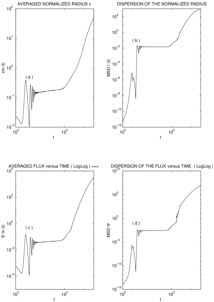
Figure 27: Average radius (a), mean square radial dispersion (b), average flux (c) and mean square flux dispersion (d) of an initial circle of $5000$ lines at $L=5/2\pi$.

In Figs.(27.a to d) we have represented the four functions $x_{m}(t)$, $MSD_{x}(t)$, $\psi_{m}(t)$ and $MSD_{\psi}(t)$ for a bunch of $5000$ initial lines. Clearly a similar transition region is obtained, as in Figs. (25) and (26), but here for smaller values of time (roughly from $10^{5}$ to $10^{6}$). In this time domain a straight line is observed in each graph, corresponding to the following transient time behaviors: $x_{m}(t)\sim t^{1/2}$, $MSD_{x}(t)\sim t^{1}$, $\psi_{m}(t)\sim t^{1}$ and $MSD_{\psi}(t)\sim t^{2}$ which represent a transient diffusion of the radius and a superdiffusion of the flux $\psi$. For such an initial bunch of lines, the initial oscillations are well pronounced. Here the asymptotic behavior is not yet reached after $10^{8}$ iterations and it seems that the dispersion of the radius $MSD_{x}(t)$ could tend to a constant value, probably because of the presence of a resistant barrier very far out of the plasma. The latter is of no physical relevance for the tokamak, but is however characteristic of the present process of destruction of successive barriers in an incomplete chaos situation.

6.1.3 Asymptotic motion in the large scale dispersion domain

Beyond such transition region, for $L=5.5/2\pi\sim 0.875$ the time behavior is more regular. In Fig.(28.a to d), we have represented the four function $x_{m}(t)$, $MSD_{x}(t)$, $\psi_{m}(t)$ and $MSD_{\psi}(t)$. As expected the initial oscillations are less pronounced, but still exist. Some transient behavior can hardly be seen (around $10^{3}$ in $MSD_{\psi}(t)$) and a rapid growth leads to a final asymptotic state reached after $10^{5}-10^{6}$ iterations, in which a simple time behavior is measured.

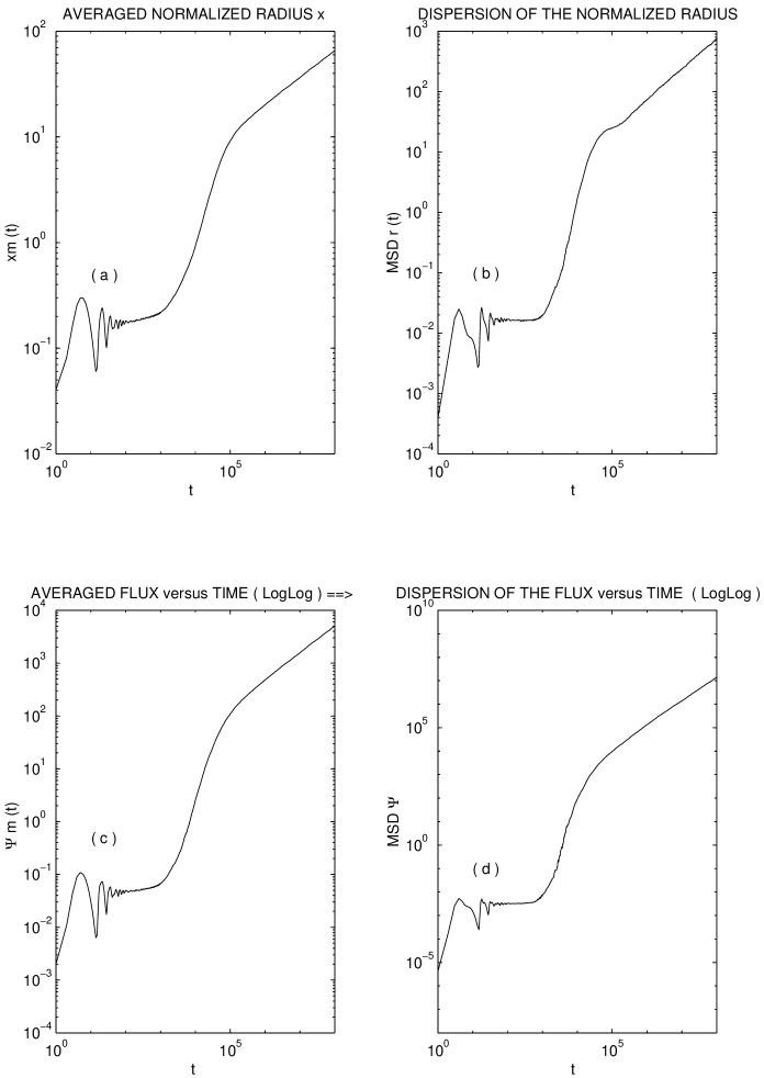
Figure 28: Average radius (a), mean square radial dispersion (b), average flux (c) and mean square flux dispersion (d) of an initial circle of $5000$ lines at $L=5.5/2\pi$.

One notes a common (but not fully understood) feature of all the graphs in that domain of $L$-values: all these functions seem to present an inflection point when reaching the absolute value unity. In the graphs for $x_{m}(t)$ this occurs at a time of physical relevance, called the escape time $t_{\varphi}$ (the time to reach the edge of the plasma at $\psi=1$, $x=1$, such that $x_{m}(t_{\varphi})=1$) which is here $t_{\varphi}\approx 10^{4}$.

In Fig.(28.b) for $MSD_{x}(t)$ we remark that some overshooting of the curve appears around $10^{5}$, before the asymptotic state is reached. Such bump does not appear on the other functions. Is it simply the effect of a distant barrier, out of the plasma edge, which temporarily traps magnetic lines ?

Such a bump also appears in Fig.(29.b) for $MSD_{x}(t)$ at a higher value $L=6/2\pi\sim 0.955$ for an initial bunch of $5000$ lines. In each of the Figs.(29.a to d), all the features remain unchanged, except that the escape time is decreased  $t_{\varphi}\approx 10^{3}$  and that asymptotic state is reached more rapidly, around $10^{4}$.

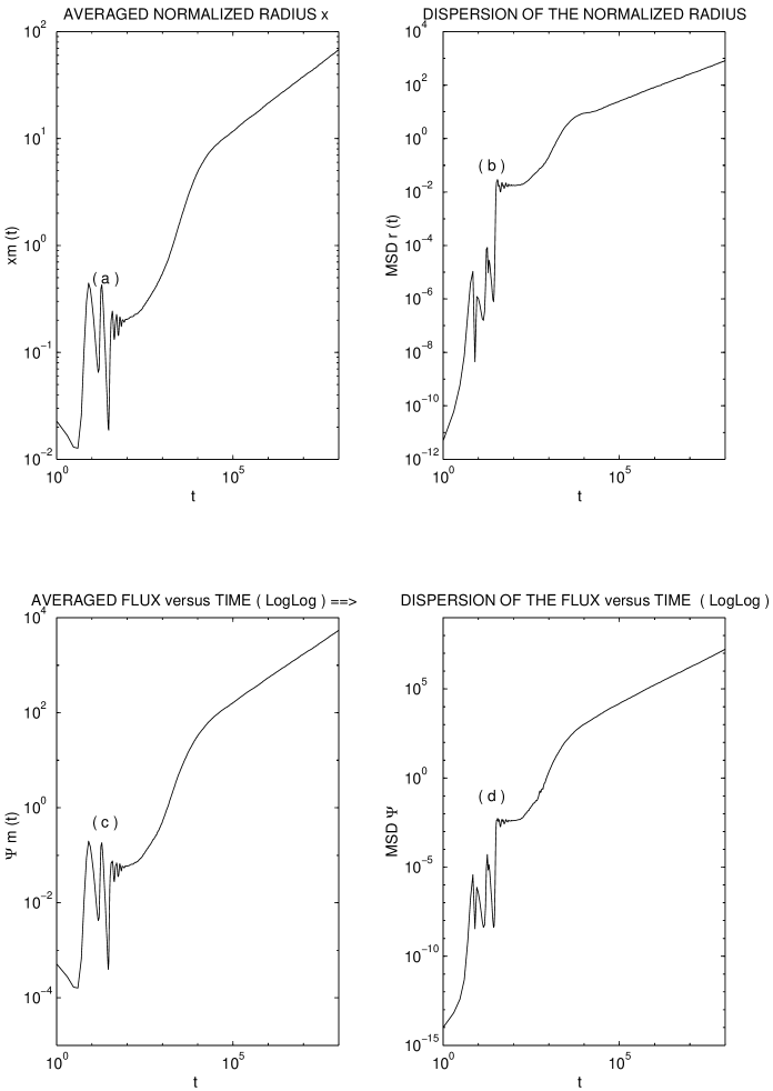
Figure 29: Average radius (a), mean square radial dispersion (b), average flux (c) and mean square flux dispersion (d) of an initial bunch of $5000$ lines at $L=6/2\pi$.

For higher $L$ values $L=9/2\pi$, dispersion is still more rapid and the asymptotic state is reached more rapidly. Here we follow a circle of $5000$ initial lines. One note however in Figs.(30.a to d) that the curve in log-log scale has a long time slope which is slowly decreasing towards what we consider as the asymptotic state, so that long iterations are necessary to evaluate accurately the time behavior and the dispersion coefficients introduced below (see Eqs. (102) ).

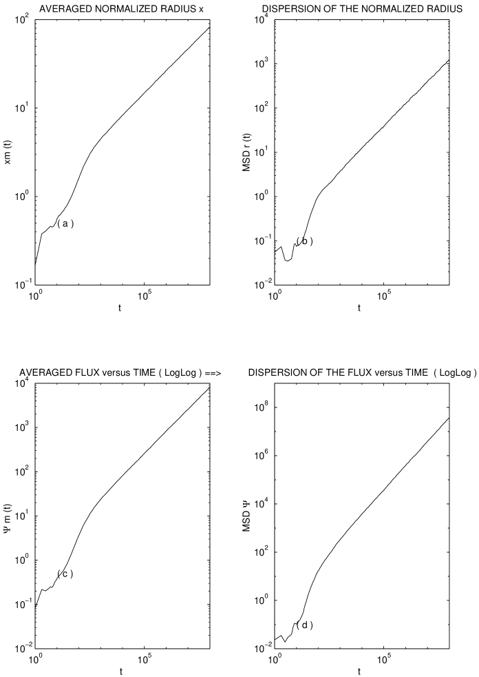
Figure 30: Average radius (a), mean square radial dispersion (b), average flux (c) and mean square flux dispersion (d) of an initial circle of $5000$ lines at $L=9/2\pi$.

For a set of values of the stochasticity parameter $L$ in the large scale dispersion domain, we have measured the asymptotic slope and dispersion coefficient of each quantity (94 to 96). Our measurements indicate that the average radius is found to increase asymptotically in time as $t^{1/4}$ :

$$x_{m}(t)\rightarrow a\text{ }t^{1/4}$$ (98)

In a consistent way we find

$$\begin{array}[]{ccc}\psi_{m}(t)\rightarrow b\text{ }t^{1/2}&\text{,}&MSD_{\psi}(t)\rightarrow 2\text{ }D_{\psi}\text{ }t\end{array}$$ (99)

i.e. diffusion of the flux, like in the standard map, and of course

$$MSD_{x}(t)\rightarrow 2\text{ }D_{x}\text{ }t^{1/2}$$ (100)

which means radial sub-diffusion. Although surprising, this is however not a fully new result: similar phenomena of  ”strange” transport ¹⁴ [60] (where $MSD_{r}(t)\sim t^{\mu}$ with $\mu\neq 1$) have been measured, namely for charged particles sticking around an island remnant in a chaotic three-wave chaotic model [61] resulting in a $t^{1/3}$ behavior [62].

It has to be noted that, with the same unperturbed magnetic field (35), the direct integration of the magnetic line equations of motion, in presence of Fourier series magnetic perturbations or a distribution of current filaments, has already yielded a fully equivalent $t^{1/4}$ asymptotic behavior the quantity $\sqrt{MSD_{x}(t)}$ rapidly called by these authors as being some ”average displacement” of magnetic lines in chaotic layers [63]. This $t^{1/4}$ law is in total agreement with the results (100) obtained here in a simple map.

The above subdiffusive result (100) is however reached asymptotically for long times. In the present incomplete chaotic regime of the tokamap, it shows a slower dispersion ($\mu<1$) which is different from the usual diffusion in a completely chaotic situation [64]. A comparison is performed below, after Eq.(112) and in Fig.(32), in Section 6.4.

For physical times, of the order of the average time $t_{\varphi}$ necessary to escape from the boundary circle, different transient regimes are observed instead, with a rapid radial super-diffusion ($\mu>1$) observed when crossing the plasma edge. In other words, although the asymptotic, long time properties are diffusion of the flux and sub-diffusion of the radius, several other behaviors are observed along the time evolution, with a slower or faster time variation.

The numerical results measured for the coefficients $a$, $b$, $D_{x}$ and $D_{\psi}$ are the following, as function of the stochasticity parameter $L:$

$$\begin{array}[]{ccccc}L&a&b&D_{x}&D_{\psi}\\ 0.836&0.625&0.460&0.035&0.060\\ 0.875&0.651&0.500&0.038&0.070\\ 0.955&0.673&0.534&0.041&0.081\\ 1.321&0.795&0.745&0.057&0.158\\ 1.671&0.899&0.952&0.072&0.255\\ 2.149&0.972&1.150&0.103&0.409\\ 2.387&1.029&1.276&0.108&0.496\\ 2.626&1.119&1.478&0.112&0.621\\ 3.342&1.209&1.789&0.163&1.005\\ 4.138&1.403&2.327&0.180&1.551\\ 4.775&1.498&2.657&0.207&2.040\\ 5.252&1.579&2.947&0.226&2.484\\ 6.048&1.691&3.393&0.267&3.373\\ 6.685&1.638&3.421&0.369&4.133\end{array}$$ (101)

6.2 Scaling properties

Another important feature of transport processes is the scaling property of the corresponding dispersion coefficients (101) in terms of the perturbation parameter $L$. In order to draw the scaling laws for these coefficients, we define arbitrarily the first values by $L_{o},a_{o},b_{o},D_{xo}$ and $D$ and we plot the above numerical results reduced to these first values as $L/L_{o},a/a_{o},b/b_{o},D_{x}/D_{xo}$ and $D_{\psi}/D_{\psi 0}$, respectively.

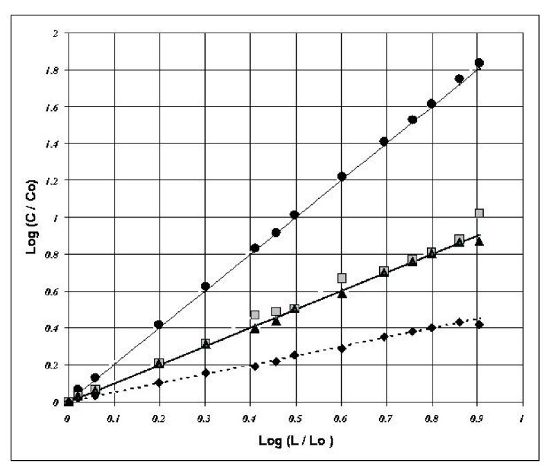
Figure 31: Graphical presentation of the scaling dependence in the stochasticity parameter $L$ of the asymptotic coefficients of flux diffusion $D_{\psi}\sim L^{2}$ (black circles), of radius subdiffusion $D_{x}\sim L$ (grey squares), of average flux growth $b\sim L$ (black triangles) and average radius growth $a\sim L^{1/2}$ (black diamonds).  For a lowest value $L_{0}=5.25/2\pi\sim 0.836$ this graph represents these various coefficients $C$ in a logarithmic plot of $\log(C/C_{0})$ as function of $\log(L/L_{0})$. The three straight lines correspond, from top to bottom, to the expected behaviors in $L^{2}$, $L$ and $L^{1/2}$, respectively.

We clearly see in Fig.(31) that the various coefficients scale as follows : $a(L)\sim L^{1/2}$, $b(L)\sim L\sim D_{x}(L)$ and $D_{\psi}(L)\sim L^{2}$.

Summarizing the results obtained for the both dependences in $L$ and $t$ (see Section (4)), we can write down the following asymptotic formulas describing both the long time dependence (Eq.(98) to (100)) and the scaling properties of the so-defined dispersion coefficients $a(L)$, $b(L)$, $D_{x}(L)$ and $D_{\psi}(L)$ :

$$\begin{array}[]{c}\lim_{t\rightarrow\infty}x_{m}(t)=a(L).t^{1/4}\simeq\left[L^{2}t\right]^{1/4}\\ \lim_{t\rightarrow\infty}\psi_{m}(t)=b(L).t^{1/2}\simeq\left[L^{2}t\right]^{1/2}\\ \lim_{t\rightarrow\infty}MSD_{x}(t)=2\text{ }D_{x}(L).t^{1/2}\simeq\left[L^{2}t\right]^{1/2}\\ \lim_{t\rightarrow\infty}MSD_{\psi}(t)=2\text{ }D_{\psi}(L).t\simeq\left[L^{2}t\right]\end{array}$$ (102)

This clearly shows a global scaling in $\left[L^{2}t\right]$ . Such scaling laws can be simply interpreted as resulting from a simple intuitive law of the type $\delta\psi(L,t)\approx\left[\delta x^{2}\right]\simeq L$.

In the standard map, which is periodic in both variables angle and action, it is well known [65], [66] (see also p.299 in [19]) that computation of the diffusion coefficient of the action yields the result $D(L)=D_{ql}(L).S(L)$, where $S(L)$ involves a series of Bessel function $J(L)$, and where the simple coefficient

$$D_{ql}(L)=L^{2}/4$$ (103)

can be obtained from a random phase argument. This classical result for the standard map is actually modified by the presence of accelerator modes, which do not occur here. Beyond the scaling relation $D_{\psi}(L)\simeq L^{2}$ (Eq. (102)) found to be satisfied in the tokamap, it is interesting to compare the exact numerical results with Eq. (103). We find

$$D_{\psi}(L)\simeq D_{ql}(L).\left[1\pm 0.1\right]$$ (104)

which shows not only that the same quasi-linear diffusion coefficient $D_{ql}(L)$ applies both in the standard map and in the tokamap, but moreover that no Bessel functions seem to appear here, probably due to the lack of periodicity of the map in the flux variable.

Some methods for the calculation of diffusion coefficients in maps where variables are clearly separated are given in [67]. An analytical derivation of even a simple result like Eq.(104) for the tokamap (Eqs. (31), (32) where variables are not separated) seems however to be difficult to prove in general using the usual Fourier path diagram method [66]. It is however very simple to check that the same random phase argument can be applied to the tokamap and the same result (103) is obtained, as for the standard map but without any Bessel functions here. Unlike the standard map, this asymptotic behavior (104) is valid for all values of the stochasticity parameter $L$.

6.3 Asymptotic times and transient regime inside the plasma beyond escape threshold.

The asymptotic state for $L=5.5/2\pi\sim 0.796$ (beyond escape threshold) has been obtained after a rather long relaxation times

$$t_{R}\approx 10^{6}.$$ (105)

We have no theoretical explanation for such slow phenomenon in the tokamap, but in similar, simpler systems, relaxation times are also very long. For the standard map [28] [43], very long iteration sequences have been necessary to perform measurements of the transition probability between different basins and to characterize the corresponding CTRW. A detailed kinetic theory has been elaborated very recently [68] for the standard map, showing also very long relaxation times.

Since asymptotic behavior is only reached after such long relaxation times, of course magnetic lines are already far beyond the physical domain of the plasma ($\psi\leqslant 1$). For instance in Fig.(28.a), for a value $L=5.5/2\pi$ just after breaking of the edge KAM, we can see that the average radius $r_{m}$ reaches the edge of the (unperturbed) plasma after a ”physical” or ”escape time” $t_{\varphi}$ such that $r_{m}(t_{\varphi})=1$, which yields

$$t_{\varphi}\approx 10^{4}$$ (106)

At least for values of $L\gtrsim 5/2\pi\sim 0.796$ , beyond the escape threshold, this time represents an estimate of the escape time, or more precisely, an estimation of the number of turns (the long way) around the torus after which a magnetic line has reached the plasma edge.

It is interesting to translate the number of iterations in the tokamap (thus the number of turns) into an average time for thermal particles to reach the plasma edge by following the magnetic lines (in absence of collisional or magnetic drift effects). One iteration time step in the tokamap represents actually the length of one large turn of length $2\pi R_{0}$ around the torus. For a thermal particle following the field line the physical time (106) can thus be evaluated as the time necessary for a particle to travel $t_{\varphi}$ times the long way along the torus, i.e. $2\pi R_{0}\ast t_{\varphi}/V_{th}$. In Tore Supra, this time is of the order of $10^{-2}$ $s.$ for ions and $10^{-4}$ $s.$ for electrons in usual conditions ($T=5$ $keV$)

$$\begin{array}[]{lll}t_{\varphi\text{ }i}=10^{-2}s.&\text{,}&t_{\varphi\text{ }e}=10^{-4}s.\end{array}$$ (107)

In the same way one can deduce that the relaxation time, corresponding to $10^{6}$ iterations steps of the tokamap, actually represents $20$ $s$ for ions and $0.5$ $s.$ for electrons in Tore Supra.

$$\begin{array}[]{lll}t_{R\text{ }i}=20\text{ }s.&\text{,}&t_{R\text{ }e}=0.5\text{ }s.\end{array}$$

These are the times necessary to reach the slow asymptotic subdiffusion regime at $L=5.5/2\pi\sim 0.796$ . The transient superdiffusive regime occurring for $t<t_{R}$ is thus not excluded from the domain of practical interest, as well as asymptotic subdiffusion regime obtained here.

These values of the escape time in the tokamap (107) are thus much shorter than the particle confinement time $\tau_{P}\succeq\tau_{E}\sim 0.20$ $s.$ which is admitted to be roughly equal to the energy confinement time $\tau_{E}$, in the absence of additional heating for Tore Supra for instance. Such escape times (106) are thus relevant for particle confinement losses in tokamaks.

For times of the order of the escape time $t\lessapprox t_{\varphi}$, the average radius is growing like $x_{m}(t_{\varphi})\sim t^{1.}$, much faster than in the asymptotic state (98). The general shape of the curve Fig.(28.a) indeed indicates a slow initial growth, followed by a rapid increase of the slope, similar to an exponential growth, and a final saturation with a lower asymptotic slope. We note that the pseudo-exponential growth occurs precisely around the physical time (106).

In other words, although the asymptotic behavior of magnetic line motion in the tokamap is a rather regular one (even if a ”strange” one) described by (102), nevertheless for finite times of the order of the physical time we observe the following extremely rapid transient time-behavior :

$$\begin{array}[]{l}MSD_{\psi}(t_{\varphi})\sim t^{5.88}\\ MSD_{x}(t_{\varphi})\sim t^{2.75}\\ x_{m}(t_{\varphi})\sim t^{1.}\end{array}$$ (108)

In the transient regime occurring inside the plasma, for $L=5.5/2\pi$, we have thus a superdiffusion $MSD_{x}(t_{\varphi})\sim t^{2.75}$ of the magnetic lines, around an average radius growing like $x_{m}(t_{\varphi})\sim t^{1.}$ i.e. in a ballistic way. This last observation would seem a priori much less favorable for plasma confinement in perturbed magnetic structures, but it is actually not the case.

6.4 Comparison with classical diffusive predictions

We have to compare the present result (108) with the classical analytical prediction, i.e. the diffusion coefficient of magnetic lines in a completely stochastic magnetic field. This process is parametrized by the amplitude of the magnetic perturbation $\beta=\mid\delta B\mid/B$ and by parallel and perpendicular coherence lengths of the perturbation, $\lambda_{\shortparallel}$ and $\lambda_{\perp}$, respectively. This naturally introduces the control parameter of the problem : the Kubo number

$$\alpha\equiv\beta\frac{\lambda_{\shortparallel}}{\lambda_{\perp}}$$ (109)

which roughly measures the parallel coherence of the fluctuating magnetic field : magnetic diffusion will be small if $\alpha$ is small. The quasilinear approximation $D_{QL}$ for the diffusion coefficient in a completely chaotic field is simply :

$$D_{QL}=\frac{\lambda_{\shortparallel}}{\lambda_{\perp}^{2}}.\sqrt{\frac{\pi}{2}}.\alpha^{2}=\sqrt{\frac{\pi}{2}}\beta^{2}\lambda_{\shortparallel}$$ (110)

It is actually a quadratic approximation in the Kubo number $\alpha$ , where the first factor takes the dimensionality into account (the units of the magnetic diffusion coefficients are in $m^{2}/m$.). Higher order terms have been derived from a more general description of diffusion in a completely stochastic fields in [64]. This coefficient (110) has been originally derived in [69], [70]. The radial mean square displacement $<x^{2}(z)>=2D_{QL}.z$ is growing linearly with the toroidal distance $z$ .

In order to make a connection with physical parameters of the tokamak, we have to know the relation between the stochasticity parameter $L$ and $\beta$ the relative strength of the perturbation introduced for instance in the non-axisymmetric external coils. From the alternative derivation of the tokamap from canonical variables [32], this relation can be derived as :

$$L=\frac{2\pi}{\varepsilon_{T}}\left(\frac{\delta B}{B}\right)$$ (111)

where $R_{0}/a=1/\varepsilon_{T}$ is the aspect ratio of the torus. 

Within the present dimensionless units (reduced to the minor radius $a$ of the plasma column), and with $t$ being as previously the number of long turns around the torus, this classical result writes (with $z=2\pi R_{0}.t$, $\lambda_{\shortparallel}\approx 2\pi R_{0}$, $r^{2}=2x^{2}$ and $L=2\pi\beta/\varepsilon_{t}):$

$$MSD_{QL}(t)=\sqrt{2\pi}L^{2}t$$ (112)

It can easily be shown that this linear function (112) remains for all times much above the numerical result of Fig.(28.b), even for physical times of the order of $t_{\varphi}$ where the growth rate is like $t^{2.75}$: in Fig.(32) we draw the dispersion measurements of the radial position in the present situation of incomplete chaos for $L=5.5/2\pi\sim 0.876$ (as in Fig.(28.b)) along with its asymptotic slope (dotted line) which exhibits an asymptotic radial subdiffusion. In the domain between $t=10^{3}$ and $10^{4}$ (around the escape time $t_{\varphi}$ , see Eq. (106)), one clearly observe a superdiffusive regime. All these measured behaviors of $MSD_{x}(t)$ nevertheless appear at all relevant times to remain much smaller than the quasi-linear diffusion in complete chaos as represented by the upper straight line described by the classical Eq. (112) [69].

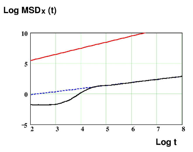
Figure 32: Dispersion measurements of the radial position in the present situation of incomplete chaos are represented (lower black curve) for $L=5.5/2\pi\sim 0.876$ (as in Fig.Dif 3b) with its asymptotic slope (dotted line) which exhibits an asymptotic radial subdiffusion. In the domain between $t=10^{3}$ and $10^{4}$ (around the escape time $t_{\varphi}$ , see Eq. 99), one clearly observe a superdiffusive regime. All these measured behaviors of $MSD_{x}(t)$ nevertheless appear at all relevant times to remain much smaller than the quasi-linear diffusion in complete chaos as represented by the upper straight line described by the classical eq. 105 of Ref.[69] (Rechester & Rosenbluth 1978).

In conclusion, the transient superdiffusion observed in the tokamap model for times of the order of the physical or escape time is actually less effective than the classical quasilinear prediction. This means that classical transport in a completely stochastic magnetic field as studied in [69], [70] and [64] is actually more dramatic for plasma confinement than the strange transport observed in the present model for incomplete chaos. A transient, very rapid growth, although ”superdiffusive” is not always ”more dangerous” than a linear one…

7 CONCLUSIONS:

The chaotic motion of magnetic lines in a toroidal perturbed geometry has been analyzed using a Hamiltonian map called tokamap [16] defined by (32, 33, 34) in terms of the stochasticity parameter $L$. It describes the successive intersection points of a magnetic line in a poloidal plane $(\psi,\theta)$ . From the previous analysis of fixed points bifurcations, new results have been derived for the Shafranov shift in this map (Fig.(1)). We restrict ourselves to the case of an monotonous unperturbed safety factor profile with a central value $q(0)=1$.

The generic phase portrait in the poloidal plane $(\psi,\theta)$ consists in a protected non-chaotic plasma core, surrounded by a chaotic shell limited by a semi-permeable Cantorus which has been identified. For increasing values of $L$ magnetic lines finally cross this first barrier and wander in a wide chaotic sea, extending up to the plasma edge (Fig.(11)). This domain of the phase portrait has the realistic structure with remnants of island chains on the dominant rational $q$-values (Fig.(4)), and sticking process of magnetic lines around these island remnants.

The important point we want to stress is that the different barriers found in this configuration always correspond to irrational values of the safety factor, and not to rational values where island chains are formed. The golden number $G$ is known to play no role in this map [37]. It is thus quite natural from KAM theory that the ”next most irrational” numbers, the ”noble” numbers $N(1,k)=1+1/(k+G^{-1})$ [17] could actually play an important role. The wandering motion in the inner shell is indeed limited by a KAM surface (or a robust Cantorus) which is located in the case $L=4.875/2\pi\sim 0.776$ downward at $q=N(1,11)=1.086..$, and upward by a semi-permeable Cantorus at $q=N(1,8)=1.116...$. The wandering motion in chaotic sea is limited downward by another identified Cantorus, which is located slightly above the previous one at $q=N(1,7)=1.131$ : we thus find the existence of a double-sided internal transport barrier. Although this barrier includes a rational surface ($q=9/8=1.125$ in the case $L=4.875/2\pi\sim 0.776$) we have shown that the two Cantori, which are actually the two sides of the barrier, are located on noble values of the safety factor. The outer edge of the chaotic sea remains a strong external transport barrier (a KAM surface or a robust Cantorus) at $L=4.875/2\pi$ ; its radial position in the $q$ -profile appears to be located with a rather good precision at the most irrational number between $q=4$ and $q=4.5$, i.e. at $q=N(4,2)=3+N(1,2)=4+1/(2+G^{-1})=4.382...$ The transport barriers observed in this map have been proved (from flux argument) to be noble Cantori. The flux of lines across permeable Cantori has been discussed in Section 5, by using very precise calculations of high order periodic points along rational chains convergent toward the Cantorus. The method used for determining these periodic point is summarized in Appendix B.

The motion along a very long trajectory shows moreover that the magnetic line motion is intermittent ( Fig.(13)), with long stages in the inner shell and in the outer chaotic sea, with occasional sticking periods around island remnants (Fig.(12)). These features are characteristic of a continuous time random walk (CTRW). The external barrier actually confines magnetic lines inside the plasma up to the appearance of a large scale motion above a threshold of the stochasticity parameter around $L\sim 5/2\pi$.

In order to describe the motion of magnetic lines beyond this large scale motion threshold, we have considered a bunch of magnetic lines in a small area of phase space and study their statistical average evolution. We have computed, the average radial position (94) of the bunch of lines, and the mean square deviation of the radius (96) compared to this average radius : this is the quantity defining the spatial diffusion properties in the asymptotic stage (subdiffusion or superdiffusion). We have also calculated the diffusion (95) of the poloidal flux $\psi$ : the latter appears to describe asymptotically a classical diffusion (in $\psi$ !) and behaves as traditionally admitted, i.e. like the standard map in the quasi-linear stage, with a diffusion coefficient in action space which scales like $D\sim L^{2}$ in the domain $L=\left[5/2\pi,21/2\pi\right]$. This diffusive behavior does not hold for magnetic lines in physical space.

Since the action of poloidal flux $\psi$ is proportional to the square of the radius $x$, this diffusion process in action is equivalent to a fourth moment of $r$. It is thus not surprising at all that the radial $r$-motion appears to be asymptotically a spatial subdiffusion

$$\begin{array}[]{llll}<\left[x(t)-x_{m}(t)\right]^{2}>\Longrightarrow 2D_{x}(L)\text{ }t^{1/2}&&\text{with}&D_{x}(L)\sim L\end{array}$$ (113)

In contradistinction with usual results for dispersion in completely chaotic situations (quasi-linear description) , the radial motion of stochastic magnetic lines in the present tokamap model, with incomplete chaos, thus appears as a radial ”strange diffusion” and not classical diffusion. In (113) $x_{m}(t)$ is the average radius

$$\begin{array}[]{llll}x_{m}(t)=<\sqrt{\psi(t)}>\Longrightarrow a(L)\text{ }t^{1/4}&&\text{with}&a(L)\sim L^{1/2}\end{array}$$ (114)

which grows asymptotically as $(L^{2}t)^{1/4}$. The scaling laws (102) for the coefficients of these three average processes reveal a nice scaling in $(L^{2}t)$ for the asymptotic diffusion properties of the tokamap, even for strange diffusion.

These general and asymptotic properties of magnetic line motion in a perturbed toroidal geometry have been obtained in the tokamap model. However, the threshold value of the stochasticity parameter $L\sim 1$ , for which particles begin to escape from the plasma to describe large scale motion and a true diffusion in action space, is sufficiently high, and the relaxation time $t_{R}$ (105), necessary to reach the asymptotic stage, is sufficiently long for this asymptotic stage to be reached when the average radial position of the bunch of lines has already crossed the plasma edge $\psi=1$. As a consequence, the magnetic line motion inside the plasma is either confined by a KAM external barrier, and the asymptotic motion can only be subdiffusive when $L<1$ (like in Ref. [43]), or escaping from the plasma when $L>1$, but this occurs in average at a physical time $t\varphi$ (106) much shorter than the relaxation time $t_{R}$, so that the motion inside the plasma is not yet the asymptotic one (see Eq. 108), and actually describes a transient regime of radial superdiffusion. This last observation could seem much less favorable for plasma confinement in perturbed magnetic structures with incomplete chaos when $L>1$, but actually the resulting motion appears to be much less dramatic for plasma confinement than the usual classical expectation from the quasilinear description of classical diffusion in completely stochastic magnetic fields [69], [70], [64].

Acknowledgements: We want to thank R. MacKay, Y. Elskens and E. Petrisor for many fruitful discussions about mathematical aspects. Four of the authors (D.C., G.S., M.V. and F.S.) have benefitted from grants from the french Ministère des Affaires Etrangères through C.E.A. Partial support is acknowledged from NATO, Linkage Grants PST.CLG.971784 and 977397.

8 APPENDIX A: Standard safety factor profile.

Standard radial profiles can be derived, within a circular cross section, by taking into account elementary observations in cylindrical geometry $(\rho,\theta,z)$. The basic assumption of the model consists in assuming a parabolic density profile with vanishing condition on the edge:

$$n(x)=n(0)\left[1-x^{2}\right]$$ (115)

where the radius $x=\rho/a$ is reduced to the small radius $a$ of the plasma. Such a profile is not inconsistent with early observations of ohmically heated plasmas [71].

Next, a general relation is assumed between temperature and density profiles. A systematic fitting of many profiles on various early tokamaks [72] indicates that the temperature profile can adequately be represented by squaring the density profile. Such a result can also be obtained from simple analytical models of energy balance (see e.g. p. 41 in  [73]). We thus consider :

$$T(r)=T(0)\left[1-x^{2}\right]^{2}$$ (116)

which also implies $\eta_{e}\equiv d\ln T_{e}/d\ln n_{e}=2.$

In order to obtain the density current profile, we assume a Spitzer dependence of the resistivity $\eta\sim T^{3/2}$ as function of the temperature [74] . For a stationary magnetic field, Faraday’s law implies indeed an irrotational electric field $\frac{\partial\mathbf{B}}{\partial t}=-\mathbf{\nabla}\times\mathbf{E}=0$ hence in an axisymmetrical system $\frac{\partial E_{z}}{\partial\rho}=0$, i.e. a constant electric field along the radius. From a simple expression of the Ohm’s law we thus find that $E_{z}(\rho)=\eta(\rho)j_{z}(\rho)=cst.$ is actually a constant along the radius $\rho$. From the temperature dependence of the Spitzer resistivity one thus deduces in this simple model that the electric current density profile is

$$j_{z}(x)=j_{z}(0)\left[1-x^{2}\right]^{3}$$ (117)

where z is the toroidal direction in cylindrical geometry. We note that Eqs. (115, 116 and 117) imply

$$\frac{\left\langle j_{z}\right\rangle_{\psi}}{j_{z}(0)}=\frac{\left\langle p\right\rangle_{\psi}}{p(0)}$$ (118)

where $p$ is the plasma pressure and $\left\langle...\right\rangle_{S}$ denotes the average inside a magnetic surface $\psi$. This relation (118) has been demonstrated to hold in ohmically heated discharges of the TCV tokamak, as quoted by Minardi [75] . He proved that the relation (118) follows from the stationarity of the magnetic entropy, in general conditions where the ohmic tokamak is considered as a ”dissipative open system in equilibrium which interacts externally with the ohmic transformer”.

We may then use Ampère’s law in cylindrical geometry

$$j_{z}=\left(\mathbf{\nabla}\times\mathbf{B}\right)_{z}=\frac{1}{\rho}\frac{d}{d\rho}\left(\rho B_{\theta}\right)$$ (119)

and integrate the current density profile (117) to obtain

$$B_{\theta}(x)=B_{\theta}(1)x\left(2-x^{2}\right)\left(x^{4}-2x^{2}+2\right)$$ (120)

where the value $B_{\theta}(1)$ on the edge is given by the total electric current $I$ in the plasma : $B_{\theta}(1)=aj_{z}(0)/8=I/2\pi a$.

In the standard model for the toroidal magnetic field the safety factor $q(\rho)$ is defined in terms of $B_{\theta}$ and on the central value $B_{0\text{ }}$of the toroidal magnetic field on the magnetic axis by $q(x)=\varepsilon_{T}xB_{0}/B_{\theta}(x)$ so that we finally obtain the safety factor profile in cylindrical geometry as

$$q(x)=\frac{4q(0)}{\left(2-x^{2}\right)\left(x^{4}-2x^{2}+2\right)}$$ (121)

This standard profiles indicates a value on the edge four times larger than on the axis $q(1)=4q(0)$ which is rather reasonable in most usual ohmic cases. By denoting $x^{2}\Rightarrow$ $\psi$, we obtain the expression actually used in [16] :

$$q(\psi)=\frac{4q(0)}{\left(2-\psi\right)\left(\psi^{2}-2\psi+2\right)}$$ (122)

where $\psi$ varies from $0$ in the center to $1$ on the edge.

In order to make use of traditional canonically conjugated coordinates $\left(r,\theta\right)$, see Eq.(36), we may also introduce $r^{2}/2=x^{2}$

$$\psi=\frac{r^{2}}{2}$$ (123)

where the modified coordinate $r\equiv x\sqrt{2}$ varies from $0$ in the center to $\sqrt{2}$ on the edge. The difference between $x=\rho/a$ and $r=\rho\sqrt{2}/a$ may simply be interpreted in terms of the $r$ as occurring in a plasma of radius $\sqrt{2\text{.}}$ In either way the edge of the plasma is located at $\psi=1$, $x=1$, $r=\sqrt{2}$ and we generally use plots in terms of the radius $x$ varying from $0$ to $1$ inside the unperturbed plasma edge.

9 APPENDIX B: Numerical method for finding periodic points in discrete maps

In this appendix we explain how to determine hyperbolic and elliptic periodic points, by a numerical algorithm derived from a generalization of the Fletcher-Reeves method, involving the Jacobi matrix of the tokamap. More details are given in [76].

The existence of points with everywhere dense trajectories and the  possibility to approximate every point by a periodic point are two important and apparently contradicting aspects of chaotic systems. Nevertheless, the localization of many periodic points appears highly necessary in order to describe the structure of the phase space. This is because a typical Hamiltonian system appears to belong to an intermediate category between completely integrable and globally chaotic systems. Their phase space decomposes in a well organized architecture of invariant subdomains. In this architecture the periodic points play the role of a skeleton. The knowledge of their relative positions and residues, permits to determine, at least qualitatively, the whole phase space structure.

The residue’s absolute value (see Eq.(76)) of hyperbolic periodic points increases exponentially with the order of periodicity $m$. This exponential increase imposes clear restrictions on the practical possibility of numerical localization of the higher order hyperbolic periodic points. The localization of periodic points approaching an invariant circle is facilitated by a - let us say a continuity principle, as follows. Consider the residue of a sequence of chain of elliptic or hyperbolic points, convergents of an irrational, generic, KAM barrier : then the residues of periodic orbits will approach the residues of the invariant circle, i. e. will  approach to zero (Greene’s conjecture [14]). In any neighborhood of an invariant circle there are elliptic  and direct hyperbolic points.

A quite inverse phenomenon occurs at half-permeable barriers, the Cantori, where the typical values of the residues tend to $-\infty$ for direct hyperbolic points and to $+\infty$ for inverse hyperbolic points.

9.1 Methods for computing periodic points (theoretical aspects)

We precise that in the following, the angular coordinate (denoted by $x_{1}$) will not be a priori reduced modulo $1$, despite the fact that in the numerical calculations, for an increased numerical accuracy, we separately represent the integer and the factional part of the angular variables. After each iteration, the integer and fractional parts of the angle are  computed and stored separately.

For our purpose, in order to find a periodic point of order of periodicity $m$ and $q=m/n$, we must solve a system of a nonlinear equation, like

$$x_{1} = TM_{1}(\ x_{1},x_{2})-n$$ (124)

$$\ x_{2} = TM_{2}(\ x_{1},x_{2})$$

where $TM=T^{m}$ is the $m$ times iterate of the original map $T$. The first equation simply expresses the fact that the $m^{th}$ iterate $TM_{1}(x_{1},x_{2})$ of the angular coordinate has the same value as the initial one ($x_{1})$ but increased by the integer number  $n$ of periodic points.

The problem of localizing periodic orbit is reduced to solving a system of nonlinear equations.

More generally, we can consider the following problem: elaborate an algorithm for solving the system of $N$ nonlinear equations

$$F_{i}(\mathbf{x})=F_{i}(x_{1},x_{2},..x_{N})=0\ \text{\ \ \ \ \ \ \ \ \ \ \ \ \ \ \ \ \ \ \ \ \ (}1\leq i\leq N\text{)}$$ (125)

by using the values of the functions $F_{1},$ $F_{2},...,$ $F_{N}$.

There are a lot of numerical methods for solving systems of nonlinear equations. Because of the large roundoff errors we are obliged to choose a very rapidly convergent method. We chose the Fletcher-Reeves minimizing method because it has a very rapid convergence (double exponential) and a basin of attraction which is large enough.

Well known iterative methods seem to be not appropriate for our aim. Consider for instance the traditional Newton iterative method [77]. It is known to converge quadratically (near the exact root, the number of significant digits approximately doubles at each step) if the initial point is chosen in the basin of attraction of the root, but the global convergence properties are very poor and unpredictable [77]. The basin of attraction is usually a fat fractal set whose boundary can be very near the root, so that the choosing the initial point is a real problem.

In our explicit computations, for higher periodic points (of periodicity $m>100$), the domain of attraction (convergence) reduces so much that it appears very difficult to localize it (as difficult as to find the periodic point itself).

There also exist numerical methods which converge exponentially but which have a much larger basin of attraction than the Newton method: minimizing methods for instance.

9.1.1 Minimizing methods

The initial problem, that of solving the system (125), is equivalent to minimizing the function $f$ defined by

$$\ f(\mathbf{x})=\sum_{j=1}^{N}(F_{j}(\mathbf{x}))^{2}.w_{j}$$ (126)

The weights $w_{j}$  are positive and are chosen according to dimensionality and relative precision criteria. In our case we simply choose $w_{i}=1$ .

Like in the case of solving nonlinear, non-algebraic equations, there exist only iterative minimization methods, which find the relative minimum closest to the starting point. The determination of an appropriate starting point will be a separate problem.

The most efficient minimization methods make use as much as possible of the differentiability properties of the functions to be minimized (called the ”objective function”).

We will consider only this class of methods. In all of this class of methods, the important step is considered to be the choice of a direction, along which the one-dimensional minimization is performed, starting from a previous approximation. How to make the most efficient one directional minimization, is usually not treated in the literature. In contrast, we will treat these two problem together.

Let $\mathbf{d}=(d_{1},...,d_{N})$ be a direction, and let $\mathbf{a}=(a_{1},...,a_{N})$ be some approximation of the minimum point, to be improved. Let us consider the following function of a single variable $t$:

$$G(t)=f(\mathbf{a+d}.t)$$ (127)

where$\ f$ is given by (126) and

$$\mathbf{x=a+d}.t$$ (128)

The derivative at $t=0$ is:

$$G^{\prime}(t=0)=\sum_{j=1}^{N}d_{j}.\left[\frac{\partial f(\mathbf{x})}{\partial x_{j}}\right]_{\mathbf{x}=\mathbf{a}}=\langle\mathbf{d,(\mathbf{\nabla}f)}_{\mathbf{x}=\mathbf{a}}\rangle$$ (129)

9.1.2 The Laplace method

The oldest method is the Laplace, or the so-called steepest descent method.  The Laplace method consists in the following choice

$$\mathbf{d=-(\nabla}f)_{\mathbf{x}=\mathbf{a}}$$ (130)

such that $G^{\prime}(t=0)<0$ and that $G$ decreases along positive values of $t$, at least at the beginning. A Laplace iteration consists in finding the minimum $t_{1}$ along this direction, in moving to this new point $\mathbf{a}_{1}\mathbf{=a+d.}t_{1}$, in computing a new direction $\mathbf{d}_{1}\mathbf{=-(\nabla}f)_{\mathbf{x}=\mathbf{a}_{1}}$ by (130) in the new point and in repeating this procedure up to desired precision is reached.

Clearly this method cannot be the best one because it is not invariant with respect to the coordinate changes, even for linear transforms: from (127) $\mathbf{d}$ must be a contravariant vector, while from (130) it is a covariant one. This lack of invariance appears more clearly in the case where the $x_{i}$ variable components are physical quantities of different kind, so that this Laplace method cannot be optimal. Nevertheless, the method works exactly, if $f(\mathbf{x})$  is of the form

$$f(\mathbf{x})=g_{1}(x_{1})+..+g_{N}(x_{N})$$ (131)

where the $g_{i}$ are functions of a single variable.

Another drawback of the Laplace method is related with the fact that even in the case where $f(\mathbf{x})$ is a polynomial of second order, it remains approximative, i.e. it requires an infinite number of iterations to reach the exact result; excepted in the case where it is of the form (131). Even worse, the rate of convergence is of the order $O((\Lambda-\lambda)/(\Lambda+\lambda))$  where $\Lambda$  and $\lambda$  are the largest and smallest eigenvalues of the associated quadratic form  (they are nonnegative, otherwise the minimum would be $-\infty$ ). If  $\Lambda\gg\lambda$ the convergence rate is very slow.

The above mentioned problems can be solved by another class of methods, known as ”conjugated direction method” ( the etymology will be explained below).

9.1.3 Conjugated direction method

The methods in this class have the following properties:

A) If $f(\mathbf{x})$ is a second order polynomial, then the method is exact in N steps  .

B) For computing the directions of successive one-dimensional minimizations, at most the first order derivatives are used.

An important consequence of property A) is the very quick rate of convergence, in the general, nondegenerate case: the error decreases like

$$O(\exp(-k.2^{p}))\$$ (132)

where $k$ is a positive constant depending on initial guess and $p.N$ is the total number of iterations.

This  conjugated direction method consists in :

(i) approximating locally, at each iteration step, the objective function by a second order polynomial

(ii) finding a linear change of variables so that this polynomial becomes of the form of (131).

The step (ii) is equivalent to finding a new coordinate system, generated by the conjugated directions $\mathbf{d}_{1}\mathbf{,d}_{2}\mathbf{,...,d}_{N}$ obtained by the $N$ successive minimizations, such that

$$\langle\mathbf{d}_{i}\text{ },\mathbf{Q.d}_{j}\rangle=0\ \ \text{if \ \ }i\neq j\ \ \$$ (133)

where $\mathbf{Q}$ is the Hessian matrix, i.e. is the matrix of the second order derivatives of the objective function. The relation (133) can be reinterpreted in the following way. The Taylor approximation of the objective function to be minimized can be written as

$$f(\mathbf{x}_{0}\mathbf{+h})=f(\mathbf{x}_{0})+\langle\mathbf{b}\text{ }\mathbf{,h\rangle+\langle h}\text{ }\mathbf{,Q.h\rangle/}2\ +O(|h|^{3})\ \ \ \$$ (134)

where $\mathbf{b=}\nabla f(\mathbf{x}_{0})=\mathbf{(\nabla}f\mathbf{)}_{\mathbf{x}_{0}}$ and $\mathbf{Q=}\left\|\frac{\partial^{2}f}{\partial x_{i}\partial x_{j}}\right\|_{\mathbf{x}_{0}}$. In Eq.(134) the quadratic term $\mathbf{\langle h}$ $\mathbf{,Q.h\rangle}$ defines a new scalar product denoted by square brackets:

$$\ \left[\mathbf{x,y}\right]=\langle\mathbf{x}\text{ }\mathbf{,Q.y\rangle}$$ (135)

The relation (133) expresses the orthogonality $\left[\mathbf{d}_{i}\mathbf{,d}_{j}\right]$ $=0$ of the conjugated directions obtained at the $i-th$ and $j-th$ minimization, relative to this new scalar product. Geometrically this means that in the new coordinate system, defined by the conjugated directions (see below how to generate these ones), the level surfaces (let us say in $3$ dimensions) are homothetic ellipsoids, with the same center, proportional semi-axis, and axes along coordinate axes. The conjugated directions are the coordinate axes. Clearly, the minimum (the center) is reached by a succession of $3$ steps, minimizing along coordinates.

From the above explanation it follows that the  $2^{d}$ order Taylor expansion term in Eq. (134) of the objective function generates (locally) a natural, canonical Euclidean geometry, in the space of variables which can be of very different  significance.

Remark: Unfortunately, all of these general purpose algorithms are local. They require an initial point to start in order to find some local minimum in the neighborhood ( in fact a basin of attraction or ” hydrographic basin”  to which the initial point belongs; their boundaries are regular, not fractal like the basin of convergence of the Newton iterations).

9.1.4 The Fletcher-Reeves method

There are different ways to generate the conjugated directions.  For most of applications the optimal one is the so called Fletcher-Reeves method [78]. The optimality refers to the reduced number of operations and storage requirement of order $O(N)$ to generate the conjugated directions, by a recursive process, using the gradients of the objective function.

One main iterative step (which minimizes exactly a quadratic function) consists in $N$ sub-steps. Each sub- step, indexed by $k$, denoted by $S_{k}$ consists in the following operations. Denote by $\mathbf{x}_{0}$ the point obtained in previous step or just the initial guess of the minimum point, by $\mathbf{d}_{0}$, the first conjugated direction.

Sub-step $S_{0}$ :

At the first substep ($k=0$ ) we take

$$\mathbf{d}_{0}=-\nabla f(\mathbf{x}_{0})$$ (136)

Compute the point $\mathbf{x}_{1}$ by minimizing the function $f(\mathbf{x}_{0}+t.\ \mathbf{d}_{0})=\psi_{0}(t)$ with respect to variable $t$. This is performed here by using simply the Newton method (see next Section). Let the optimal value be$\ t^{\ast}$. Then $\mathbf{x}_{1}=\mathbf{x}_{0}+t^{\ast}.\ \mathbf{d}_{0}$

Suppose we performed the sub-steps $S_{0}$ , …, $S_{k}$, let $\mathbf{d}_{k}$ the direction computed in sub-step $S_{k}$ and let $\mathbf{x}_{k+1}$ be the point reached at the end of sub-step $S_{k}.$

Sub-step $S_{k+1}$ ($k<N$)

In the point reached in the previous sub-step, a new conjugated direction, $\mathbf{d}_{k+1}$, is computed, according to:

$$\mathbf{d}_{k+1}=\ -\nabla f(\mathbf{x}_{k+1})+\beta_{k}.\ \mathbf{d}_{k}$$ (137)

where $\beta_{k}$ is defined by

$$\ \beta_{k}.=\frac{\left\|\nabla f(\mathbf{x}_{k+1})\right\|^{2}}{\left\|\nabla f(\mathbf{x}_{k})\right\|^{2}}$$ (138)

in which the norm is the standard Euclidean one.

Then we find the new point  $\mathbf{x}_{k+2}$ by minimizing the function

$$f(\mathbf{x}_{k+1}+t.\ \mathbf{d}_{k+1})=\psi_{k+1}(t)$$ (139)

with respect to the $t$ variable, and using the optimal value$\ t^{\ast}$. Then we compute  $\mathbf{x}_{k+2}\mathbf{\ }$by  

$$\mathbf{x}_{k+2}=\mathbf{x}_{k+1}+t^{\ast}.\ \mathbf{d}_{k+1}$$ (140)

These sub-steps are continued recursively, while the sub-steps $S_{0}$ , $S_{1},...$ , $S_{N-1}$ are executed. After performing the sub-step $S_{N-1}$ the iteration step is completed and the approximate minimum point $\mathbf{x}_{N}$  is reached. If the objective function is a quadratic one, the point $\mathbf{x}_{N}$ is the exact minimum point, reached just in ONE iteration step, with $N$ sub-steps. If the objective function is not quadratic, then we go to the next iteration step, by using for starting point at sub-step $S_{0}$ the last obtained point $\mathbf{x}_{N}$, until the required precision is reached.

It was proved in [78] that the so-computed directions are really conjugated to each other, i.e. they satisfy (133).

We have used this method to find periodic points, but by applying moreover some improvement in the most frequent (consequently the most time-consuming) steps like the one-dimensional minimization.

9.1.5 The necessity to improve the one-dimensional minimization

By Eq.(132) - where $p$ is the number of full iteration steps (each step involving $N$ substeps)-, the speed of convergence is very high, let us say  like a double exponential (exponential of exponential in the number of iterations). In contrast, if we use for the one-dimensional minimization only the values of the function ($f(\mathbf{x}_{k}+t.$ $\mathbf{d}_{k})=\psi(t)$) and of the first order derivatives, the speed of convergence in the one-directional Newton minimization is only (simply) exponential. Consequently  the overall convergence will be slowed down to simple exponential rate.

The general minimization problem for the function $f(\mathbf{x}_{k}+t.$ $\mathbf{d}_{k})=\psi_{k}(t)$ (139) can be reduced to solving the equation

$$\psi_{k}^{\prime}(t)=0$$ (141)

and by Newton method one obtains $\psi_{k}^{\prime}(t_{i})+\psi_{k}^{\prime\prime}(t_{i}).(t_{i+1}-t_{i})=0$ which requires to compute the second order  partial derivatives of the objective function. If we can compute $\psi"(t)$, then the one-dimensional optimization can be accelerated by the one-dimensional Newton method which gives:

$$t_{i+1}=t_{i}-\psi_{k}^{\prime}(t_{i})/\psi_{k}^{\prime\prime}(t_{i})$$ (142)

where the index $i$ labels the Newton iterations at substep $k$. In the neighborhood of an optimal point its convergence is very fast, i.e double exponential with respect to the number of Newton iterations.

Nevertheless in our problem, concerning high order periodic points, this method is very difficult to use: in order to compute $\psi^{\prime\prime}(t_{k})$ we must compute the second order derivatives of the $m-$times iterated map $T$ (the Tokamap for instance [16]), which leads not only to a complicated program, but rather to a very CPU time-consuming program in the case of large values of $m$.

9.2 The improved one-dimensional minimization

We will see how to avoid the computation of second order derivatives, without destroying the double exponential convergence. This is the main improvement we bring to the Fletcher-Reeves method. Such a ”trick” works only in the case of the minimization problems arising from the reduction method, discussed above: we will suppose that the functional to be minimized is of the form of Eq. (126).  Let $\psi(t)$ be one of the functions $\psi_{k}(t)$, and $\mathbf{d}$ one of the directions $\mathbf{d}_{k}.$

$$\ \ \psi(t)=f(\mathbf{x}+t.\ \mathbf{d})$$ (143)

where the vector $\mathbf{d}$ is one of the conjugated directions. Then

$$\psi^{\prime}(t)=\sum_{i,j=1}^{N}2\text{ }w_{j}\left[\frac{\partial F_{j}}{\partial x_{i}}\right]_{\mathbf{x}+t.\mathbf{d}}.F_{j}(\mathbf{x}+t.\ \mathbf{d}).d_{i}$$ (144)

and

$$d^{2}\psi/dt^{2}=2\left[g(t)+\sum_{i,j,k=1}^{N}w_{j}\left[\frac{\partial F_{j}}{dx_{i}}.\frac{\partial F_{j}}{\partial x_{k}}\right]_{\mathbf{x}+t.\mathbf{d}}.d_{i}\ d_{k}\right]$$ (145)

where

$$g(t)\equiv\sum_{i,j,k=1}^{N}w_{j}\left[\frac{\partial^{2}F_{j}}{\partial x_{i}.\partial x_{k}}\right]_{\mathbf{x}+t.\mathbf{d}}.F_{a}(\mathbf{x}+t.\mathbf{d}).d_{i}\ d_{k}$$ (146)

For the case of searching periodic points, the computation of first order derivatives reduces to the computation of the products of Jacobi matrices. On the other hand, the second term (146) $\frac{\partial^{2}F_{j}}{\partial x_{i}\partial x_{k}}.F_{j}$ is small near the solution, because of its last factor, and will be neglected. It can be proved that the so-obtained iterative process still has a double exponential convergence.

9.2.1 Summary of the improved Fletcher Reeves method.

Shortly, the essence of our method is the following: The optimal value of $t^{\ast}$ where the minimum of

$$f(\mathbf{x}_{k+1}+t.\ \mathbf{d}_{k+1})=\psi_{k+1}(t)\equiv\psi(t)$$ (147)

is reached, is approximated by

$$t^{\ast}=-\frac{\psi^{\prime}(0)}{\Delta(0)\ }\ \$$ (148)

where $\psi^{\prime}(t)$ is given by (144) and where we have introduced

$$\Delta(t)=\sum_{i,j,l=1}^{N}w_{j}.\frac{\partial F_{j}}{\partial x_{i}}.\frac{\partial F_{j}}{\partial x_{k}}.d_{k+1,i}\ d_{k+1,l}$$ (149)

where the $d_{k+1,l}$ are defined from the $l^{th}$ component ($l=1,2,...,N$) of the vector at step $k+1$, i.e. from:

$$\mathbf{d}_{k+1}=\left(d_{k+1,1},...,d_{k+1,l},...,d_{k+1,N}\right)$$ (150)

In the rest, the steps follows the standard Fletcher-Reeves strategy. Our modification: 

(a) preserves the same double exponential convergence speed and

(b) saves computer CPU time, for the following reasons:

(b1) we do not compute the second derivatives of $F_{j}$. These computations in the case of periodic point search require CPU times which increase quadratically with $m$, the periodicity order

(b2) we perform SINGLE iterations, instead of many (at least four) Newton iterations at each substep. The CPU time is reduced at least by a factor of four.

(c) is not unstable, do not produce overflow and has larger domain of convergence, compared to Newton method.

We observed a single drawback: the tendency to remain ”suspended” in some local minima, for larger order periodic points (hundreds).

This problem was corrected by refining the output (i.e. periodic point coordinates) of the conjugated gradient program by another new program. This program now uses the classical Newton method. The instability of the Newton method, mentioned above, does not show up, because the starting point (initial guess for the Newton method) is already very close to the solution and it is in the domain of convergence (or attraction basin).

9.2.2 General strategy for periodic point search (programming details)

In order to localize a periodic points of periodicity $m$ and having a given type $\left(n,m\right)$ we must realize the following steps:

1) to find an initial point for the minimizing method.

This is achieved in our program by a preliminary search for the absolute minimum of the objective function on a finite grid inside the input tetragon. The coordinates of the grid’s point giving the lowest value serve as input for conjugated gradient search.

The vertices of this tetragon, for the lowest order periodic points, are obtained from preliminary graphics of tokamap phase portrait. For highest order, the input tetragon was obtained recurrently form previous lowest order periodic points.

2) to minimize the objective function, using the improved Fletcher-Reeves method, with the starting point determined by 1).

For this we used a C++ program which  contains the improved Fletcher-Reeves method.

If the output error of the conjugate gradient program is too large (as compared with a maximal imposed error), the results can be refined by the Newton iteration program, the input of which is the output of previous program.

The output of the program contain: the coordinates of the searched periodic point.

The program computes the safety factor related to the magnetic axis (i.e. $m$ and $n$) and the error (by comparing the initial and final positions of the chain of periodic points). The cross-check of numerical floating-point accuracy is the deviation of the value of the determinant of the Jacobi matrix from its known unity value (in the output it is named as ”determinant” error). The complete program files can be obtained by sending a mail to one of the authors .

The first program computes the safety factor related to the magnetic axis, i.e. $m$ and $n$. This program, with simple modifications, can be used in different cases, in order:

a) to find periodic points of 2 dimensional maps,

b) to solve general nonlinear system of equations,

c) in case of field-line tracking, to find the periodic field lines. In this case the differential equations of the field lines must be completed with the so called Jacobi variational equations (i.e. the linearized equations), or more generally

d) to find the periodic trajectories of the dynamical systems with finite degree of freedom, described by discrete iterative maps or by differential equations.

References

- [1] N.J. Lopes Cardozo, C.J. Barth, M.N.A. Beurskens, C.C. Chu, J. Lok, F. van der Loo, A.Montvai,A.A.M. Ooomens, M. Peters, F.J. Pijper, M. de Rover, F.C. Schüller, M. Steenbakkers and RTP team: p. 358 in ”Transport, Chaos and Plasma Physics 2”, I.M.T. Marseille, 10-21 July 1995, Edited by S. Benkadda, F. Doveil, Y. Elskens, World Scientific (Singapore, 1996).
- [2] M.R. de Baar, M.N.A. Beurskens, G.M.D. Hogeweij, N.J. Lopes Cardozo: Physics of Plasmas, 6, 4645 (1999).
- [3] M.N.A. Beurskens, N.J. Lopes Cardozo, E.R. Arends, C.J. Barth, H.J. van der Meiden: Plasma Physics and Controlled Fusion 43, 13 (2001).
- [4] E. Sanchez, C. Hidalgo, M.A. Pedrosa, R. Balbin, I. Garcia-Cortes, T. Estrada and B. Van Milligen: ”Transport, Chaos and Plasma Physics 2”, eds. S. Benkadda; F. Doveil and Y. Elskens (Singapore, World Scientific 1996) p. 264; B. Ph. van Milligen, I. Pastor, J. Heranz, M.A. Pedrosa, F. Castejon, C. Hidalgo, EU-US Transport Task Force Workshop (Varenna, Italy, September 4-7, 2000).
- [5] B.V. Chirikov, Plasma Physics 1, 253 (1960).
- [6] R. Balescu: Transport Processes in Plasmas (North-Holland, Amsterdam, 1988).
- [7] P. Beyer, S. Benkadda, X. Garbet, P.H. Diamond: Phys. Rev. Letters 85, 4892 (2000).
- [8] X. Litaudon, Plasma Physics. Control. Fusion 40, A251 (1998); G.T. Hoang, C. Bourdelle, X. Garbet et al : Phys. Rev. Letters 84, 4593 (2000).
- [9] G.T. Hoang, C. Bourdelle, X. Garbet, G. Antar, R.V. Budny, T. Aniel, V. Basiuk, A. Bécoulet, P. Devynck, J. Lasalle, G. Martin, F. Saint-Laurent and the Tore Supra Team: EUR-CEA-FC Report 1691 (Cadarache 2000).
- [10] Y. Baranov et al.: Proc. 26th Eur. Conf. Maastricht, 1999, Controlled Fusion and Plasma Physics 23J, 169 (1999).
- [11] Y. Kamada and the JT-60 team: Plasma Physics and Controlled Fusion 41 (1999) B77; Kamada Y. : Proc. 17th Conf. on Plasma Physics and Controlled Nuclear Fusion Research (Yokohama, 1998) (Vienna IAEA, to be published).
- [12] C. Gormezano, Y. F. Baranov, C. D. Challis, I. Coffey, G. A. Cottrell, A. C. Ekedahl, C. M. Greenfield, A. C. Howman, G. T. A. Huysmans, M. Keilhacker, X. Litaudon, T. C. Luce, B. W. Rice, F. Rochard, G. J. Sadler, P. A. J. Schild, A. C. C. Sips, F. X. Söldner, E. J. Strait, B. J. D. Tubbing, M. R. Wade, and D. J. Ward : Phys. Rev. Letters 80, 5544 (1998); C. Gormezano: Plasma Physics and Controlled Fusion 41, B367 (1999).
- [13] M.N. Rosenbluth, R.Z. Sagdeev, J.B. Taylor, G.M. Zaslavsky: Nuclear Fusion 6, 297 (1966).
- [14] R. S. MacKay: Renormalisation in Area-preserving Maps (World Scientific, Singapore, 1993).
- [15] J.M. Greene: ”Renormalization and the breakup of magnetic surfaces”, p.3 in Statistical Physics & chaos in Fusion Plasmas, eds. C.W. Horton Jr and L.E. Reichl, Vol. III in the Wiley Series in Nonequilibrium Problems in the Physical Sciences and Biology, I. Prigogine & G. Nicolis, series editors, John Wiley & Sons (N.Y. 1984).
- [16] R. Balescu, M. Vlad, F. Spineanu: Phys. Rev. E 58, 951 (1998).
- [17] I.C. Percival: Physica 6D, 67 (1982).
- [18] J.D. Meiss: Rev. Modern Phys. 64, 795 (1992).
- [19] A.J. Lichtenberg, M.A. Lieberman: ”Regular and Stochastic Motion”, Springer Verlag (New York, 1983).
- [20] D.F. Escande, F. Doveil: J. Stat. Phys. 26, 257 (1981).
- [21] V.I. Arnold, A. Avez: ”Ergodic Problems of Classical Mechanics”, The Mathematical Physics Monograph Series, Ed. by A.S. Wightman (W.A. Benjamin, 1968); A.N. Kolmogorov: Dokl. Akad. Nauk. 98, 527 (1954); V.I. Arnold: Usp. Math. Nauk. 18, 13 (1963) [Russian Math. Survey 18, 9 (1963)]; J. Moser: Nachr Akad. Wiss. 1 (1962); J. Moser: ”On the Theory of Quasiperiodic Motion”, Siam Re. (1966).
- [22] M. De Rover: ”Chaos in Magnetized Plasmas”, Ph. D. Thesis, Eindhoven University of Technology (Eindhoven 1996).
- [23] G.M.D. Hogeweij, N.J. Lopes Cardozo, M.R. de Baar, A.M.R. Schilham: Nuclear Fusion 38, 1881 (1998).
- [24] A. Schilham: ”Stratified Thermonuclear Plasmas”, Ph. D. Thesis, Eindhoven University of Technology (Eindhoven 2001).
- [25] P. Mantica, G. Gorini, G.M. Hogeweij, N.J. Lopez Cardozo, A.M.R. Schilham: Phys. Rev. Letters 85, 4534 (2000).
- [26] R.S. MacKay: J. Phys. A 20, L559 (1987).
- [27] B. Chirikov: Phys. Rep.52, 265 (1979).
- [28] A.B. Rechester, R.B. White: Phys. Rev. Letters 44, 1586 (1980); A.B. Rechester, M.N. Rosenbluth, R.B. White: Phys. Rev. A 23, 2664 (1980).
- [29] J. H. Misguich: Physics of Plasmas, 8, 2132 (2001).
- [30] H. Goldstein: Classical Mechanics (Addison-Wesley Publ. Co., 1980).
- [31] H. Wobig: Z. Naturforsch. Teil A 42, 1054 (1987).
- [32] B. Weyssow, J.H. Misguich: Proc. of the EPS Conference on Controlled Fusion and Plasma Physics, Maastricht, The Netherlands, June 14-18, (1999); Euratom-CEA Internal report NT 140 (Cadarache, 1999).
- [33] G. Knorr: Phys. of Fluids 8, 1334 (1965).
- [34] J.H. Misguich, B. Weyssow, R. Balescu: EUR-CEA-FC Report 1438 (Cadarache 1992).
- [35] S.S. Abdullaev: J. Phys. A : Math. Gen. 32, 2745 (1999).
- [36] J.H. Misguich, B. Weyssow: Euratom-CEA Internal report NT 8 (1989).
- [37] R. Balescu: Phys. Rev. E 58, 3781 (1998).
- [38] O. Fisher, W.A. Cooper, L. Villard: p. OW 8 in Proc. of ”The European Fusion Theory Conference”, Como, Italy, 27-29 October 1999, Ed. by Instituto di Fisica del Plasma ”Piero Caldirola”, EURATOM-ENEA-CNR Association, Milano, Italy.
- [39] V.D. Shafranov: Atom. Energy, 13, 521 (1962).
- [40] C. Mercier, H. Luc: ”The magnetohydrodynamic approach to the problem of plasma confinement in closed magnetic configurations”, Commission of the European Communities, (Luxembourg, 1974).
- [41] J.D. Reuss: Tokamap intermittency, gif-movie (Cadarache, 2000). See EPAPS document No E-PHPAEN-8-972105 for GIF and JAVA animation movies showing the time behavior of the intermittent motion of a magnetic line across the two noble Cantori of the transport barrier in the poloidal plane. This document may be retrieved via the EPAPS homepage (http://www.aip.org/pubservs/epaps.html) or from ftp.aip.org in the directory /epaps/. See the EPAPS homepage for more information.
- [42] R. Balescu: p. 206 in ”Statistical Dynamics, Matter out of Equilibrium”, Imperial College Press (London, 1997).
- [43] J.H. Misguich, J.-D. Reuss, Y. Elskens, R. Balescu: Chaos 8, 248 (1998).
- [44] J. Greene, R. MacKay, J. Stark: Physica 21D, 267 (1986).
- [45] R.S. MacKay, J. Stark: Nonlinearity 5, 867 (1992).
- [46] R.S. MacKay, J.D. Meiss, J.C. Percival: Physica 13 D, 55 (1984).
- [47] R.S. MacKay: Renormalization in area-preserving maps, World Scientific, (1993).
- [48] S. Wiggins: Chaotic Transport in Dynamical Systems, Springer Verlag, (1992).
- [49] D. Bensimon, L.P. Kadanoff: Physica D 13, 82-89 (1984).
- [50] G.D. Birkhoff: Acta. Math. 50, 359-379 (1927).
- [51] R.S. MacKay, J.D. Meiss: Physics Letters A 98, 92-94 (1983).
- [52] J.C. Percival: J. Phys A 12, 57-60 (1979).
- [53] G.D. Birkhoff : Acta. Math. 43,1-119 (1920).
- [54] J.N. Mather: Topology 21, 457-467 (1982).
- [55] J.N. Mather: Comm. Math. Phys. 86, 465-473 (1982).
- [56] J.M. Greene: J. Math. Phys. 20, 1183-1201 (1979).
- [57] J.M. Greene: Annals of New York Acad. Sci. 357, 80-89 (1980).
- [58] R.S. MacKay: Nonlinearity 5, 161 (1992).
- [59] J.N. Mather: Publ. Math. IHES, 63,153-204 (1986).
- [60] E.W. Montroll, M.F. Shlesinger: p.1-121 in From Stochastics to Hydrodynamics, Studies in Statistical Mechanics vol. XI, edited by J.L. Lebowitz and E.W. Montroll (North Holland, Amsterdam, 1984).
- [61] J.H. Misguich, R. Nakach: Phys. Rev. A 44,3869 (1991).
- [62] G. Petschel, T. Geisel: Phys. Rev. A 44, 7959 (1991).
- [63] M. de Rover, A.M.R. Schilham, A. Montvai, N.J. Lopes Cardozo: Phys. of Plamas 6, 2443 (1999).
- [64] Hai-DaWang, M. Vlad, E. Van den Eijnden, F. Spineanu, J.H. Misguich, R. Balescu: Phys. Rev. E 51, 4844 (1995).
- [65] A.B. Rechester, R.B. White: Phys. Rev. Letters 44, 1586 (1980).
- [66] A.B. Rechester, M.N. Rosenbluth, R.B. White: Phys.Rev. A 23, 2664 (1980).
- [67] A.N. Yannacopoulos, G. Rowlands: J. Phys. A: Math. Gen. 30, 1503 (1997).
- [68] R. Balescu: Journal of Statistical Physics 98, 1169 (2000).
- [69] A.B. Rechester, M.N. Rosenbluth: Phys. Rev. Lett., 40, 38 (1978).
- [70] B.B. Kadomtsev, O.P. Pogutse: p 649 in Plasma Physics and Controlled Nuclear Fusion Research, Proc. Internat. Conf., Innsbruck, 1978, vol. 1 (IAEA, Vienna, 1979).
- [71] T.F.R. Group: Nuclear Fusion 27, 1975 (1987).
- [72] H. Capes: private communication (1985).
- [73] J.H. Misguich: EUR-CEA-FC Report 551, CEA-Cadarache (1970).
- [74] L. Spitzer Jr., R. Härm: Phys. Rev. 89, 977 (1953).
- [75] E. Minardi: Phys. Lett. A 240, 70 (1998).
- [76] Gy. Steinbrecher, J.-D. Reuss, J.H. Misguich: ”Numerical methods for finding periodic points in discrete maps : high order island chains and noble barriers in toroidal magnetic configurations” EUR-CEA-FC Report 1719 (Cadarache, Nov. 2001).
- [77] W.H. Press, B.P. Flannery, S.A. Teukolsky, W.T. Vetterling: Numerical Recipes in Fortran 77 Cambridge University Press (1993).
- [78] A. V. Fiacco, G. P. McCormick: Nonlinear Programming: Sequential Unconstrained Minimization Techniques, John Willey (1968).
- [79] L. Kantorovitch, G. Akilov: Analyse Fonctionnelle, Tome II, Editions Mir (Moscow 1981).