High energy nuclear interactions and QCD:
an introduction

Abstract

The goal of these lectures, oriented towards the students just entering the field, is to provide an elementary introduction to QCD and the physics of nuclear interactions at high energies. We first introduce the general structure of QCD and discuss its main properties. Then we proceed to Glauber multiple scattering theory which lays the foundation for the theoretical treatment of nuclear interactions at high energies. We introduce the concept of Gribov’s inelastic shadowing, crucial for the understanding of quantum formation effects. We outline the problems facing Glauber approach at high energies, and discuss how asymptotic freedom of QCD helps to resolve them, introducing the concepts of parton saturation and color glass condensate.

1 Quantum Chromo-Dynamics – the theory of strong interactions

1.1 What is QCD?

Strong interaction is, indeed the strongest force of nature. It is responsible for over 80% of the baryon masses, and thus for most of the mass of everything on Earth. Strong interactions bind nucleons in nuclei which, being then dressed with electrons and bound into molecules by the much weaker electro-magnetic force, give rise to the variety of the physical world.

Quantum Chromodynamics (QCD) is the theory of strong interactions. The fundamental degrees of freedom of QCD, quarks and gluons, are already well established even though they cannot be observed as free particles, but only in color neutral bound states (confinement). Today, QCD has firmly occupied its place as part of the Standard Model. However, understanding the physical world does not only mean understanding its fundamental constituents; it means mostly understanding how these constituents interact and bring into existence the entire variety of physical objects composing the universe. In these lectures, we try to explain why high energy nuclear physics offers us unique tools to study QCD.

1.1.1 The QCD Lagrangian

So what is QCD? QCD emerges when the naïve quark model is combined with local SU(3) gauge invariance. Quark model classifies the large number of hadrons in terms of a few, more fundamental constituents. Baryons consist of three quarks, while mesons are made of a quark and an antiquark. For example, the proton is made of two up-quarks and one down quark, $|p\rangle=|uud\rangle$, and the $\pi^{+}$-meson contains one up and one anti-down quark, $|\pi^{+}\rangle=|u\bar{d}\rangle$. However, the quark model in this naïve form is not complete, because the Pauli exclusion principle would not allow for a particle like the $\Delta$ isobar $|\Delta^{++}\rangle=|uuu\rangle$ with spin 3/2. The only way to construct a completely antisymmetric wavefunction for the $\Delta^{++}$ is to postulate an additional quantum number, which may be called “color”. Quarks can then exist in three different color states; one may choose calling them red, green and blue. Correspondingly, we can define a quark-state “vector” with three components,

$$q(x)=\left(\begin{array}[]{c}q^{\rm red}(x)\\ q^{\rm green}(x)\\ q^{\rm blue}(x)\end{array}\right).$$ (1)

The transition from quark model to QCD is made when one decides to treat color similarly to the electric charge in electrodynamics. As is well known, the entire structure of electrodynamics emerges from the requirement of local gauge invariance, i.e. invariance with respect to the phase rotation of electron field, $exp(i\alpha(x))$, where the phase $\alpha$ depends on the space–time coordinate. One can demand similar invariance for the quark fields, keeping in mind that while there is only one electric charge in QED, there are three color charges in QCD.

To implement this program, let us require the free quark Lagrangian,

$${\cal L}_{{\rm free}}=\sum_{q=u,d,s\dots}\sum_{colors}\bar{q}(x)\left({\rm i}\gamma_{\mu}\frac{\partial}{\partial x_{\mu}}-m_{q}\right)q(x)\quad,$$ (2)

to be invariant under rotations of the quark fields in color space,

$$U:\qquad q^{j}(x)\quad\to\quad U_{jk}(x)q^{k}(x),$$ (3)

with $j,k\in\{1\dots 3\}$ (we always sum over repeated indices). Since the theory we build in this way is invariant with respect to these “gauge” transformations, all physically meaningful quantities must be gauge invariant.

In electrodynamics, there is only one electric charge, and gauge transformation involves a single phase factor, $U=exp(i\alpha(x))$. In QCD, we have three different colors, and $U$ becomes a (complex valued) unitary $3\times 3$ matrix, i.e. $U^{\dagger}U=UU^{\dagger}=1$, with determinant ${\rm Det}\,~{}U=1$. These matrices form the fundamental representation of the group $SU(3)$ where $3$ is the number of colors, $N_{c}=3$. The matrix $U$ has $N_{c}^{2}-1=8$ independent elements and can therefore be parameterized in terms of the 8 generators ${T}_{kj}^{a}$, $a\in\{1\dots 8\}$ of the fundamental representation of $SU(3)$,

$$U(x)=\exp\left(-{\rm i}\phi_{a}(x){T}^{a}\right)$$ (4)

By considering a transformation $U$ that is infinitesimally close to the $\bf{1}$ element of the group, it is easy to see that the matrices ${T}^{a}$ must be Hermitian (${T}^{a}={T}^{a\dagger}$) and traceless (${\rm tr}\;{T}^{a}=0$). The ${T}^{a}$’s do not commute; instead one defines the $SU(3)$ structure constants $f_{abc}$ by the commutator

$$\left[{T}^{a},{T}^{b}\right]={\rm i}f_{abc}{T}^{c}.$$ (5)

These commutator terms have no analog in QED which is based on the abelian gauge group $U(1)$. QCD is based on a non-abelian gauge group $SU(3)$ and is thus called a non-abelian gauge theory.

The generators ${T}^{a}$ are normalized to

$${\rm tr}\,{T}^{a}{T}^{b}=\frac{1}{2}\,\delta_{ab},$$ (6)

where $\delta_{ab}$ is the Kronecker symbol. Useful information about the algebra of color matrices, and their explicit representations, can be found in many textbooks (see, e.g., field ).

Since $U$ is $x$-dependent, the free quark Lagrangian (2) is not invariant under the transformation (3). In order to preserve gauge invariance, one has to introduce, following the familiar case of electrodynamics, the gauge (or “gluon”) field $A_{kj}^{\mu}(x)$ and replace the derivative in (2) with the so-called covariant derivative,

$$\partial^{\mu}q^{j}(x)\quad\to\quad D_{kj}^{\mu}q^{j}(x)\equiv\left\{\delta_{kj}\partial^{\mu}-{\rm i}A_{kj}^{\mu}(x)\right\}q^{j}(x).$$ (7)

Note that the gauge field $A_{kj}^{\mu}(x)=A^{\mu}_{a}{T}_{kj}^{a}(x)$ as well as the covariant derivative are $3\times 3$ matrices in color space. Note also that Eq. (7) differs from the definition often given in textbooks, because we have absorbed the strong coupling constant in the field $A^{\mu}$. With the replacement given by Eq. (7), all changes to the Lagrangian under gauge transformations cancel, provided $A^{\mu}$ transforms as

$$U:\qquad A^{\mu}(x)\to U(x)A^{\mu}(x)U^{\dagger}(x)+{\rm i}U(x)\partial^{\mu}U^{\dagger}(x).$$ (8)

(From now on, we will often not write the color indices explicitly.)

Figure 1: Due to the non-abelian nature of QCD, gluons carry color charge and can therefore interact with each others via these vertices.

The QCD Lagrangian then reads

$${\cal L}_{{\rm QCD}}=\sum_{q}\bar{q}(x)\left({\rm i}\gamma_{\mu}D^{\mu}-m_{q}\right)q(x)-\frac{1}{4g^{2}}{\rm tr}\;G^{\mu\nu}(x)G_{\mu\nu}(x)\quad,$$ (9)

where the first term describes the dynamics of quarks and their couplings to gluons, while the second term describes the dynamics of the gluon field. The strong coupling constant $g$ is the QCD analog of the elementary electric charge $e$ in QED. The gluon field strength tensor is given by

$$G^{\mu\nu}(x)\equiv{\rm i}\left[D^{\mu},D^{\nu}\right]=\partial^{\mu}A^{\nu}(x)-\partial^{\nu}A^{\mu}(x)-{\rm i}\left[A^{\mu}(x),A^{\nu}(x)\right].$$ (10)

This can also be written in terms of the color components $A_{a}^{\mu}$ of the gauge field,

$$G_{a}^{\mu\nu}(x)=\partial^{\mu}A_{a}^{\nu}(x)-\partial^{\nu}A_{a}^{\mu}(x)+f_{abc}A_{b}^{\mu}(x)A_{c}^{\nu}(x).$$ (11)

For a more complete presentation, see Guido and modern textbooks like field ; Ellis ; Muta .

The crucial, as will become clear soon, difference between electrodynamics and QCD is the presence of the commutator on the r.h.s. of Eq. (10). This commutator gives rise to the gluon-gluon interactions shown in Fig. 1 that make the QCD field equations non-linear: the color fields do not simply add like in electrodynamics. These non-linearities give rise to rich and non-trivial dynamics of strong interactions.

1.1.2 Asymptotic Freedom

Let us now turn to the discussion of the dynamical properties of QCD. To understand the dynamics of a field theory, one necessarily has to understand how the coupling constant behaves as a function of distance. This behavior, in turn, is determined by the response of the vacuum to the presence of external charge. The vacuum is the ground state of the theory; however, quantum mechanics tells us that the “vacuum” is far from being empty – the uncertainty principle allows particle-antiparticle pairs to be present in the vacuum for a period time inversely proportional to their energy. In QED, the electron-positron pairs have the effect of screening the electric charge, see Fig. 2. Thus, the electromagnetic coupling constant increases toward shorter distances. The dependence of the charge on distance is given by

$$e^{2}(r)=\frac{e^{2}(r_{0})}{1+\frac{2e^{2}(r_{0})}{3\pi}\ln\frac{r}{r_{0}}},$$ (12)

which can be obtained by resumming (logarithmically divergent, and regularized at the distance $r_{0}$) electron–positron loops dressing the virtual photon propagator.

The formula (12) has two surprising properties: first, at large distances $r$ away from the charge which is localized at $r_{0}$, $r\gg r_{0}$, where one can neglect unity in the denominator, the “dressed” charge $e(r)$ becomes independent of the value of the “bare” charge $e(r_{0})$ – it does not matter what the value of the charge at short distances is. Second, in the local limit $r_{0}\to 0$, if we require the bare charge $e(r_{0})$ be finite, the effective charge vanishes at any finite distance away from the bare charge! This is the celebrated Landau’s zero charge problem zero : the screening of the charge in QED does not allow to reconcile the presence of interactions with the local limit of the theory. This is a fundamental problem of QED, which shows that i) either it is not a truly fundamental theory, or ii) Eq. (12), based on perturbation theory, in the strong coupling regime gets replaced by some other expression with a more acceptable behavior. The latter possibility is quite likely since at short distances the electric charge becomes very large and its interactions with electron–positron vacuum cannot be treated perturbatively. A solution of the zero charge problem, based on considering the rearrangement of the vacuum in the presence of “super–critical”, at short distances, charge was suggested by Gribov gribov .

Figure 2: In QED, virtual electron-positron pairs from the vacuum screen the bare charge of the electron. The larger the distance, the more pairs are present to screen the bare charge and the electromagnetic coupling decreases. Conversely, the coupling is larger when probed at short distances.

Fortunately, because of the smallness of the physical coupling $\alpha_{em}(r)=e^{2}(r)/(4\pi)=1/137$, this fundamental problem of the theory manifests itself only at very short distances $\sim\exp(-3/[8\alpha_{em}])$. Such short distances will probably always remain beyond the reach of experiment, and one can safely apply QED as a truly effective theory.

In QCD, as we are now going to discuss, the situation is qualitatively different, and corresponds to anti-screening – the charge is small at short distances and grows at larger distances. This property of the theory, discovered by Gross, Wilczek, and Politzer alphas , is called asymptotic freedom.

While the derivation of the running coupling is conventionally performed by using field theoretical perturbation theory, it is instructive to see how these results can be illustrated by using the methods of condensed matter physics. Indeed, let us consider the vacuum as a continuous medium with a dielectric constant $\epsilon$. The dielectric constant is linked to the magnetic permeability $\mu$ and the speed of light $c$ by the relation

$$\epsilon\,\mu=\frac{1}{c^{2}}=1.$$ (13)

Thus, a screening medium ($\epsilon>1$) will be diamagnetic ($\mu<1$), and conversely a paramagnetic medium ($\mu>1$) will exhibit antiscreening which leads to asymptotic freedom. In order to calculate the running coupling constant, one has to calculate the magnetic permeability of the vacuum. We follow nielsen in our discussion, where this has been done in a framework very similar to Landau’s theory of the diamagnetic properties of a free electron gas. In QED one has

$$\epsilon_{QED}=1+\frac{2e^{2}(r_{0})}{3\pi}\ln\frac{r}{r_{0}}>1$$ (14)

So why is the QCD vacuum paramagnetic while the QED vacuum is diamagnetic? The energy density of a medium in the presence of an external magnetic field $\vec{B}$ is given by

$$u=-\frac{1}{2}4\pi\chi\vec{B}^{2}$$ (15)

where the magnetic susceptibility $\chi$ is defined by the relation

$$\mu=1+4\pi\chi.$$ (16)

When electrons move in an external magnetic field, two competing effects determine the sign of magnetic susceptibility:

• The electrons in magnetic field move along quantized orbits, so-called Landau levels. The current originating from this movement produces a magnetic field with opposite direction to the external field. This is the diamagnetic response, $\chi<0$.

• The electron spins align along the direction of the external $\vec{B}$-field, leading to a paramagnetic response ($\chi>0$).

In QED, the diamagnetic effect is stronger, so the vacuum is screening the bare charges. In QCD, however, gluons carry color charge. Since they have a larger spin (spin 1) than quarks (or electrons), the paramagnetic effect dominates and the vacuum is anti-screening.

Let us explain this in more detail. Basing on the considerations given above, the energy density of the QCD vacuum in the presence of an external color-magnetic field can be calculated by using the standard formulas of quantum mechanics, see e.g. ll3 , by summing over Landau levels and taking account of the fact that gluons and quarks give contributions of different sign. Note that a summation over all Landau levels would lead to an infinite result for the energy density. In order to avoid this divergence, one has to introduce a cutoff $\Lambda$ with dimension of mass. Only field modes with wavelength $\lambda\mathrel{\hbox to0.0pt{\lower 4.0pt\hbox{\hskip 1.0pt$\sim$}\hss}\raise 1.0pt\hbox{$>$}}1/\Lambda$ are taken into account. The upper limit for $\lambda$ is given by the radius of the largest Landau orbit, $r_{0}\sim 1/\sqrt{gB}$, which is the only dimensionful scale in the problem; the summation thus is made over the wave lengths satisfying

$$\frac{1}{\sqrt{|gB|}}\mathrel{\hbox to0.0pt{\lower 4.0pt\hbox{\hskip 1.0pt$\sim$}\hss}\raise 1.0pt\hbox{$>$}}\lambda\mathrel{\hbox to0.0pt{\lower 4.0pt\hbox{\hskip 1.0pt$\sim$}\hss}\raise 1.0pt\hbox{$>$}}\frac{1}{\Lambda},$$ (17)

The result is nielsen

$$u_{vac}^{QCD}=-\frac{1}{2}B^{2}\frac{11N_{c}-2N_{f}}{48\pi^{2}}g^{2}\ln\frac{\Lambda^{2}}{\left|gB\right|},$$ (18)

where $N_{f}$ is the number of quark flavors, and $N_{c}=3$ is the number of flavors. Comparing this with Eqs. (15) and (16), one can read off the magnetic permeability of the QCD vacuum,

$$\mu_{vac}^{QCD}(B)=1+\frac{11N_{c}-2N_{f}}{48\pi^{2}}g^{2}\ln\frac{\Lambda^{2}}{\left|gB\right|}>1.$$ (19)

The first term in the denominator ($11N_{c}$) is the gluon contribution to the magnetic permeability. This term dominates over the quark contribution ($2N_{f}$) as long as the number of flavors $N_{f}$ is less than 17 and is responsible for asymptotic freedom.

Figure 3: The running coupling constant $\alpha_{s}(Q^{2})$ as a function of momentum transfer $Q^{2}$ determined from a variety of processes. The figure is from Bethke , courtesy of S. Bethke.

The dielectric constant as a function of distance $r$ is then given by

$$\epsilon_{vac}^{QCD}(r)=\left.\frac{1}{\mu_{vac}^{QCD}(B)}\right|_{\sqrt{|gB|}\to 1/r}.$$ (20)

The replacement $\sqrt{|gB|}\to 1/r$ follows from the fact that $\epsilon$ and $\mu$ in Eq. (20) should be calculated from the same field modes: the dielectric constant $\epsilon(r)$ could be calculated by computing the vacuum energy in the presence of two static colored test particles located at a distance $r$ from each other. In this case, the maximum wavelength of field modes that can contribute is of order $r$ so that

$$r\mathrel{\hbox to0.0pt{\lower 4.0pt\hbox{\hskip 1.0pt$\sim$}\hss}\raise 1.0pt\hbox{$>$}}\lambda\mathrel{\hbox to0.0pt{\lower 4.0pt\hbox{\hskip 1.0pt$\sim$}\hss}\raise 1.0pt\hbox{$>$}}\frac{1}{\Lambda}.$$ (21)

Combining Eqs. (17) and (21), we identify $r={1}/{\sqrt{|gB|}}$ and find

$$\epsilon_{vac}^{QCD}(r)=\frac{1}{1+\frac{11N_{c}-2N_{f}}{24\pi^{2}}g^{2}\ln(r\Lambda)}<1.$$ (22)

With $\alpha_{s}(r_{1})/\alpha_{s}(r_{2})=\epsilon_{vac}^{QCD}(r_{2})/\epsilon_{vac}^{QCD}(r_{1})$ one finds to lowest order in $\alpha_{s}$

$$\alpha_{s}(r_{1})=\frac{\alpha_{s}(r_{2})}{1+\frac{11N_{c}-2N_{f}}{6\pi}\alpha_{s}(r_{2})\ln\!\left(\frac{r_{2}}{r_{1}}\right)}.$$ (23)

Apparently, if $r_{1}<r_{2}$ then $\alpha_{s}(r_{1})<\alpha_{s}(r_{2})$. The running of the coupling constant is shown in Fig. 3, $Q\sim 1/r$. The intuitive derivation given above illustrates the original field–theoretical result of alphas .

At high momentum transfer, corresponding to short distances, the coupling constant thus becomes small and one can apply perturbation theory, see Fig. 3. There is a variety of processes that involve high momentum scales, e.g. deep inelastic scattering, Drell-Yan dilepton production, $e^{+}e^{-}$-annihilation into hadrons, production of heavy quarks/quarkonia, high $p_{T}$ hadron production $\dots$. QCD correctly predicts the $Q^{2}$ dependence of these, so-called “hard” processes, which is a great success of the theory.

1.2 Challenges in QCD

1.2.1 Confinement

While asymptotic freedom implies that the theory becomes simple and treatable at short distances, it also tells us that at large distances the coupling becomes very strong. In this regime we have no reason to believe in perturbation theory. In QED, as we have discussed above, the strong coupling regime starts at extremely short distances beyond the reach of current experiments – and this makes the “zero–charge” problem somewhat academic. In QCD, the entire physical World around us is defined by the properties of the theory in the strong coupling regime – and we have to construct accelerators to study it in the much more simple, “QED–like”, weak coupling limit.

We do not have to look far to find the striking differences between the properties of QCD at short and large distances: the elementary building blocks of QCD – the “fundamental” fields appearing in the Lagrangean (9), quarks and gluons, do not exist in the physical spectrum as asymptotic states. For some, still unknown to us, reason, all physical states with finite energy appear to be color–singlet combinations of quarks and gluons, which are thus always “confined” at rather short distances on the order of 1 fm. This prevents us, at least in principle, from using well–developed formal S-matrix approaches based on analyticity and unitarity to describe quark and gluon interactions.

The property of confinement can be explored by looking at the propagation of heavy quark–antiquark pair at a distance $R$ propagating in time a distance $T$. An object which describes the behavior of this system is the Wilson loop Wilson

$$W(R,T)=Tr\left[P\ exp\left[i\int_{C}A_{\mu}^{a}T^{a}dx^{\mu}\right]\right],$$ (24)

where $A_{\mu}^{a}$ is the gluon field, $T^{a}$ is the generator of $SU(3)$, and the contour $C$ is chosen as a rectangle with side $R$ in one of the space dimensions and $T$ in the time direction. It can be shown that at large $T$ the asymptotics of the Wilson loop is

$$\lim_{T\to\infty}\ W(R,T)=exp\left[-TV(R)\right],$$ (25)

where $V(R)$ is the static potential acting between the heavy quarks. At large distances, this potential grows as

$$V(R)=\sigma R,$$ (26)

where $\sigma\sim 1\ {\rm GeV}/{\rm fm}$ is the string tension. We thus conclude that at large $T$ and $R$ the Wilson loop should behave as

$$W(R,T)\simeq exp\left[-\sigma TR\right],$$ (27)

The formula (27) is the celebrated “area law”, which signals confinement.

It should be noted, however, that the introduction of dynamical quarks leads to the string break–up at large distances, and the potential $V(R)$ saturates at a constant. The presence of light dynamical quarks is most important in Gribov’s confinement scenario gribov , in which the color charges at large distances behave similarly to the “supercritical” charge in electrodynamics, polarizing the vacuum and producing copious quark–antiquark pairs which screen them. In this scenario, in the physical world with light quarks there is never a confining force acting on color charges at large distances, just quark–antiquark pair production (“soft confinement”). This may explain why the spectra of jets, for example, computed in perturbative QCD, appear to be consistent with experiment; this fact would be difficult to reconcile with the existence of strong confining forces. There exists a special situation, however, when the law (27) should be appropriate even in the presence of light quarks – the heavy quarkonium. The sizes of heavy quarkonia are quite small, and their masses are below the threshold to produce a pair of heavy mesons. This is why heavy quarkonia are especially useful probes of confinement.

At high temperatures, the long–range interactions responsible for confinement become screened away – instead of the growing potential (26), we expect

$$V(R)\sim-{g^{2}(T)\over R}\ exp(-m_{D}R),$$ (28)

where $m_{D}\sim gT$ is the Debye mass. Mathematically, this transition to the deconfined phase can again be studied by looking at the properties of the Wilson loop. At finite temperature, the theory is defined on a cylinder: Euclidean time $\tau$ varies within $0\leq\tau\leq\beta=1/T$, and the gluon fields satisfy the periodic boundary conditions:

$$A_{\mu}^{a}(\vec{x},0)=A_{\mu}^{a}(\vec{x},\beta).$$ (29)

Let us now consider the Wilson loop wrapped around this cylinder (the Polyakov loop), and choose a gauge where $A_{0}^{a}$ is time–independent:

$$P({\vec{x}})=Tr\ exp\left[ig\beta A_{0}^{a}(\vec{x})t^{a}\right];$$ (30)

the correlation function of these objects can be defined as

$$C_{T}({\vec{x}})=<P(\vec{x})P^{*}(\vec{x})>_{T}.$$ (31)

Again, it can be shown that this correlation function is related to the free energy, and thus static potential $V(R)$, of the heavy quark–antiquark pair. Assuming, as before, that the heavy quarks are separated by the spatial distance $R=|\vec{x}|$, one finds

$$C_{T}(R)\sim exp\left[-\beta V(R)\right].$$ (32)

Again, if we define the limit value $L(T)$ of the correlation function,

$$\lim_{R\to\infty}\ C_{T}(R)\equiv L(T)$$ (33)

it would have to vanish in the confined phase in the absence of dynamical quarks, since $V(R)$ tends to infinity in this case: $L(T)=0$. In the deconfined phase, on the other hand, because of the screening $V(R)$ should tend to a constant, and this implies a finite value $L(T)\neq 0$. The correlation function of Polyakov loops therefore can be used as an order parameter of the deconfinement. The behavior of $L(T)$ as a function of temperature has been measured on the lattice; one indeed observes a transition from the confined phase with $L(T)=0$ to the deconfined phase with $L(T)\neq 0$ at some critical temperature $T_{c}$. In the presence of light quarks, as we have already discussed above, the potential would tend to a constant even in the confined phase, and $L(T)$ ceases to be a rigorous order parameter.

1.2.2 Chiral symmetry breaking

The decades of experience with “soft pion” techniques and current algebra convinced physicists that the properties of the world with massless pions are quite close to the properties of our physical World. The existence of massless particles is always a manifestation of a symmetry of the theory – photons, for example, appear as a consequence of local gauge invariance of the electrodynamics. However, unlike photons, pions have zero spin and cannot be gauge bosons of any symmetry. The other possibility is provided by the Goldstone theorem, which states that the appearance of massless modes in the spectrum can also reflect a spontaneously broken symmetry, i.e. the symmetry of the theory which is broken in the ground state. Because of the great importance of this theorem, let us briefly sketch its proof.

Suppose that the Hamiltonian $H$ of the theory is invariant under some symmetry generated by operators $Q_{i}$, so that

$$\left[H,Q_{i}\right]=0.$$ (34)

Spontaneous symmetry breaking in the ground state of theory implies that for some of the generators $Q_{i}$

$$Q_{i}|0>\neq 0.$$ (35)

Since $Q_{i}$ commute with the Hamiltonian, this means that this new state $Q_{i}|0>$ has the same energy as the ground state. The vacuum is therefore degenerate, and in a relativistically invariant theory this implies the existence of massless particles – Goldstone bosons. A useful example of that is provided by the phonons in a crystal, where the continuous translational symmetry of the QED Lagrangean is spontaneously broken by the existence of the fixed period of the crystal lattice.

Even though all six quark flavors enter the Lagrangean, it is intuitively clear that at small scales $Q<<M_{c},M_{b},M_{t}$, heavy quarks should not have any influence on the dynamics. In a rigorous way this statement is formulated in terms of decoupling theorems, which we will discuss in detail later. At the moment let us just assume that we are interested in the low–energy behavior, and that only light quarks are relevant for that purpose. Then it makes sense to consider the approximate symmetry, which becomes exact when the quarks are massless. In fact, in this limit, the Lagrangean does not contain any terms which connect the right– and left–handed components of the quark fields:

$$q_{R}={1\over 2}(1+\gamma_{5})q;\hskip 28.45274ptq_{L}={1\over 2}(1-\gamma_{5})q.$$ (36)

The Lagrangean of QCD (9) is therefore invariant under the independent transformations of right– and left–handed fields (“chiral rotations”). In the limit of massless quarks, QCD thus possesses an additional symmetry $U_{L}(N_{f})\times U_{R}(N_{f})$ with respect to the independent transformation of left– and right–handed quark fields $q_{L,R}={1\over 2}(1\pm\gamma_{5})q$:

$$q_{L}\to V_{L}q_{L};\ \ q_{R}\to V_{R}q_{R};\ \ V_{L},V_{R}\in U(N_{f});$$ (37)

this means that left– and right–handed quarks are not correlated.

Even a brief look into the Particle Data tables, or simply in the mirror, can convince anyone that there is no symmetry between left and right in the physical World. One thus has to assume that the symmetry (37) is spontaneously broken in the vacuum.

The presence of the “quark condensate” $<\bar{q}q>$ in QCD vacuum signals spontaneous breakdown of this symmetry, since

$$<\bar{q}q>=<\bar{q_{L}}q_{R}>+<\bar{q_{R}}q_{L}>,$$ (38)

which means that left– and right–handed quarks and antiquarks can transform into each other. Quark condensate therefore can be used as an order parameter of chiral symmetry. Lattice calculations show that around the deconfinement phase transition, quark condensate dramatically decreases, signaling the onset of the chiral symmetry restoration.

This spontaneous breaking of $U_{L}(3)\times U_{R}(3)$ chiral symmetry, by virtue of the Goldstone theorem presented above, should give rise to $3^{2}=9$ Goldstone particles. The flavor composition of the existing eight candidates for this role (3 pions, 4 kaons, and the $\eta$) suggests that the $U_{A}(1)$ part of $U_{L}(3)\times U_{R}(3)=SU_{L}(3)\times SU_{R}(3)\times U_{V}(1)\times U_{A}(1)$ does not exist. This constitutes the famous “$U_{A}(1)$ problem”.

1.2.3 The origin of mass

There is yet another problem with the chiral limit in QCD. Indeed, as the quark masses are put to zero, the Lagrangian (9) does not contain a single dimensionful scale – the only parameters are pure numbers $N_{c}$ and $N_{f}$. The theory is thus apparently invariant with respect to scale transformations, and the corresponding scale current is conserved: $\partial_{\mu}s_{\mu}=0$. However, the absence of a mass scale would imply that all physical states in the theory should be massless!

1.2.4 Quantum anomalies

Both apparent problems – the missing $U_{A}(1)$ symmetry and the origin of hadron masses – are related to quantum anomalies. A symmetry of a classical theory can be broken when that theory is quantized, due to the requirements of regularization and renormalization. This is called anomalous symmetry breaking. Regularization of the theory on the quantum level brings in a dimensionful parameter – remember the cutoff $\Lambda$ of Eq. (17) we had to impose on the wavelength of quarks and gluons.

Once the theory is quantized, we already know that the coupling constant is scale dependent and therefore scale invariance is broken (note that the four-divergence of the scale current in field theory is equal to the trace of the energy momentum tensor $\Theta^{\mu}_{\;\mu}$). One finds

$$\partial^{\mu}s_{\mu}=\Theta^{\mu}_{\;\mu}=\sum_{q}m_{q}\bar{q}q+\frac{\beta(g)}{2g^{3}}{\rm trG^{\mu\nu}G_{\mu\nu}},$$ (39)

where $\beta(g)$ is the QCD $\beta$-function, which governs the behavior of the running coupling:

$$\mu{dg(\mu)\over d\mu}=\beta(g);$$ (40)

note that as discussed in Section 1.1.1 we include coupling $g$ in the definition of the gluon fields. As we already discussed, at small coupling $g$, the $\beta$ function is negative, which means that the theory is asymptotically free. The leading term in the perturbative expansion is (compare with Eq. (23))

$$\beta(g)=-b{g^{3}\over(4\pi)^{2}}+O(g^{5}),\hskip 28.45274ptb=11N_{c}-2N_{f},$$ (41)

where $N_{c}$ and $N_{f}$ are the numbers of colors and flavors, respectively.

Figure 4: The triangle graph that leads to the $U_{A}(1)$-anomaly. The corresponding graph with the two gluons interchanged in the final state is not shown.

Hadron masses are related to the forward matrix element of trace of the QCD energy-momentum tensor, $2m_{h}^{2}=\langle h|\Theta^{\mu}_{\;\mu}|h\rangle$. Apparently, light hadron masses must receive dominant contributions from the $G^{2}$-term in Eq. (39). Note also that the flavor sum in Eq. (39) includes heavy flavors, too. This would lead to the unphysical picture that e.g. the proton mass is dominated by heavy quark masses. However, the heavy flavor contribution to the sum (39) is exactly canceled by a corresponding heavy flavor contribution to the $\beta$-function.

Similar thing happens with the axial current, $j^{5}_{\mu}=\bar{q}\gamma_{\mu}\gamma^{5}q$, generated by the $U_{A}(1)$ group. The corresponding axial charge is not conserved because of the contribution of the triangle graph in Fig. 4, and the four-divergence of the axial current is given by abj

$$\partial^{\mu}j_{\mu}^{5}=\sum_{q}2{\rm i}m_{q}\bar{q}\gamma^{5}q+\frac{N_{f}}{8\pi^{2}}\,{\rm tr}\,G^{\mu\nu}\widetilde{G}_{\mu\nu},$$ (42)

where $\widetilde{G}_{\mu\nu}=\epsilon_{\mu\nu\kappa\lambda}G^{\kappa\lambda}/2$ is the dual field strength tensor. Since the gluonic part on the rhs of this equation is a surface term (a full divergence), there would be no physical effect, if the QCD vacuum were “empty”.

1.2.5 Classical solutions

However, it appears that due to non–trivial topology of the $SU(3)$ gauge group, QCD equations of motion allow classical solutions even in the absence of external color source, i.e. in the vacuum. The well–known example of a classical solution is the instanton, corresponding to the mapping of a three–dimensional sphere $S^{3}$ onto the $SU(2)$ subgroup of color $SU(3)$ (for reviews, see shuryak ; hilmar ). As a result, the ground state of classical Chromodynamics is not unique. There is an enumerable infinite number of gauge field configurations with different topologies (corresponding to different winding number in the $S^{3}\to SU(2)$ mapping), and the ground state looks like a periodic potential, see Fig. 5.

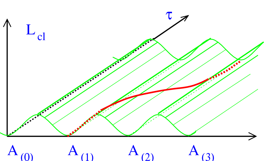
Figure 5: Topological structure of QCD vacuum. The minima correspond to classical ground states with topologically different gauge field configurations $A_{(n)}$. Also shown is an instanton trajectory interpolating between the classical vacua $A_{(1)}$ and $A_{(2)}$. The third axis shows the Euclidean time $\tau$. From hilmar ; courtesy of H. Forkel.

In a quantum theory, however, the system will not stay in one of the minima, like the classical system would. Instead, there will be tunneling processes between different minima. These tunneling processes, in Minkowski space, correspond to instantons. Since tunneling, in general, lowers the ground state energy of the system, one expects the QCD vacuum to have a complicated structure.

Instantons, through the anomaly relation (42), lead to the explicit violation of the $U_{A}(1)$ symmetry and thus solve the mystery of the missing ninth Goldstone boson - the $\eta^{\prime}$. Physically, axial symmetry $U_{A}(1)$ is broken because the tunneling processes between topologically different vacua are accompanied by the change in quark helicity – even in the vacuum, left-handed quarks periodically turn into right-handed and vice versa.

1.2.6 Strong CP problem

The vacuum structure shown in Fig. 5 immediately leads to a puzzle known as the strong CP problem: When one calculates the expectation value of an observable in the vacuum, one has to average over all topological sectors of the vacuum. This is equivalent to adding an additional term to the QCD-Lagrangian,

$${\cal L}_{\rm QCD}\to{\cal L}_{\rm QCD}-\frac{\theta}{16\pi^{2}}\;{\rm tr}\;G^{\mu\nu}\widetilde{G}_{\mu\nu},$$ (43)

where $\theta\in[0,2\pi]$ is a parameter of the theory which has to be determined from experiment. Since the $\theta$-term in Eq. (43) is CP violating, a non-zero value of $\theta$ would have immediate phenomenological consequences, e.g. an electric dipole moment of the neutron. However, precision measurements of this dipole moment constrain $\theta$ to $\theta<10^{-9}$. The fact that $\theta$ is so unnaturally small constitutes the strong CP problem. The most likely solution to this problem axion implies the existence of a light pseudoscalar meson, the axion. However, despite many efforts, axions remain unobserved in experiment.

1.2.7 Phase structure

As was repeatedly stated above, the most important problem facing us in the study of all aspects of QCD is understanding the structure of the vacuum, which, in a manner of saying, does not at all behave as an empty space, but as a physical entity with a complicated structure. As such, the vacuum can be excited, altered and modified in physical processes leewick .

Collisions of heavy ions are the best way to create high energy density in a “macroscopic” (on the scale of a single hadron) volume. It thus could be possible to create and to study a new state of matter, the Quark-Gluon Plasma(QGP), in which quarks and gluons are no longer confined in hadrons, but can propagate freely. The search for QGP is one of the main motivations for the heavy ion research.

Lattice calculations predict that QCD at high temperatures undergoes phase transitions in which confinement property is lost and chiral symmetry is restored. The critical temperature for the chiral phase transition is similar (or maybe even equal) to the critical temperature for deconfinement.

Heavy ion collisions at RHIC may also give us the possibility to study the $\theta$ angle dependence of the QCD phase diagram. In a heavy ion collision, bubbles containing a metastable vacuum with $\theta\neq 0$ may be produced, and reveal themselves through their unusual decay pattern cp .

2 Nuclear interactions at high energies

2.1 Glauber-Gribov Theory

It is intuitively clear that heavy ion collisions are governed by multiple scattering effects. As a short introduction to the basics of multiple scattering theory, we introduce here the eikonal approximation to high energy scattering processes and the Glauber multiple scattering theory Glauber . We also discuss Gribov’s inelastic corrections glaubergribov to Glauber’s theory.

2.1.1 The Eikonal Approximation

The eikonal approximation is the classical approximation to the angular momentum $l$. In partial wave expansion, i.e. in an expansion in angular momentum eigenstates, the scattering amplitude $f(s,t)$ reads ll3

$$f(s,t)=\frac{1}{2{\rm i}p}\sum_{l}(2l+1)\left[{\rm e}^{2{\rm i}\delta_{l}}-1\right]{\rm P}_{l}(\cos\theta),$$ (44)

where $s$ and $t$ are the usual Mandelstam variables (center-of-mass energy squared and invariant momentum transfer, respectively), $p$ is the momentum of the projectile and P_l are the Legendre functions, which depend on the cosine of the scattering angle $\theta$. All information about the interaction is contained in the scattering phases $\delta_{l}$.

High energy scattering is of course a process that is far from being spherically symmetric. Therefore, very large values of $l$ will dominate the sum Eq. (44) and we can treat the angular momentum classically. Since the angular momentum is given by $pb$, one replaces the variable $l$ by the impact parameter $b$,

$$pb=l+\frac{1}{2}.$$ (45)

Note that $b$ is now a continuous variable, so angular momentum is no longer quantized.

At large $l$ and for small scattering angles $\theta$, the Legendre functions can be expressed to good approximation as

$${\rm P}_{l}(\cos\theta)\approx\int_{0}^{2\pi}\frac{d\phi}{2\pi}{\rm e}^{{\rm i}(2l+1)\sin(\theta/2)\cos(\phi)}=\int_{0}^{2\pi}\frac{d\phi}{2\pi}{\rm e}^{{\rm i}\vec{q}\cdot\vec{b}},$$ (46)

where $\vec{q}=\vec{p}-\vec{p}^{\prime}$ is the momentum transfer in the scattering process ($t\approx-|\vec{q}|$) and $|\vec{p}|=|\vec{p}^{\prime}|$ for elastic scattering. At high energy, $\vec{q}$ lies in the impact parameter plane. We have used the relation

$$(2l+1)\sin(\theta/2)\cos(\phi)=2p\sin(\theta/2)\frac{l+1/2}{p}\cos(\phi)=\vec{q}\cdot\vec{b}$$ (47)

to obtain the second equality in Eq. (46).

Thus, the scattering amplitude in eikonal approximation reads

$$f(s,t)=\frac{{\rm i}p}{2\pi}\int d^{2}b{\rm e}^{{\rm i}\vec{q}\cdot\vec{b}}\left[1-{\rm e}^{{\rm i}\chi(s,\vec{b})}\right],$$ (48)

where the phase shift of the projectile is related to the scattering phase $\delta_{l}$ by

$$\chi(s,\vec{b})\equiv 2\delta(s,b).$$ (49)

In the case of scattering off a potential $V(\vec{r})$, this phase shift is simply given by

$$\chi(\vec{b})=-\frac{1}{v}\int_{-\infty}^{\infty}V(\vec{r})dz,$$ (50)

where $v$ is the velocity of the projectile. The scattering amplitude then reads

$$f(s,t)=\frac{{\rm i}p}{2\pi}\int d^{2}b{\rm e}^{{\rm i}\vec{q}\cdot\vec{b}}\left[1-\exp\left(-\frac{{\rm i}}{v}\int V(\vec{r})dz\right)\right].$$ (51)

The total cross section can now be obtained from the forward scattering amplitude via the optical theorem,

$$\sigma_{tot}=\frac{4\pi}{p}{\rm Im}\,f(s,t=0)=2\int d^{2}b\left(1-{\rm Re}\,{\rm e}^{{\rm i}\chi(b)}\right).$$ (52)

For completeness, we also give the expressions for the elastic and inelastic cross sections. The elastic cross section is obtained by squaring the elastic scattering amplitude and integrating over the solid angle,

$$\sigma_{el}=\int d\Omega_{p^{\prime}}\left|f(\theta,\phi)\right|^{2}.$$ (53)

With the approximation $d\Omega_{p^{\prime}}\approx d^{2}p^{\prime}/p^{\prime 2}$, which assumes that scattering takes place predominantly in forward direction, one obtains

$$\sigma_{el}=\int d^{2}b\left|1-{\rm e}^{{\rm i}\chi(b)}\right|^{2}$$ (54)

Finally, the inelastic cross section is

$$\sigma_{inel}=\sigma_{tot}-\sigma_{el}=\int d^{2}b\left(1-\left|{\rm e}^{{\rm i}\chi(b)}\right|^{2}\right).$$ (55)

For potential scattering, the inelastic cross section, of course, vanishes because $\chi(b)$ is real. In general, however, $\chi(b)$ will have an imaginary part.

The expressions Eqs. (52), (54) and (55) could have been obtained directly from the partial wave decomposition of the total, elastic and inelastic cross section, as well. The conditions under which the eikonal approximation is applicable are investigated in detail in Glauber .

2.1.2 Multiple Scattering Theory

Based on the eikonal approximation, it is quite straightforward to develop a theory for scattering off a composite system. In this section, we explain the basic features of the multiple scattering theory developed by Glauber Glauber . A much more detailed presentation of this subject can be found in Glauber .

Assuming that the scatterings on different nucleons are independent, the phase shifts from each scattering simply add up,

$$\chi(\vec{b},\vec{r}_{1},\vec{r}_{2},\dots\vec{r}_{a})=\sum_{j=1}^{A}\chi_{j}(\vec{b}-\vec{s}_{j}).$$ (56)

Here, $\vec{b}$ is the impact parameter of the projectile and $\vec{s}_{j}$, $j=1\dots A$ are the impact parameters of the $A$ nucleons in the nucleus, see Fig. 6.

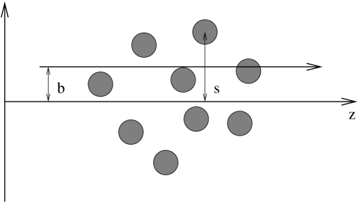
Figure 6: Scattering off a composite system. The impact parameter of the projectile is denoted by $\vec{b}$, while the impact parameters of the scattering centers are denoted by $\vec{s}_{j}$.

The amplitude for scattering off a nuclear target then can be written as

$$F_{fi}^{A} = \frac{{\rm i}p}{2\pi}\int d^{2}b{\rm e}^{{\rm i}\vec{q}\cdot\vec{b}}\langle f|1-\prod_{j=1}^{A}{\rm e}^{{\rm i}\chi_{j}(\vec{b}-\vec{s}_{j})}|i\rangle$$ (57)

$$= \frac{{\rm i}p}{2\pi}\int d^{2}b{\rm e}^{{\rm i}\vec{q}\cdot\vec{b}}\langle f|1-\prod_{j=1}^{A}[1-\gamma_{j}(\vec{b}-\vec{s}_{j})]|i\rangle,$$ (58)

where $|f\rangle$ and $|i\rangle$ are the final and initial state of the target, respectively. In the second step, we introduced the profile function $\gamma(\vec{b})$, which is related to the single-scattering amplitude $f(\vec{q})$ by

$$\gamma(\vec{b})=\frac{1}{2\pi{\rm i}p}\int d^{2}q{\rm e}^{-{\rm i}\vec{q}\cdot\vec{b}}f(\vec{q}).$$ (59)

Thus, we have expressed the nuclear scattering amplitude in terms of the amplitude for scattering off a single nucleon.

In the case of a purely imaginary $f(\vec{q})$, $\gamma(\vec{b})$ is the probability of absorption of the projectile by a nucleon and the nuclear scattering amplitude, Eq. (58) has a simple probabilistic interpretation. Namely, $1-\gamma_{j}(\vec{b}-\vec{s}_{j})$ is the probability of not being absorbed by nucleon number $j$. Taking the product over all $j\in\{1\dots A\}$ yields the probability of not being absorbed by any nucleon in the target. Finally, $1-\prod_{j=1}^{A}[1-\gamma_{j}(\vec{b}-\vec{s}_{j})]$ is the probability that the projectile is absorbed by any of the nucleons.

Also, if one in addition assumes that all nucleons in the target are identical, the nuclear cross section can be expressed in terms of the cross section for scattering on a single nucleon,

$$\sigma_{tot}^{A} = \frac{4\pi}{p}{\rm Im}F_{ii}^{A}(t=0)$$ (60)

$$= 2\int d^{2}b\left(1-\left(1-\frac{\sigma_{tot}^{N}T(\vec{b})}{2A}\right)^{A}\right)$$ (61)

$$\approx 2\int d^{2}b\left(1-\exp\left(-\frac{\sigma_{tot}^{N}T_{A}(\vec{b})}{2}\right)\right),$$ (62)

where the nuclear thickness function $T_{A}(\vec{b})$ is the integral over the nuclear density,

$$T_{A}(\vec{b})=\int_{-\infty}^{\infty}dz\rho_{A}(\vec{b},z).$$ (63)

The simple expression, Eq. (61), resums all multiple scattering terms. We stress that the probabilistic interpretation of Eq. (58) as well as Eqs. (61) and (62) only hold for a purely imaginary $f(\vec{q})$.

The meaning of the nuclear scattering amplitude, Eq. (58), is further explained by expanding the probability of particle absorption by any of the nucleons in powers of $\gamma(\vec{b})$,

$$\Gamma(\vec{b},\vec{r}_{1},\vec{r}_{2},\dots\vec{r}_{a}) \equiv 1-\prod_{j=1}^{A}[1-\gamma_{j}(\vec{b}-\vec{s}_{j})]$$ (64)

$$= \sum_{k=1}^{A}\gamma_{k}(\vec{b}-\vec{s}_{k})-\sum_{k>j}\gamma_{k}(\vec{b}-\vec{s}_{k})\gamma_{j}(\vec{b}-\vec{s}_{j})+\dots\,.$$ (65)

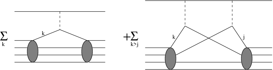
Figure 7: Illustration of the single and double scattering terms in Eq. (65). The coherent sum over all graphs leads to interferences that reduce the total cross section.

The first two terms in this expansion are illustrated in Fig. 7. The first term in Eq. (65) is just the sum of single scattering amplitudes. However, different nucleons in the nucleus compete to interact with the projectile. This effect is contained in the second term in Eq. (65), which reduces the cross section. This reduction is an interference effect that appears because the amplitudes for scattering on different nucleons have to be added coherently. This destructive interference can be observed in experiment as shadowing in hadron-nucleus interactions (eclipse effect in deuterium). Note, however, that shadowing is not completely explained by Glauber theory, as will be explained in the following section.

The easiest application of Glauber multiple scattering theory to nuclear systems is the calculation of the inelastic nucleus-nucleus ($AB$) cross section, which can be written as

$$\sigma_{AB}^{in}=\int d^{2}b(1-P_{0}(b)).$$ (66)

here, $P_{0}(b)$ is the probability that no interaction takes place,

$$P_{0}(b)=(1-\sigma_{NN}^{in}T_{AB}(b))^{AB},$$ (67)

where the nuclear overlap function is given by

$$T_{AB}(\vec{b})=\int d^{2}sT_{A}(\vec{s})T_{B}(\vec{b}-\vec{s}).$$ (68)

(Obviously, $1-P_{0}(b)$ is then the probability of an inelastic interaction, and the meaning of Eq. (66) becomes very transparent.) As it is common, we have labeled the two nuclei by their atomic mass numbers $A$ and $B$.

Another application is the calculation of inclusive particle spectra. With the help of crossing symmetry, the cross section for production of a particle of type $a$ in an $AB$ collision, $AB\to aX$, can be calculated from the total cross section of the process $\bar{a}AB\to X$, where $\bar{a}$ is the antiparticle of $a$. According to so-called AGK cutting rules agk , the nuclear cross section for this process is given by

$$E\frac{d^{3}\sigma^{a}_{AB}}{d^{2}bd^{3}p}=T_{AB}(\vec{b})E\frac{d^{3}\sigma^{a}_{NN}}{d^{3}p}.$$ (69)

Integration over impact parameter $b$ yields

$$E\frac{d^{3}\sigma^{a}_{AB}}{d^{3}p}=AB\;E\frac{d^{3}\sigma^{a}_{NN}}{d^{3}p},$$ (70)

and correspondingly the charged particle multiplicity would scale proportional to $AB$,

$$\frac{dn_{ch}}{d\eta}=AB\;\frac{1}{\sigma^{in}_{AB}}\frac{d\sigma^{ch}_{NN}}{d\eta},$$ (71)

the meaning of which is obvious – if collisions are truly independent, the resulting multiplicity should scale with the number of collisions, $AB$.

However, the relation (71) appears to be badly violated in experiment. What went wrong? It appears that the disagreement between the result Eq. (71) and experimental data is due to the fact that there are important corrections to the Glauber multiple scattering theory, which we neglected so far. These corrections are known as Gribov’s inelastic shadowing glaubergribov and will be the subject of the next section.

2.1.3 Gribov’s “Inelastic Shadowing”

The assumed independence of nucleon–nucleon collisions is violated by the diagrams of the type of Fig. 8, where the projectile is excited into a state $|n\rangle$ by the interaction. The diagram in Fig. 8 does not describe independent collisions, and at high energies it will interfere with the double scattering graph in Fig. 7.

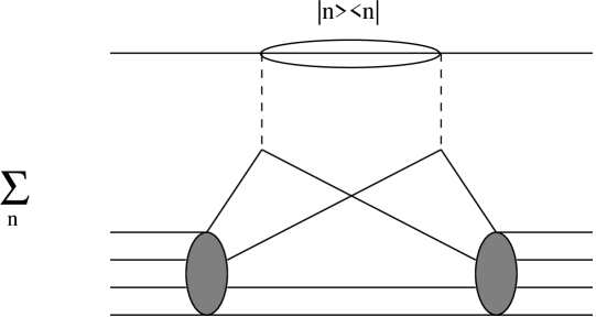
Figure 8: If the projectile is a composite particle, it can be excited by the interaction. Therefore, this graph will interfere with the double scattering graph in Fig. 7.

The excitation of an inelastic state in the scattering is accompanied by a longitudinal momentum transfer

$$\Delta p_{L}=\frac{M_{f}^{2}-M_{i}^{2}}{2p},$$ (72)

where $M_{f}$ is the invariant mass of the excited system and $M_{i}$ is the invariant mass of the projectile in the initial state. The diagram in Fig. 8 is only important if it can make a significant contribution to the forward scattering amplitude $F^{A}_{ii}$. This requires that the longitudinal momentum transfer must be so small that the nucleus has a chance to remain intact, i.e.

$$\Delta p_{L}R_{A}\mathrel{\hbox to0.0pt{\lower 4.0pt\hbox{\hskip 1.0pt$\sim$}\hss}\raise 1.0pt\hbox{$<$}}1,$$ (73)

where $R_{A}$ is the nuclear radius. Apparently, this condition is fulfilled for sufficiently large values of the projectile momentum $p$ in Eq. (72). Thus, as it was first found by Gribov in glaubergribov , Glauber theory receives important corrections at high energy.

The condition, Eq. (73), which determines, whether Gribov’s inelastic shadowing becomes relevant, leads us to the important quantum mechanical concept of formation time, or formation length. The formation time is the lifetime of the excitation $|n\rangle$ in Fig. 8 in the target rest frame and the formation length is the longitudinal distance over which the excited state $|n\rangle$ lives. At high energy, of course, both quantities are identical. The formation time/length can be determined in a time-dependent and in a time-independent approach.

In the time dependent formulation, one starts from the energy-time uncertainty relation,

$$\Delta E\Delta t\mathrel{\hbox to0.0pt{\lower 4.0pt\hbox{\hskip 1.0pt$\sim$}\hss}\raise 1.0pt\hbox{$>$}}1.$$ (74)

The lifetime of the excitation in rest frame of the projectile is given by

$$\tau_{f}\approx\frac{1}{M_{f}-M_{i}}.$$ (75)

In order to obtain the formation time, we have to transform $\tau_{f}$ to the target rest frame, by multiplying $\tau_{f}$ with the relativistic $\gamma$-factor,

$$t_{f}\equiv\Delta t=\gamma\tau_{f}=\frac{p}{\bar{M}}\tau_{f},$$ (76)

where

$$\bar{M}=\frac{M_{f}+M_{i}}{2}.$$ (77)

We finally obtain for the formation time

$$t_{f}\approx\frac{2p}{M_{f}^{2}-M_{i}^{2}}.$$ (78)

In the time-independent approach, one starts from the coordinate-momentum uncertainty relation,

$$\Delta p_{L}\Delta z\mathrel{\hbox to0.0pt{\lower 4.0pt\hbox{\hskip 1.0pt$\sim$}\hss}\raise 1.0pt\hbox{$>$}}1.$$ (79)

The longitudinal momentum transfer was already given in Eq. 72. It is calculated in the following way,

$$\Delta p_{L}=\sqrt{E^{2}-M_{i}^{2}}-\sqrt{E^{2}-M_{f}^{2}}\approx\frac{M_{f}^{2}-M_{i}^{2}}{2p}.$$ (80)

According to the uncertainty relation Eq. (79), the excited state lives over the longitudinal extension

$$l_{f}\equiv\Delta z\approx\frac{1}{\Delta p_{L}}\approx\frac{2p}{M_{f}^{2}-M_{i}^{2}}.$$ (81)

As expected, the formation length is identical to the formation time given in Eq. (78).

We see from Eqs. (78) and (81) that for large initial projectile momentum, the process develops at large longitudinal distances in the target rest frame. At the high center of mass energies of RHIC and LHC, the coherence length will be much larger than the nuclear radius and all scattering processes will be governed by coherence effects (the coherence length becomes as long as several hundreds fm).

2.2 Elementary hadron–hadron scattering at high energies

All of the formalism presented above is completely independent of the underlying interaction. Before concluding this section, we will briefly discuss the main properties of hadron–hadron scattering at high energies. Let us begin by listing some empirical facts about hadronic cross sections:

• Total hadronic cross sections are approximately constant at cm energies of order $\sqrt{s}\sim 20\,\mbox{GeV}$ and slowly rise, $\sigma_{tot}\sim s^{0.08}$, up to the highest energies accessible in experiment (Tevatron energy, $\sqrt{s}=1.8$ TeV).

• The diffraction cone shrinks as energy increases, indicating that the size of the hadron increases with energy.

• The mean transverse momentum of produced particles is approximately constant or increases only slowly with energy, respectively.

The (approximate) constancy of the total cross section in the framework of QCD implies that high energy hadronic scattering is dominated by two gluon exchange low , see Fig. 9 (left). The two gluon exchange model also yields a purely imaginary forward scattering amplitude. In order to explain the increase of the total cross section with energy, one has to take the radiation of additional gluons into account, see Fig. 9 (right). The probability of gluon emission is proportional to $\alpha_{s}y\sim\alpha_{s}\ln s$, where $y$ is rapidity. Thus, each gluon radiation in Fig. 9 (right) contributes a factor $\ln s$ to the total cross section. Resumming an infinite number of gluon emissions ordered in rapidity, one finds that the total cross section behaves like

$$\sigma_{tot}\propto\sum_{n}\frac{(\ln s)^{n}}{n!}a^{n}=s^{a},$$ (82)

where $a\propto\alpha_{s}$.

Figure 9: Double gluon exchange (left), yields an imaginary scattering amplitude and a constant cross section. The rise of hadronic cross sections and the shrinkage of the diffraction cone at high energy is due to radiation of additional gluons (right).

This gluon radiation also explains the shrinkage of the diffraction cone. At high energy, the $t$-differential cross section in hadronic collisions behaves like

$$\frac{d\sigma}{dt}=\left.\frac{d\sigma}{dt}\right|_{t=0}{\rm e}^{-B(s)|t|},$$ (83)

where $B(s)\propto\ln s$ increases with energy. Such a behavior emerges, if the elastic scattering amplitude in impact parameter space is given by

$$f_{el}\propto\exp\left(\frac{b}{R^{2}_{h}(s)}\right),$$ (84)

where the effective hadron radius $R^{2}_{h}(s)$ increases as a function of energy. Therefore, the shrinkage of the diffraction peak suggests an increase of hadronic sizes with energy. In QCD, this can be understood in the following way: Gluons are radiated off the projectile with different transverse momenta. As rapidity, or energy, increases, these gluons perform a random walk in the impact parameter plane and correspondingly, the transverse size of the gluon cloud surrounding the projectile increases. This can be regarded as a diffusion process in the impact parameter plane, in which rapidity plays the role of time.

The slow increase of the mean transverse momentum with energy is likely to be related to asymptotic freedom. Indeed, at large transverse momentum, $p_{\perp}\gg\Lambda_{QCD}$, the strong coupling constant becomes small, $\alpha_{s}(p_{\perp})\ll 1$, which suppresses the production of high $p_{\perp}$ particles.

Eventually, the power-like growth of the total hadronic cross section will violate the Froissart-Martin bound froissart , which states that as a consequence of unitarity and analyticity, total cross sections cannot rise faster than

$$\sigma_{tot}\mathrel{\hbox to0.0pt{\lower 4.0pt\hbox{\hskip 1.0pt$\sim$}\hss}\raise 1.0pt\hbox{$<$}}C\ln^{2}s,$$ (85)

where $C$ is a constant. At sufficiently high energy, emitted gluons can develop showers themselves, see Fig. 10. Due to this process, the projectile sees a reduced gluon density in the target and the growth of the cross section is slowed down. This effect, in the squared amplitude, realizes a QCD realization of Gribov’s inelastic shadowing (see Fig. 10.) Even though such unitarity corrections might already be present in proton-antiproton scattering at Tevatron, they will be much more pronounced in nuclear collisions at RHIC.

Figure 10: At sufficiently high energy, emitted gluons can themselves develop showers. In the squared amplitude (right), the gluons combine to ladders, which are denoted by zigzag lines. Fusion of gluon ladders is the mechanism behind gluon shadowing. A resummation of fan diagrams like in the left figure, corresponds to classical solutions schwimmer of Reggeon Field Theory reggeonfield .

As the magnitude of these effects increases with energy and/or atomic number of the colliding nuclei, the classification of diagrams in terms of individual nucleon–nucleon amplitudes (or parton ladders) rapidly starts to lose sense – the non–linear effects become extremely important. The treatment of nuclear interactions in this high–density regime will be considered in the following section.

3 Classical Chromodynamics of Relativistic Heavy Ion Collisions

3.1 QCD in the classical regime

Most of the applications of QCD so far have been limited to the short distance regime of high momentum transfer, where the theory becomes weakly coupled and can be linearized. While this is the only domain where our theoretical tools based on perturbation theory are adequate, this is also the domain in which the beautiful non–linear structure of QCD does not yet reveal itself fully. On the other hand, as soon as we decrease the momentum transfer in a process, the dynamics rapidly becomes non–linear, but our understanding is hindered by the large coupling. Being perplexed by this problem, one is tempted to dream about an environment in which the coupling is weak, allowing a systematic theoretical treatment, but the fields are strong, revealing the full non–linear nature of QCD. We are going to argue now that this environment can be created on Earth with the help of relativistic heavy ion colliders. Relativistic heavy ion collisions allow to probe QCD in the non–linear regime of high parton density and high color field strength, see Fig. 11.

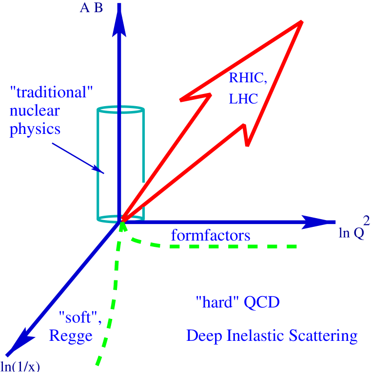
Figure 11: The place of relativistic heavy ion physics in the study of QCD; the vertical axis is the product of atomic numbers of projectile and target, and the horizontal axes are the momentum transfer $Q^{2}$ and rapidity $y=\ln(1/x)$ ($x$ is the Bjorken scaling variable).

It has been conjectured long time ago that the dynamics of QCD in the high density domain may become qualitatively different: in parton language, this is best described in terms of parton saturation Gribov, Levin and Ryskin (1983); Mueller and Qiu (1986); Blaizot and Mueller (1987), and in the language of color fields – in terms of the classical Chromo–Dynamics McLerran and Venugopalan (1994); see the lectures Iancu, Leonidov, McLerran (2002) and Mueller (2001) and references therein. In this high density regime, the transition amplitudes are dominated not by quantum fluctuations, but by the configurations of classical field containing large, $\sim 1/\alpha_{s}$, numbers of gluons. One thus uncovers new non–linear features of QCD, which cannot be investigated in the more traditional applications based on the perturbative approach. The classical color fields in the initial nuclei (the “color glass condensate” Iancu, Leonidov, McLerran (2002)) can be thought of as either perturbatively generated, or as being a topologically non–trivial superposition of the Weizsäcker-Williams radiation and the quasi–classical vacuum fields Kharzeev, Kovchegov and Levin (2001); Nowak, Shuryak and Zahed (2001); Kharzeev, Kovchegov and Levin (2002).

3.1.1 Geometrical arguments

Let us consider an external probe $J$ interacting with the nuclear target of atomic number $A$. At small values of Bjorken $x$, by uncertainty principle the interaction develops over large longitudinal distances $z\sim 1/mx$, where $m$ is the nucleon mass. As soon as $z$ becomes larger than the nuclear diameter, the probe cannot distinguish between the nucleons located on the front and back edges of the nucleus, and all partons within the transverse area $\sim 1/Q^{2}$ determined by the momentum transfer $Q$ participate in the interaction coherently. The density of partons in the transverse plane is given by

$$\rho_{A}\simeq{xG_{A}(x,Q^{2})\over\pi R_{A}^{2}}\sim A^{1/3},$$ (86)

where we have assumed that the nuclear gluon distribution scales with the number of nucleons $A$. The probe interacts with partons with cross section $\sigma\sim\alpha_{s}/Q^{2}$; therefore, depending on the magnitude of momentum transfer $Q$, atomic number $A$, and the value of Bjorken $x$, one may encounter two regimes:

• $\sigma\rho_{A}\ll 1$ – this is a familiar “dilute” regime of incoherent interactions, which is well described by the methods of perturbative QCD;

• $\sigma\rho_{A}\gg 1$ – in this regime, we deal with a dense parton system. Not only do the “leading twist” expressions become inadequate, but also the expansion in higher twists, i.e. in multi–parton correlations, breaks down here.

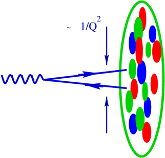
Figure 12: Hard probe interacting with the nuclear target resolves the transverse distance $\sim 1/\sqrt{Q}$ ($Q^{2}$ is the square of the momentum transfer) and, in the target rest frame, the longitudinal distance $\sim 1/(mx)$ ($m$ is the nucleon mass and $x$ the Bjorken variable).

The border between the two regimes can be found from the condition $\sigma\rho_{A}\simeq 1$; it determines the critical value of the momentum transfer (“saturation scale”Gribov, Levin and Ryskin (1983)) at which the parton system becomes to look dense to the probe:

$$Q_{s}^{2}\sim\alpha_{s}\ {xG_{A}(x,Q_{s}^{2})\over\pi R_{A}^{2}}.$$ (87)

In this regime, the number of gluons from (87) is given by

$$xG_{A}(x,Q_{s}^{2})\sim{\pi\over\alpha_{s}(Q_{s}^{2})}\ Q_{s}^{2}R_{A}^{2},$$ (88)

where $Q_{s}^{2}R_{A}^{2}\sim A$. One can see that the number of gluons is proportional to the inverse of $\alpha_{s}(Q_{s}^{2})$, and becomes large in the weak coupling regime. In this regime, as we shall now discuss, the dynamics is likely to become essentially classical.

3.1.2 Saturation as the classical limit of QCD

Indeed, the condition (87) can be derived in the following, rather general, way. As a first step, let us note that the dependence of the action corresponding to the Lagrangian (9) on the coupling constant is given by

$$S\sim\int{1\over g^{2}}\ G_{\mu\nu}^{a}G_{\mu\nu}^{a}\ d^{4}x.$$ (89)

Let us now consider a classical configuration of gluon fields; by definition, $G_{\mu\nu}^{a}$ in such a configuration does not depend on the coupling, and the action is large, $S\gg\hbar$. The number of quanta in such a configuration is then

$$N_{g}\sim{S\over\hbar}\sim{1\over\hbar\ g^{2}}\ \rho_{4}V_{4},$$ (90)

where we re-wrote (89) as a product of four–dimensional action density $\rho_{4}$ and the four–dimensional volume $V_{4}$.

Note that since (90) depends only on the product of the Planck constant $\hbar$ and the coupling $g^{2}$, the classical limit $\hbar\to 0$ is indistinguishable from the weak coupling limit $g^{2}\to 0$. The weak coupling limit of small $g^{2}=4\pi\alpha_{s}$ therefore corresponds to the semi–classical regime.

The effects of non–linear interactions among the gluons become important when $\partial_{\mu}A_{\mu}\sim A_{\mu}^{2}$ (this condition can be made explicitly gauge invariant if we derive it from the expansion of a correlation function of gauge-invariant gluon operators, e.g., $G^{2}$). In momentum space, this equality corresponds to

$$Q_{s}^{2}\sim(A_{\mu})^{2}\sim(G^{2})^{1/2}=\sqrt{\rho_{4}};$$ (91)

$Q_{s}$ is the typical value of the gluon momentum below which the interactions become essentially non–linear.

Consider now a nucleus $A$ boosted to a high momentum. By uncertainty principle, the gluons with transverse momentum $Q_{s}$ are extended in the longitudinal and proper time directions by $\sim 1/Q_{s}$; since the transverse area is $\pi R_{A}^{2}$, the four–volume is $V_{4}\sim\pi R_{A}^{2}/Q_{s}^{2}$. The resulting four–density from (90) is then

$$\rho_{4}\sim\alpha_{s}\ {N_{g}\over V_{4}}\sim\alpha_{s}\ {N_{g}\ Q_{s}^{2}\over\pi R_{A}^{2}}\sim Q_{s}^{4},$$ (92)

where at the last stage we have used the non–linearity condition (91), $\rho_{4}\sim Q_{s}^{4}$. It is easy to see that (92) coincides with the saturation condition (87), since the number of gluons in the infinite momentum frame $N_{g}\sim xG(x,Q_{s}^{2})$.

In view of the significance of saturation criterion for the rest of the material in these lectures, let us present yet another argument, traditionally followed in the discussion of classical limit in electrodynamics Berestetskii,Lifshitz and Pitaevskii (1982). The energy of the gluon field per unit volume is $\sim\vec{E}^{a2}$. The number of elementary “oscillators of the field”, also per unit volume, is $\sim\omega^{3}$. To get the number of the quanta in the field we have to divide the energy of the field by the product of the number of the oscillators $\sim\omega^{3}$ and the average energy $\hbar\omega$ of the gluon:

$$N_{{\vec{k}}}\sim{\vec{E}^{a2}\over\hbar\omega^{4}}.$$ (93)

The classical approximation holds when $N_{{\vec{k}}}\gg 1$. Since the energy $\omega$ of the oscillators is related to the time $\Delta t$ over which the average energy is computed by $\omega\sim 1/\Delta t$, we get

$$\vec{E}^{a2}\gg{\hbar\over(\Delta t)^{4}}.$$ (94)

Note that the quantum mechanical uncertainty principle for the energy of the field reads

$$\vec{E}^{a2}\ \omega^{4}\sim\hbar,$$ (95)

so the condition (94) indeed defines the quasi–classical limit.

Since $\vec{E}^{a2}$ is proportional to the action density $\rho_{4}$, and the typical time is $\Delta t\sim 1/k_{\perp}$, using (92) we finally get that the classical description applies when

$$k_{\perp}^{2}<\alpha_{s}{N_{g}\over\pi R_{A}^{2}}\equiv Q_{s}^{2}.$$ (96)

3.1.3 The absence of mini–jet correlations

When the occupation numbers of the field become large, the matrix elements of the creation and annihilation operators of the gluon field defined by

$$\hat{A}^{\mu}=\sum_{\vec{k},\alpha}(\hat{c}_{\vec{k}\alpha}A^{\mu}_{\vec{k}\alpha}+\hat{c}^{\dagger}_{\vec{k}\alpha}A^{\mu*}_{\vec{k}\alpha})$$ (97)

become very large,

$$N_{\vec{k}\alpha}=\langle\hat{c}^{\dagger}_{\vec{k}\alpha}\hat{c}_{\vec{k}\alpha}\rangle\gg 1,$$ (98)

so that one can neglect the unity on the r.h.s. of the commutation relation

$$\hat{c}_{\vec{k}\alpha}\hat{c}^{\dagger}_{\vec{k}\alpha}-\hat{c}^{\dagger}_{\vec{k}\alpha}\hat{c}_{\vec{k}\alpha}=1$$ (99)

and treat these operators as classical $c-$numbers.

This observation, often used in condensed matter physics, especially in the theoretical treatment of superfluidity, has important consequences for gluon production – in particular, it implies that the correlations among the gluons in the saturation region can be neglected:

$$\langle A(k_{1})A(k_{2})...A(k_{n})\rangle\simeq\langle A(k_{1})\rangle\langle A(k_{2})\rangle...\langle A(k_{n})\rangle.$$ (100)

Thus, in contrast to the perturbative picture, where the produced mini-jets have strong back-to-back correlations, the gluons resulting from the decay of the classical saturated field are uncorrelated at $k_{\perp}\mathrel{\hbox to0.0pt{\lower 4.0pt\hbox{\hskip 1.0pt$\sim$}\hss}\raise 1.0pt\hbox{$<$}}Q_{s}$.

Note that the amplitude with the factorization property (100) is called point–like. However, the relation (100) cannot be exact if we consider the correlations of final–state hadrons – the gluon mini–jets cannot transform into hadrons independently. These correlations caused by color confinement however affect mainly hadrons with close three–momenta, as opposed to the perturbative correlations among mini–jets with the opposite three–momenta.

It will be interesting to explore the consequences of the factorization property of the classical gluon field (100) for the HBT correlations of final–state hadrons. It is likely that the HBT radii in this case reflect the universal color correlations in the hadronization process.

Another interesting property of classical fields follows from the relation

$$\langle(\hat{c}^{\dagger}_{\vec{k}\alpha}\hat{c}_{\vec{k}\alpha})^{2}\rangle-\langle\hat{c}^{\dagger}_{\vec{k}\alpha}\hat{c}_{\vec{k}\alpha}\rangle^{2}=\langle\hat{c}^{\dagger}_{\vec{k}\alpha}\hat{c}_{\vec{k}\alpha}\rangle,$$ (101)

which determines the fluctuations in the number of produced gluons. We will discuss the implications of Eq. (101) for the multiplicity fluctuations in heavy ion collisions later.

3.2 Classical QCD in action

3.2.1 Centrality dependence of hadron production

In nuclear collisions, the saturation scale becomes a function of centrality; a generic feature of the quasi–classical approach – the proportionality of the number of gluons to the inverse of the coupling constant (90) – thus leads to definite predictions Kharzeev and Nardi (2001) on the centrality dependence of multiplicity.

Let us first present the argument on a qualitative level. At different centralities (determined by the impact parameter of the collision), the average density of partons (in the transverse plane) participating in the collision is very different. This density $\rho$ is proportional to the average length of nuclear material involved in the collision, which in turn approximately scales with the power of the number $N_{part}$ of participating nucleons, $\rho\sim N_{part}^{1/3}$. The density of partons defines the value of the saturation scale, and so we expect

$$Q_{s}^{2}\sim N_{part}^{1/3}.$$ (102)

The gluon multiplicity is then, as we discussed above, is

$${dN_{g}\over d\eta}\sim{S_{A}\ Q_{s}^{2}\over\alpha_{s}(Q_{s}^{2})},$$ (103)

where $S_{A}$ is the nuclear overlap area, determined by atomic number and the centrality of collision. Since $S_{A}\ Q_{s}^{2}\sim N_{part}$ by definitions of the transverse density and area, from (103) we get

$${dN_{g}\over d\eta}\sim N_{part}\ \ln N_{part},$$ (104)

which shows that the gluon multiplicity shows a logarithmic deviation from the scaling in the number of participants.

To quantify the argument, we need to explicitly evaluate the average density of partons at a given centrality. This can be done by using Glauber theory, which allows to evaluate the differential cross section of the nucleus–nucleus interactions. The shape of the multiplicity distribution at a given (pseudo)rapidity $\eta$ can then be readily obtained by using the formulae introduced in section 2:

$$\frac{d\sigma}{dn}=\int d^{2}b\ {\cal P}(n;b)\ (1-P_{0}(b)),$$ (105)

where $P_{0}(b)$ is the probability of no interaction among the nuclei at a given impact parameter $b$:

$$P_{0}(b)=(1-\sigma_{NN}T_{AB}(b))^{AB};$$ (106)

$\sigma_{NN}$ is the inelastic nucleon–nucleon cross section, and $T_{AB}(b)$ is the nuclear overlap function for the collision of nuclei with atomic numbers A and B; we have used the three–parameter Woods–Saxon nuclear density distributions De Jager, De Vries and De Vries (1974).

The correlation function ${\cal P}(n;b)$ is given by

$${\cal P}(n;b)=\frac{1}{\sqrt{2\pi a\bar{n}(b)}}\ \exp\left(-\frac{(n-\bar{n}(b))^{2}}{2a\bar{n}(b)}\right),$$ (107)

here $\bar{n}(b)$ is the mean multiplicity at a given impact parameter $b$; the formulae for the number of participants and the number of binary collisions can be found in Kharzeev, Lourenço, Nardi and Satz (1997). The parameter $a$ describes the strength of fluctuations; for the classical gluon field, as follows from (101), $a=1$. However, the strength of fluctuations can be changed by the subsequent evolution of the system and by hadronization process. Moreover, in a real experiment, the strength of fluctuations strongly depends on the acceptance. In describing the PHOBOS distribution PHOBOS Coll. (2000), we have found that the value $a=0.6$ fits the data well.

In Fig. 13, we compare the resulting distributions for two different assumptions about the scaling of multiplicity with the number of participants to the PHOBOS experimental distribution, measured in the interval $3<|\eta|<4.5$. One can see that almost independently of theoretical assumptions about the dynamics of multiparticle production, the data are described quite well. At first this may seem surprising; the reason for this result is that at high energies, heavy nuclei are almost completely “black”; unitarity then implies that the shape of the cross section is determined almost entirely by the nuclear geometry. We can thus use experimental differential cross sections as a reliable handle on centrality. This gives us a possibility to compute the dependence of the saturation scale on centrality of the collision, and thus to predict the centrality dependence of particle multiplicities, shown in Fig. 14. (see Kharzeev and Nardi (2001) for details).

Figure 13: Charged multiplicity distribution at $\sqrt{s}=130$ A GeV; solid line (histogram) – PHOBOS result; dashed line – distribution corresponding to participant scaling ($x=0$); dotted line – distribution corresponding to the $37\%$ admixture of “hard” component in the multiplicity; see text for details.

Figure 14: Centrality dependence of the charged multiplicity per participant pair near $\eta=0$ at $\sqrt{s}=130$ A GeV; the curves represent the prediction based on the conventional eikonal approach, while the diamonds correspond to the high density QCD prediction (see text). The square indicates the $pp$ multiplicity.

3.2.2 Energy dependence

Let us now turn to the discussion of energy dependence of hadron production. In semi–classical scenario, it is determined by the variation of saturation scale $Q_{s}$ with Bjorken $x=Q_{s}/\sqrt{s}$. This variation, in turn, is determined by the $x-$ dependence of the gluon structure function. In the saturation approach, the gluon distribution is related to the saturation scale by Eq.(87). A good description of HERA data is obtained with saturation scale $Q_{s}^{2}=1\div 2\ \rm{GeV}^{2}$ with $W$ - dependence ($W\equiv\sqrt{s}$ is the center-of-mass energy available in the photon–nucleon system) Golec-Biernat and Wüsthoff (1999)

$$Q^{2}_{s}\,\,\propto\,W^{\lambda},$$ (108)

where $\lambda\simeq 0.25\div 0.3$. In spite of significant uncertainties in the determination of the gluon structure functions, perhaps even more important is the observation Golec-Biernat and Wüsthoff (1999) that the HERA data exhibit scaling when plotted as a function of variable

$$\tau\,=\,{Q^{2}\over Q_{0}^{2}}\ \left({x\over x_{0}}\right)^{\lambda},$$ (109)

where the value of $\lambda$ is again within the limits $\lambda\simeq 0.25\div 0.3$. In high density QCD, this scaling is a consequence of the existence of dimensionful scale Gribov, Levin and Ryskin (1983); McLerran and Venugopalan (1994)

$$Q_{s}^{2}(x)=Q_{0}^{2}\ (x_{0}/x)^{\lambda}.$$ (110)

Using the value of $Q_{s}^{2}\simeq 2.05\ {\rm GeV}^{2}$ extracted Kharzeev and Nardi (2001) at $\sqrt{s}=130$ GeV and $\lambda=0.25$ Golec-Biernat and Wüsthoff (1999) used in Kharzeev and Levin (2000), equation (120) leads to the following approximate formula for the energy dependence of charged multiplicity in central $Au-Au$ collisions:

$$\left<{2\over N_{part}}\ {dN_{ch}\over d\eta}\right>_{\eta<1}\approx 0.87\ \left({\sqrt{s}\ ({\rm GeV})\over 130}\right)^{0.25}\ \times$$

$$\times\left[3.93+0.25\ \ln\left({\sqrt{s}\ ({\rm GeV})\over 130}\right)\right].$$ (111)

At $\sqrt{s}=130\ {\rm GeV}$, we estimate from Eq.(111) $2/N_{part}\ dN_{ch}/d\eta\mid_{\eta<1}=3.42\pm 0.15$, to be compared to the average experimental value of $3.37\pm 0.12$ PHOBOS Coll. (2000); PHENIX Coll. (2001); STAR Coll. (2001); BRAHMS Coll. (2001). At $\sqrt{s}=200\ {\rm GeV}$, one gets $3.91\pm 0.15$, to be compared to the PHOBOS value PHOBOS Coll. (2000) of $3.78\pm 0.25$. Finally, at $\sqrt{s}=56\ {\rm GeV}$, we find $2.62\pm 0.15$, to be compared to PHOBOS Coll. (2000) $2.47\pm 0.25$. It is interesting to note that formula (111), when extrapolated to very high energies, predicts for the LHC energy a value substantially smaller than found in other approaches:

$$\left<{2\over N_{part}}\ {dN_{ch}\over d\eta}\right>_{\eta<1}=10.8\pm 0.5;\ \ \ \sqrt{s}=5500\ {\rm GeV},$$ (112)

corresponding only to a factor of $2.8$ increase in multiplicity between the RHIC energy of $\sqrt{s}=200\ {\rm GeV}$ and the LHC energy of $\sqrt{s}=5500\ {\rm GeV}$ (numerical calculations show that when normalized to the number of participants, the multiplicity in central $Au-Au$ and $Pb-Pb$ systems is almost identical). The energy dependence of charged hadron multiplicity per participant pair is shown in Fig.15.

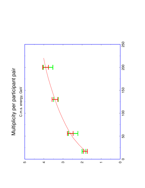
Figure 15: Energy dependence of charged multiplicity per participant pair at RHIC energies; solid line is the result (111).

One can also try to extract the value of the exponent $\lambda$ from the energy dependence of hadron multiplicity measured by PHOBOS at $\sqrt{s}=130\ \rm{GeV}$ and at $\sqrt{s}=56\ \rm{GeV}$; this procedure yields $\lambda\simeq 0.37$, which is larger than the value inferred from the HERA data (and is very close to the value $\lambda\simeq 0.38$, resulting from the final–state saturation calculations Eskola, Kajantie, Ruuskanen and Tuominen (2000)).

3.2.3 Radiating the classical glue

Let us now proceed to the quantitative calculation of the (pseudo-) rapidity and centrality dependences Kharzeev and Levin (2001). We need to evaluate the leading tree diagram describing emission of gluons on the classical level, see Fig. 16.

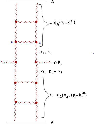
Figure 16: The Mueller diagram for the classical gluon radiation.

Let us introduce the unintegrated gluon distribution $\varphi_{A}(x,k_{t}^{2})$ which describes the probability to find a gluon with a given $x$ and transverse momentum $k_{t}$ inside the nucleus $A$. As follows from this definition, the unintegrated distribution is related to the gluon structure function by

$$xG_{A}(x,p_{t}^{2})=\int^{p_{t}^{2}}dk_{t}^{2}\ \varphi_{A}(x,k_{t}^{2});$$ (113)

when $p_{t}^{2}>Q_{s}^{2}$, the unintegrated distribution corresponding to the bremsstrahlung radiation spectrum is

$$\varphi_{A}(x,k_{t}^{2})\sim{\alpha_{s}\over\pi}\ {1\over k_{t}^{2}}.$$ (114)

In the saturation region, the gluon structure function is given by (88); the corresponding unintegrated gluon distribution has only logarithmic dependence on the transverse momentum:

$$\varphi_{A}(x,k_{t}^{2})\sim{S_{A}\over\alpha_{s}};\ k_{t}^{2}\leq Q_{s}^{2},$$ (115)

where $S_{A}$ is the nuclear overlap area, determined by the atomic numbers of the colliding nuclei and by centrality of the collision.

The differential cross section of gluon production in a $AA$ collision can now be written down as Gribov, Levin and Ryskin (1983); Gyulassy and McLerran (1997)

$$E{d\sigma\over d^{3}p}={4\pi N_{c}\over N_{c}^{2}-1}\ {1\over p_{t}^{2}}\ \int dk_{t}^{2}\ \alpha_{s}\ \varphi_{A}(x_{1},k_{t}^{2})\ \varphi_{A}(x_{2},(p-k)_{t}^{2}),$$ (116)

where $x_{1,2}=(p_{t}/\sqrt{s})\exp(\pm\eta)$, with $\eta$ the (pseudo)rapidity of the produced gluon; the running coupling $\alpha_{s}$ has to be evaluated at the scale $Q^{2}=max\{k_{t}^{2},(p-k)_{t}^{2}\}$. The rapidity density is then evaluated from (116) according to

$${dN\over dy}={1\over\sigma_{AA}}\ \int d^{2}p_{t}\left(E{d\sigma\over d^{3}p}\right),$$ (117)

where $\sigma_{AA}$ is the inelastic cross section of nucleus–nucleus interaction.

Since the rapidity $y$ and Bjorken variable are related by $\ln 1/x=y$, the $x-$ dependence of the gluon structure function translates into the following dependence of the saturation scale $Q_{s}^{2}$ on rapidity:

$$Q_{s}^{2}(s;\pm y)=Q_{s}^{2}(s;y=0)\ \exp(\pm\lambda y).$$ (118)

As it follows from (118), the increase of rapidity at a fixed $W\equiv\sqrt{s}$ moves the wave function of one of the colliding nuclei deeper into the saturation region, while leading to a smaller gluon density in the other, which as a result can be pushed out of the saturation domain. Therefore, depending on the value of rapidity, the integration over the transverse momentum in Eqs. (116),(117) can be split in two regions: i) the region $\Lambda_{QCD}<k_{t}<Q_{s,min}$ in which the wave functions are both in the saturation domain; and ii) the region $\Lambda<<Q_{s,min}<k_{t}<Q_{s,max}$ in which the wave function of one of the nuclei is in the saturation region and the other one is not. Of course, there is also the region of $k_{t}>Q_{s,max}$, which is governed by the usual perturbative dynamics, but our assumption here is that the rôle of these genuine hard processes in the bulk of gluon production is relatively small; in the saturation scenario, these processes represent quantum fluctuations above the classical background. It is worth commenting that in the conventional mini–jet picture, this classical background is absent, and the multi–particle production is dominated by perturbative processes. This is the main physical difference between the two approaches; for the production of particles with $p_{t}>>Q_{s}$ they lead to identical results.

To perform the calculation according to (117),(116) away from $y=0$ we need also to specify the behavior of the gluon structure function at large Bjorken $x$ (and out of the saturation region). At $x\to 1$, this behavior is governed by the QCD counting rules, $xG(x)\sim(1-x)^{4}$, so we adopt the following conventional form: $xG(x)\sim x^{-\lambda}\ (1-x)^{4}$.

We now have everything at hand to perform the integration over transverse momentum in (117), (116); the result is the following Kharzeev and Levin (2001):

$${dN\over dy}=const\ S_{A}\ Q_{s,min}^{2}\ \ln\left({Q_{s,min}^{2}\over\Lambda_{QCD}^{2}}\right)\ \times$$

$$\times\ \left[1+{1\over 2}\ \ln\left({Q_{s,max}^{2}\over Q_{s,min}^{2}}\right)\ \left(1-{Q_{s,max}\over\sqrt{s}}e^{|y|}\right)^{4}\right],$$ (119)

where the constant is energy–independent, $S_{A}$ is the nuclear overlap area, $Q_{s}^{2}\equiv Q_{s}^{2}(s;y=0)$, and $Q_{s,min(max)}$ are defined as the smaller (larger) values of (118); at $y=0$, $Q_{s,min}^{2}=Q_{s,max}^{2}=Q_{s}^{2}(s)=Q_{s}^{2}(s_{0})\ \times(s/s_{0})^{\lambda/2}$. The first term in the brackets in (119) originates from the region in which both nuclear wave functions are in the saturation regime; this corresponds to the familiar $\sim(1/\alpha_{s})\ Q_{s}^{2}R_{A}^{2}$ term in the gluon multiplicity. The second term comes from the region in which only one of the wave functions is in the saturation region. The coefficient $1/2$ in front of the second term in square brackets comes from $k_{t}$ ordering of gluon momenta in evaluation of the integral of Eq.(116).

The formula (119) has been derived using the form (115) for the unintegrated gluon distributions. We have checked numerically that the use of more sophisticated functional form of $\varphi_{A}$ taken from the saturation model of Golec-Biernat and Wüsthoff Golec-Biernat and Wüsthoff (1999) in Eq.(116) affects the results only at the level of about $3\%$.

Since $S_{A}Q_{s}^{2}\sim N_{part}$ (recall that $Q_{s}^{2}\gg\Lambda_{QCD}^{2}$ is defined as the density of partons in the transverse plane, which is proportional to the density of participants), we can re–write (119) in the following final form Kharzeev and Levin (2001)

$${dN\over dy}=c\ N_{part}\ \left({s\over s_{0}}\right)^{\lambda\over 2}\ e^{-\lambda|y|}\ \left[\ln\left({Q_{s}^{2}\over\Lambda_{QCD}^{2}}\right)-\lambda|y|\right]\ \times$$

$$\times\left[1+\lambda|y|\left(1-{Q_{s}\over\sqrt{s}}\ e^{(1+\lambda/2)|y|}\right)^{4}\right],$$ (120)

with $Q_{s}^{2}(s)=Q_{s}^{2}(s_{0})\ (s/s_{0})^{\lambda/2}$. This formula expresses the predictions of high density QCD for the energy, centrality, rapidity, and atomic number dependences of hadron multiplicities in nuclear collisions in terms of a single scaling function. Once the energy–independent constant $c\sim 1$ and $Q_{s}^{2}(s_{0})$ are determined at some energy $s_{0}$, Eq. (120) contains no free parameters. At $y=0$ the expression (119) coincides exactly with the one derived in Kharzeev and Nardi (2001), and extends it to describe the rapidity and energy dependences.

3.2.4 Converting gluons into hadrons

The distribution (120) refers to the radiated gluons, while what is measured in experiment is, of course, the distribution of final hadrons. We thus have to make an assumption about the transformation of gluons into hadrons. The gluon mini–jets are produced with a certain virtuality, which changes as the system evolves; the distribution in rapidity is thus not preserved. However, in the analysis of jet structure it has been found that the angle of the produced gluon is remembered by the resulting hadrons; this property of “local parton–hadron duality” (see Dokshitzer (1998) and references therein) is natural if one assumes that the hadronization is a soft process which cannot change the direction of the emitted radiation. Instead of the distribution in the angle $\theta$, it is more convenient to use the distribution in pseudo–rapidity $\eta=-\ln\tan(\theta/2)$. Therefore, before we can compare (119) to the data, we have to convert the rapidity distribution (120) into the gluon distribution in pseudo–rapidity. We will then assume that the gluon and hadron distributions are dual to each other in the pseudo–rapidity space.

To take account of the difference between rapidity $y$ and the measured pseudo-rapidity $\eta$, we have to multiply (119) by the Jacobian of the $y\leftrightarrow\eta$ transformation; a simple calculation yields

$$h(\eta;p_{t};m)=\frac{\cosh\eta}{\sqrt{\frac{m^{2}\,+\,p_{t}^{2}}{p_{t}^{2}}\,\,+\,\,\sinh^{2}\eta}},$$ (121)

where $m$ is the typical mass of the produced particle, and $p_{t}$ is its typical transverse momentum. Of course, to plot the distribution (120) as a function of pseudo-rapidity, one also has to express rapidity $y$ in terms of pseudo-rapidity $\eta$; this relation is given by

$$y(\eta;p_{t};m)={1\over 2}\ \ln\left[{{\sqrt{\frac{m^{2}\,+\,p_{t}^{2}}{p_{t}^{2}}\,\,+\,\,\sinh^{2}\eta}}+\sinh\eta}\over{{\sqrt{\frac{m^{2}\,+\,p_{t}^{2}}{p_{t}^{2}}\,\,+\,\,\sinh^{2}\eta}}-\sinh\eta}\right];$$ (122)

obviously, $h(\eta;p_{t};m)={\partial y(\eta;p_{t};m)/\partial\eta}$.

We now have to make an assumption about the typical invariant mass $m$ of the gluon mini–jet. Let us estimate it by assuming that the slowest hadron in the mini-jet decay is the $\rho$-resonance, with energy $E_{\rho}=(m_{\rho}^{2}+p_{\rho,t}^{2}+p_{\rho,z}^{2})^{1/2}$, where the $z$ axis is pointing along the mini-jet momentum. Let us also denote by $x_{i}$ the fractions of the gluon energy $q_{0}$ carried by other, fast, $i$ particles in the mini-jet decay. Since the sum of transverse (with respect to the mini-jet axis) momenta of mini-jet decay products is equal to zero, the mini-jet invariant mass $m$ is given by

$$m^{2}_{jet}\,\equiv\,m^{2}=(\sum_{i}x_{i}q_{0}+E_{\rho})^{2}-(\sum_{i}x_{i}q_{z}+p_{\rho,z})^{2}\,\simeq\,\,$$

$$\,\simeq\,\,2\sum_{i}x_{i}q_{z}\cdot(m_{\rho,t}-p_{\rho,z})\equiv 2Q_{s}\cdot m_{eff},$$ (123)

where $m_{\rho,t}=(m_{\rho}^{2}+p_{\rho,t}^{2})^{1/2}$. In Eq. (123) we used that $\sum_{i}x_{i}=1$ and $q_{0}\approx q_{z}=Q_{s}$. Taking $p_{\rho,z}\approx p_{\rho,t}\approx\,300$ MeV and $\rho$ mass, we obtain $m_{eff}\approx 0.5\,$ GeV.

We thus use the mass $m^{2}\simeq 2Q_{s}m_{eff}\simeq Q_{s}\cdot 1$ GeV in Eqs.(121,122). Since the typical transverse momentum of the produced gluon mini–jet is $Q_{s}$, we take $p_{t}=Q_{s}$ in (121). The effect of the transformation from rapidity to pseudo–rapidity is the decrease of multiplicity at small $\eta$ by about $25-30\%$, leading to the appearance of the $\approx 10\%$ dip in the pseudo–rapidity distribution in the vicinity of $\eta=0$. We have checked that the change in the value of the mini–jet mass by two times affects the Jacobian at central pseudo–rapidity to about $\simeq 10\%$, leading to $\sim 3\%$ effect on the final result.

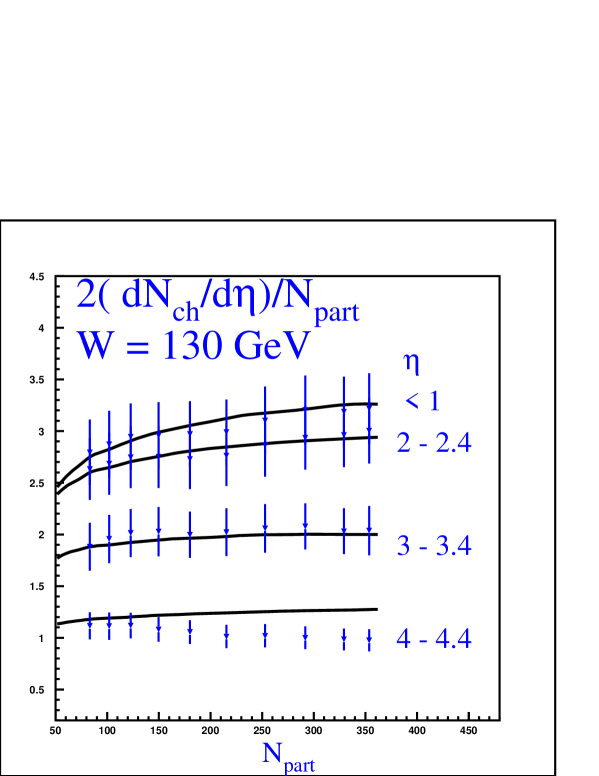
Figure 17: Centrality dependence of charged hadron production per participant at different pseudo-rapidity $\eta$ intervals in $Au-Au$ collisions at $\sqrt{s}=130$ GeV; from Kharzeev and Levin (2001), the data are from PHOBOS Coll. (2000).

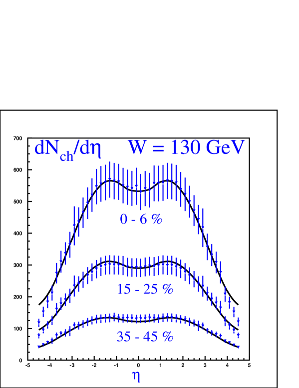
Figure 18: Pseudo–rapidity dependence of charged hadron production at different cuts on centrality in $Au-Au$ collisions at $\sqrt{s}=130$ GeV; from Kharzeev and Levin (2001), the data are from PHOBOS Coll. (2000).

The results for the $Au-Au$ collisions at $\sqrt{s}=130$ GeV are presented in Figs 17 and 18. In the calculation, we use the results on the dependence of saturation scale on the mean number of participants at $\sqrt{s}=130$ GeV from Kharzeev and Nardi (2001), see Table 2 of that paper. The mean number of participants in a given centrality cut is taken from the PHOBOS paper PHOBOS Coll. (2000). One can see that both the centrality dependence and the rapidity dependence of the $\sqrt{s}=130$ GeV PHOBOS data are well reproduced below $\eta\simeq\pm 4$. The rapidity dependence has been evaluated with $\lambda=0.25$, which is within the range $\lambda=0.25\div 0.3$ inferred from the HERA data Golec-Biernat and Wüsthoff (1999). The discrepancy above $\eta\simeq\pm 4$ is not surprising since our approach does not properly take into account multi–parton correlations which are important in the fragmentation region.

Our predictions for $Au-Au$ collisions at $\sqrt{s}=200$ GeV are presented in Kharzeev and Levin (2001). The only parameter which governs the energy dependence is the exponent $\lambda$, which we assume to be $\lambda\simeq 0.25$ as inferred from the HERA data. The absolute prediction for the multiplicity, as explained above, bears some uncertainty, but there is a definite feature of our scenario which is distinct from other approaches. It is the dependence of multiplicity on centrality, which around $\eta=0$ is determined solely by the running of the QCD strong coupling Kharzeev and Nardi (2001). As a result, the centrality dependence at $\sqrt{s}=200$ GeV is somewhat less steep than at $\sqrt{s}=130$. While the difference in the shape at these two energies is quite small, in the perturbative mini-jet picture this slope should increase, reflecting the growth of the mini-jet cross section with energy Wang and Gyulassy (2001).

3.2.5 Further tests

Checking the predictions of the semi–classical approach for the centrality and pseudo–rapidity dependence at $\sqrt{s}=200$ GeV is clearly very important. What other tests of this picture can one devise? The main feature of the classical emission is that it is coherent up to the transverse momenta of about $\sqrt{2}\ Q_{s}$ (about $\simeq 2$ GeV/c for central $Au-Au$ collisions). This means that if we look at the centrality dependence of particle multiplicities above a certain value of the transverse momentum, say, above $1$ GeV/c, it should be very similar to the dependence without the transverse momentum cut-off. On the other hand, in the two–component “soft plus hard” model the cut on the transverse momentum would strongly enhance the contribution of hard mini–jet production processes, since soft production mechanisms presumably do not contribute to particle production at high transverse momenta. Of course, at sufficiently large value of the cutoff all of the observed particles will originate from genuine hard processes, and the centrality dependence will become steeper, reflecting the scaling with the number of collisions. It will be very interesting to explore the transition to this hard scattering regime experimentally.

Another test, already discussed above (see Eq. (100)) is the study of azimuthal correlations between the produced high $p_{t}$ particles. In the saturation scenario these correlations should be very small below $p_{t}\simeq 2$ GeV/c in central collisions. At higher transverse momenta, and/or for more peripheral collisions (where the saturation scale is smaller) these correlations should be much stronger.

3.3 Does the vacuum melt?

The approach described above allows us to estimate the initial energy density of partons achieved at RHIC. Indeed, in this approach the formation time of partons is $\tau_{0}\simeq 1/Q_{s}$, and the transverse momenta of partons are about $k_{t}\simeq Q_{s}$. We thus can use the Bjorken formula and the set of parameters deduced above to estimate Kharzeev and Nardi (2001)

$$\epsilon\simeq{<k_{t}>\over\tau_{0}}\ {d^{2}N\over d^{2}bd\eta}\simeq Q_{s}^{2}\ {d^{2}N\over d^{2}bd\eta}\simeq 18\ {\rm{GeV/fm^{3}}}$$ (124)

for central $Au-Au$ collisions at $\sqrt{s}=130$ GeV. This value is well above the energy density needed to induce the QCD phase transition according to the lattice calculations. However, the picture of gluon production considered above seems to imply that the gluons simply flow from the initial state of the incident nuclei to the final state, where they fragment into hadrons, with nothing spectacular happening on the way. In fact, one may even wonder if the presence of these gluons modifies at all the structure of the physical QCD vacuum.

To answer this question theoretically, we have to possess some knowledge about the non–perturbative vacuum properties. While in general the problem of vacuum structure still has not been solved (and this is one of the main reasons for the heavy ion research!), we do know one class of vacuum solutions – the instantons. It is thus interesting to investigate what happens to the QCD vacuum in the presence of strong external classical fields using the example of instantons Kharzeev, Kovchegov and Levin (2002).

Figure 19: Distributions of instanton sizes in vacuum for QCD with three light flavors (upper curve) versus the distribution of instanton sizes in the saturation environment produced by a collision of two identical nuclei for $c=1$ (middle curve) and $c=2\ln 2$ (lower curve) with $Q_{s}^{2}\,=\,2\,\mbox{GeV}^{2}$; from Kharzeev, Kovchegov and Levin (2001).

The problem of small instantons in a slowly varying background field was first addressed in Callan, Dashen and Gross (1979); Shifman, Vainshtein and Zakharov (1980) by introducing the effective instanton Lagrangian $L^{I(\overline{I})}_{eff}(x)$

$$L_{eff}^{I}(x_{0})\,=\,\int d\rho\,n_{0}(\rho)\,dR\,\exp\left(-\frac{2\pi^{2}}{g^{2}}\,\rho^{2}\,\overline{\eta}^{M}_{a\mu\nu}\,R^{aa^{\prime}}\,G^{a^{\prime}}_{\mu\nu}(x_{0})\right)$$ (125)

in which $n_{0}(\rho)$ is the instanton size distribution function in the vacuum, $\overline{\eta}^{M}_{a\mu\nu}$ is the ’t Hooft symbol in Minkowski space, and $R^{aa^{\prime}}$ is the matrix of rotations in color space, with $dR$ denoting the averaging over the instanton color orientations.

The complete field of a single instanton solution could be reconstructed by perturbatively resumming the powers of the effective instanton Lagrangian which corresponds to perturbation theory in powers of the instanton size parameter $\rho^{2}$. In our case here the background field arises due to the strong source current $J_{\mu}^{a}$. The current can be due to a single nucleus, or resulting from the two colliding nuclei. Perturbative resummation of powers of the source current term translates itself into resummation of the powers of the classical field parameter $\alpha_{s}^{2}A^{1/3}$ McLerran and Venugopalan (1994); Kovchegov (1996). Thus the problem of instantons in the background classical gluon field is described by the effective action in Minkowski space

$$S_{eff}\,=\,\int d^{4}x\left(-\frac{1}{4g^{2}}G^{a}_{\mu\nu}(x)G^{a}_{\mu\nu}(x)\,+\,L^{I}_{eff}(x)\,+\,L^{\overline{I}}_{eff}(x)\,+\,J_{\mu}^{a}\,A_{\mu}^{a}(x)\right).$$ (126)

The problem thus is clearly formulated; by using an explicit form for the radiated classical gluon field, it was possible to demonstrate Kharzeev, Kovchegov and Levin (2002) that the distribution of instantons gets modified from the original vacuum one $n_{0}(\rho)$ to

$$n_{sat}^{AA}(\rho)\,=\,n_{0}(\rho)\,\exp\left(-\frac{c\,\rho^{4}Q_{s}^{4}}{8\,\alpha_{s}^{2}\,N_{c}\,(Q_{s}\tau_{0})^{2}}\right),$$ (127)

where $\tau_{0}$ is the proper time. The result Eq. (127) shows that large size instantons are suppressed by the strong classical fields generated in the nuclear collision (see Fig. 19). The vacuum does melt!

References

- (1) Field, R.D., Applications of Perturbative QCD, Addison-Wesley, New York, USA, 1989.
- (2) Altarelli, G. in this volume.
- (3) Ellis, R.K., Stirling, W.J. and Webber B.R., QCD and Collider Physics, Cambridge University Press, Cambridge, UK, 1996.
- (4) Muta, T., Foundations of Quantum Chromodynamics, World Scientific, Singapore, Singapore, 1987.
- (5) Landau, L.D. and Pomeranchuk, I.Y., Dokl. Akad. Nauk Ser. Fiz. 102:489, 1955; also published in The Collected Papers of L.D. Landau. Edited by D. Ter Haar, Pergamon Press, 1965. pp. 654-658.
- (6) Gribov, V.N., Eur. Phys. J. C 10:71, 1999 [arXiv:hep-ph/9807224];
-
(7)
Gross, D.J. and Wilczek, F.,
Phys. Rev. Lett. 30:1343, 1973;
Politzer, H.D., Phys. Rev. Lett. 30:1346, 1973. - (8) Nielsen, N.K., Am. J. Phys. 49:1171, 1981.
- (9) Landau, L.D. and Lifshits, E.M., Quantum Mechanics: Nonrelativistic Theory, Landau-Lifshits physics course vol. 3, Pergamon Press, Oxford, UK, 1965.
- (10) Bethke, S., J. Phys. G 26:R27, 2000 [arXiv:hep-ex/0004021].
- (11) Wilson, K., Phys.Rev. D10:2445, 1974.
-
(12)
Adler, S.L.,
Phys. Rev. 177:2426, 1969;
Bell, J.S. and Jackiw, R., Nuovo Cim. A60:47, 1969. - (13) Schäfer, T. and Shuryak, E.V. Rev. Mod. Phys. 70:323, 1998 [arXiv:hep-ph/9610451].
- (14) Forkel, H., arXiv:hep-ph/0009136.
-
(15)
Peccei, R.D. and Quinn, H.R.,
Phys. Rev. Lett. 38:1440, 1977;
Phys. Rev. D16:1791, 1977;
Wilczek, F., Phys. Rev. Lett. 40:279, 1978;
Weinberg, S., Phys. Rev. Lett. 40:223, 1978. - (16) Lee T.D. and Wick, G.C., Phys. Rev. D9:2291, 1974.
-
(17)
Kharzeev, D.E., Pisarski R.D. and Tytgat, M.H.,
Phys. Rev. Lett. 81:512, 1998
[arXiv:hep-ph/9804221];
Kharzeev, D.E. and Pisarski, R.D., Phys. Rev. D61:111901, 2000 [arXiv:hep-ph/9906401]. - (18) Glauber, R.J., “High Energy Collision theory” in Lectures in Theoretical Physics, vol. 1, W. E. Brittin and L. G. Duham (eds.) Interscience, New York, 1959.
- (19) Gribov, V.N., Sov. Phys. JETP 29:483, 1969 [Zh. Eksp. Teor. Fiz. 56:892, 1969)].
- (20) Gribov, V.N., arXiv:hep-ph/0006158.
- (21) Abramovsky, V.A., Gribov V.N. and Kancheli, O.V., Yad. Fiz. 18:595, 1973 [Sov. J. Nucl. Phys. 18:308, 1973].
- (22) Low, F.E., Phys. Rev. D12:163, 1975; Nussinov, S., Phys. Rev. Lett. 34:1286, 1975.
-
(23)
Froissart, M.,
Phys. Rev. 123:1053, 1961;
Martin, A., Phys. Rev. 129:1432, 1963. - (24) Schwimmer, A., Nucl. Phys. B94:445, 1975.
-
(25)
Gribov, V.N.,
Sov. Phys. JETP 26:414, 1968
[Zh. Eksp. Teor. Fiz. 53:654, 1968];
Abarbanel, H.D., Bronzan, J.B., Sugar R.L. and White A.R., Phys. Rept. 21:119, 1975. - (26) Kharzeev, D.E., Nucl. Phys. A699:95, 2002 [arXiv:nucl-th/0107033].
- Gribov, Levin and Ryskin (1983) Gribov, L.V., Levin, E.M. and Ryskin, M.G., Phys. Rept. 100:1, 1983.
- Mueller and Qiu (1986) Mueller, A.H. and Qiu, J.-W., Nucl. Phys. B268:427, 1986.
- Blaizot and Mueller (1987) Blaizot, J.P. and Mueller, A.H., Nucl. Phys. B289:847, 1987.
- McLerran and Venugopalan (1994) McLerran, L.D. and Venugopalan, R., Phys. Rev. D49:2233, 1994; D49:3352, 1994.
- Iancu, Leonidov, McLerran (2002) Iancu, I., Leonidov, A., and McLerran, L. hep-ph/0202270.
- Mueller (2001) Mueller, A.H., hep-ph/0111244.
- Kharzeev, Kovchegov and Levin (2001) Kharzeev, D., Kovchegov, Yu. and Levin, E., Nucl. Phys. A690:621, 2001;
- Nowak, Shuryak and Zahed (2001) Nowak, M., Shuryak, E., and Zahed, I., Phys.Rev. D64:034008, 2001.
- Kharzeev, Kovchegov and Levin (2002) Kharzeev, D., Kovchegov, Yu. and Levin, E., Nucl.Phys.A699:745, 2002.
- Berestetskii,Lifshitz and Pitaevskii (1982) Berestetskii, V. B., Lifshitz, E.M. and Pitaevskii, L.P., “Quantum electrodynamics”, Oxford New York, Pergamon Press, 1982.
- Kharzeev and Nardi (2001) Kharzeev, D. and Nardi, Phys. Lett. B507:121, 2001.
- Kharzeev, Lourenço, Nardi and Satz (1997) Kharzeev, D., Lourenço, C., Nardi, M. and Satz, H., Z.Phys. C74:307, 1997.
- De Jager, De Vries and De Vries (1974) De Jager, C., De Vries, H. and De Vries, C., Atom. Nucl. Data Tabl. 14:479, 1974.
- Kharzeev and Levin (2000) Kharzeev, D. and Levin, E., Nucl. Phys. B578:351, 2000.
- Gyulassy and McLerran (1997) Gyulassy, M. and McLerran, L., Phys. Rev. C56:2219, 1997.
- Wang and Gyulassy (2001) Wang, X.N. and Gyulassy, M., Phys. Rev. Lett. 86:3496, 2001.
- Dokshitzer (1998) Dokshitzer, Yu.L., hep-ph/9812252.
- PHENIX Coll. (2001) Adcox, K. et al., (The PHENIX Collaboration), Phys. Rev. Lett. 86:3500, 2001; Phys. Rev. Lett. 87:052301, 2001; Milov, A. et al., (The PHENIX Collaboration), nucl-ex/0107006.
- STAR Coll. (2001) Adler, C. et al., (The STAR Collaboration), Phys. Rev. Lett. 87:112303, 2001; Phys. Rev. Lett. 87:082301, 2001.
- PHOBOS Coll. (2000) Back, B. et al., PHOBOS Coll., Phys. Rev. Lett. 85:3100, 2000; Phys. Rev. Lett. 87:102303, 2001; nucl-ex/0105011; nucl-ex/0108009.
- BRAHMS Coll. (2001) Bearden I.G. et al., (The BRAHMS Collaboration), Phys. Rev. Lett. 87:112305, 2001; nucl-ex/0102011; nucl-ex/0108016
- Golec-Biernat and Wüsthoff (1999) Golec-Biernat, K. and Wüsthoff, M., Phys. Rev. D59:014017, 1999; Phys. Rev. D60:114023, 1999; Stasto, A., Golec-Biernat, K. and Kwiecinski, J., Phys. Rev. Lett. 86:596, 2001.
- Kharzeev and Levin (2001) Kharzeev, D. and Levin, E., Phys. Lett. B523:79, 2001.
-
Eskola, Kajantie, Ruuskanen and Tuominen (2000)
Eskola, K.J., Kajantie, K. and Tuominen, K., Phys. Lett. B497:39, 2001;
Eskola, K.J., Kajantie, K., Ruuskanen, P.V. and Tuominen, K., Nucl. Phys. B 570:379, 2000. - Callan, Dashen and Gross (1979) Callan, C.G., Dashen, R. and Gross, D.J., Phys. Rev. D19:1826, 1979.
- Shifman, Vainshtein and Zakharov (1980) Shifman, M.A., Vainshtein, A.I., Zakharov, V.I., Nucl. Phys. B165:45, 1980.
- Kovchegov (1996) Kovchegov, Yu.V., Phys. Rev. D54:5463, 1996); 55:5445, 1997.