Approximate Solutions of Quantum Equations

for Electron Gas in Plasma

M.Dvornikov

Department of Theoretical Physics, Moscow State University

119992 Moscow, Russia

S.Dvornikov

Acoustical Institute, ’Shvernika’ street, 4,

117036 Moscow, Russia

G.Smirnov

Kamchatka Hydrophysical Institute,

KHPI, Kamchatka region, Viliutchinsk, Russia

Abstract

We have obtained the solutions of linearized Shrödinger equation for spherically and axially symmetrical electrons density oscillations in plasma in the approximation of the self-consistent field. It was shown that in the center or on the axis of symmetry of such a system the static density of electrons can enhance, which leads to the increasing of density and pressure of ion gas. We suggest that this mechanism could be realized in nature as rare phenomenon called the ’fireball’ and could be used in carrying out the research concerning controlled fusion.

If a volume charge appears in electroneutral plasma, i.e. electrons density increases or decreases in some finite area, then, after an external influence is over, the oscillating process consisting in periodical changes of the sign of the considered volume charge is known to appear. It is necessary to remind that the frequency of this process $\omega_{p}$ called plasma frequency is related to free electrons density in the plasma $n_{0}$ by the formula

$$\omega_{p}^{2}=\frac{{4\pi e^{2}n_{0}}}{{m}},$$ (1)

where $e$ and $m$ are the charge and the mass of the electron.

We will assume electrons in plasma to be a quantum many body system. Such an assumption is due to the fact that, as it will be shown below, the solutions obtained have characteristic sizes of atomic order. It is known that the classical dynamics of $N$ interacting particles can be represented by the system of differential equations of motion in configuration space of $3N$-dimensions, or in $6N$-dimensional phase space, as well as by the system of partial differential equations in three-dimensional physical space and as the dynamics of singular material fields (see Refs. [1, 2, 3]). The transfer to the quantum-mechanical description is realized by changing the dynamic functions to Hermitian operators. In this case the dimensionality of the configuration space is conserved and the state of the system is completely defined by the wave functions in the $3N$-dimensional space.

Shrödinger equation as it was shown in Refs. [3, 4], could be presented in the form of the system of equations in physical space and having the same form as the equations of hydrodynamics. In these works the quantum-mechanical system of $N$ particles with arbitrary masses and charges, interacting between itself by Coulomb forces and with external classical electromagnetic field characterized by vector $\vec{A}$ and scalar $\varphi$ potentials has been considered.

In this approach the complex $\Psi$ function introduced in three-dimensional space has the following form

$$\Psi\left({{\vec{r}},t}\right)=\sqrt{n_{e}\left({{\vec{r}},t}\right)}e^{\frac{{i}}{{\hbar}}\sigma\left({\vec{r}},t\right)},$$ (2)

where $\left|\Psi\right|^{2}=n_{e}({\vec{r}},t)$ is the density of electrons and $\Psi$ function satisfies the partial differential equation:

$$i\hbar\frac{{\partial\Psi}}{{\partial t}}={\hat{H}}\Psi.$$ (3)

The Hamiltonian in Eq. (3) is expressed in the following way

$${\hat{H}}=\frac{{1}}{{2m}}\left({\frac{{\hbar}}{{i}}{\vec{\nabla}}-\frac{{e}}{{c}}{\vec{A}}\left({\vec{r}},t\right)}\right)^{2}+e\varphi+e^{2}\int\limits_{{\vec{r}}_{0}}^{\vec{r}}{d^{3}{\bf r}^{\prime}G\left({\vec{r}}-{\vec{r}}^{\prime}\right)\left|{\Psi}\right|^{2}+\theta\left({\vec{r}},t\right)},$$ (4)

where $G\left({\vec{r}}-{\vec{r}}^{\prime}\right)={\frac{1}{\left|{\vec{r}}-{\vec{r}}^{\prime}\right|}}$.

In the Eq. (4) the first two terms are the components of one electron Hamiltonian in the external electromagnetic field, the third term represents the potential energy of the electron in the self-consistent electrostatic field created by the whole electron system, with density of number of particles being equal to $\left|\Psi\right|^{2}$. The function $\theta\left({\vec{r}},t\right)$ describing exchange interactions between electrons has the following form

$$\theta\left({\vec{r}},t\right)=\frac{{\hbar^{2}}}{{2m}}\frac{{\Delta\Psi}}{{\left|{\Psi}\right|}}+\int\limits_{{\vec{r}}_{0}}^{\vec{r}}{\frac{{dp_{e}\left({\vec{r}},t\right)}}{{\left|{\Psi}\right|^{2}}}}+e^{2}\int{d^{3}{\bf r}^{\prime}\int\limits_{{\vec{r}}_{0}}^{\vec{r}}{d}G\left({{\vec{r}}-{\vec{r}}^{\prime}}\right)\frac{{q_{2}\left({{\vec{r}},{\vec{r}}^{\prime},t}\right)}}{{\left|{\Psi}\right|^{2}}}},$$ (5)

where $p_{e}\left({\vec{r}},t\right)$ is the pressure of electron gas, $q_{2}\left({\vec{r}},{\vec{r}}^{\prime},t\right)$ is the correlation function.

Therefore, in order to resolve exactly the considered problem one should take into account all terms in the Eq. (5). However, we will assume that the contribution of exchange interactions to the dynamics of free electrons in plasma is much smaller than that of the potential of self-consistent electrostatic field. Then, in describing the dynamics of electron gas we will neglect the function $\theta\left({\vec{r}},t\right)$. As it will be seen from further speculations, this rough approximation allows us to get some consequences which are close to those obtained from the consideration of the similar problem within the classical approach.

Let us consider the neutral plasma, formed by the singly ionized gas, with the energy of electrons being more than the potential of ionization of this gas. We will suppose that this plasma possesses a spherical symmetry for density and velocities distribution of the electron and the ion gases. Taking into account the small mobility of heavy ions in gas compared to that of electrons we will suppose that the density of ions is the constant value $n_{i}\left({\vec{r}},t\right)=n_{0}$. We will also consider that in our case there are no external electromagnetic fields except those of positively charged ions. It is worth mentioning that the magnetic field in the system is equal to zero. The potential of self-consistent field created by the density of electron gas is represented by the formula (using spherical coordinates):

$$U_{e}=e\int\limits_{{\vec{r}}_{0}}^{\vec{r}}d^{3}{\bf r}G({\vec{r}}^{\prime}-{\vec{r}}){{\left|{\Psi}\right|^{2}}}=4{\pi}e\int\limits_{r}^{\infty}{\frac{dR}{R^{2}}}\int\limits_{0}^{R}x^{2}{{\left|{\Psi}(x,t)\right|^{2}}}dx.$$ (6)

Similarly, for the potential $\varphi$ of singly ionized gas with density of ions $n_{i}(r,t)$ one has

$$\varphi=-4{\pi}e\int\limits_{r}^{\infty}{\frac{dR}{R^{2}}}\int\limits_{0}^{R}x^{2}n_{i}(x,t)dx.$$ (7)

Thus, taking into account Eq. (6) and Eq. (7), the Eq. (3) can be represented in the following way

$$i\hbar\frac{{\partial\Psi}}{{\partial t}}+\frac{{\hbar^{2}}}{{2m}}\Delta\Psi-4\pi e^{2}\Psi F({{\left|{\Psi}\right|^{2}}}-n_{0})=0,$$ (8)

where $\Delta={\frac{\partial^{2}}{\partial r^{2}}}+{\frac{2}{r}}{\frac{\partial}{\partial r}}$ is the Laplas operator in the spherical coordinate system, $F(\ldots)=\int\limits_{r}^{\infty}{\frac{dR}{R^{2}}}\int\limits_{0}^{R}x^{2}(\ldots)dx.$

Moreover, we demand the system to be electroneutral as a whole, i.e. the condition must be satisfied:

$$\lim_{R\rightarrow\infty}{\frac{1}{R^{3}}}\int\limits_{0}^{R}x^{2}{{\left|{\Psi}(x,t)\right|^{2}}}dx={\frac{n_{0}}{3}}.$$ (9)

We will search for a solution of the Eq. (8) in the form:

$$\Psi=\Psi_{0}+\chi e^{-i\omega t}\quad.$$ (10)

Supposing that $\left|\Psi_{0}\right|^{2}=n_{0}$ and $\left|\chi\right|\ll\left|\Psi_{o}\right|$, we get $\left|\Psi_{0}\right|^{2}=n_{0}+\Psi_{0}f+\left|\chi\right|^{2}$, where $f=\chi e^{-i\omega t}+\chi^{*}e^{i\omega t}$. Taking into account that ${\left|\chi\right|}\ll\left|\Psi_{o}\right|$, we obtain $\left|\Psi_{0}\right|^{2}\approx n_{0}+\Psi_{0}f$.

Then, we substitute Eq. (10) and approximate expression for $\left|\Psi_{0}\right|^{2}$ in Eq. (8). Having considered the complex-conjugate equation together with the obtained one, it was easy to get:

$$\hbar\omega f+\frac{{\hbar^{2}}}{{2m}}\Delta f-4\pi e^{2}\Psi_{0}\left({2\Psi_{0}+f}\right)F\left({f}\right)=0.$$ (11)

For the total linearization, it is necessary to suppose that $2\Psi_{0}+f\cong 2\Psi_{0}$ in the third term of the equation involved. Then, we represent the function $\chi$ through its real and imaginary parts: $\chi=\chi_{1}+i\chi_{2}$. Hence $f=\chi_{1}\cos\omega t+\chi_{2}\sin\omega t$, and Eq. (8) can be divided into two independent similar equations for $\chi_{1}$ and $\chi_{2}$:

$$\hbar\omega\chi_{n}+\frac{{\hbar^{2}}}{{2m}}\Delta\chi_{n}-8\pi e^{2}n_{0}F\left({\chi_{n}}\right)=0,\quad n=1,2.$$ (12)

One can find out the functions $\chi_{n}=B_{n}\frac{{sin\gamma r}}{{r}}$ are the solutions of of the Eq. (12) if $\gamma$ satisfies the following dispersion relation

$$\gamma^{2}={\frac{\omega m}{\hbar}}\left[1\pm\left(1-4{\frac{\omega_{p}^{2}}{\omega^{2}}}\right)^{1/2}\right],$$ (13)

where $\omega_{p}$ is determined in Eq. (1). The positive part of the dependence of $\gamma$ on the frequency $\omega$ is presented in the Fig. 1. It is worth noticing that if the values of $B_{n}$ are limited, the expressions for $\chi_{n}$ satisfies the condition of system electroneutrality (9).

From the expression (13) one can see that the frequency $\omega=2\omega_{p}$ is the critical value, since for frequencies less than $2\omega_{p}$, $\gamma$ becomes a complex value and under these circumstances the oscillations of the electron gas are absent. It is necessary to remind that in using the classical approach to the similar problem one gets the value $\omega=\omega_{p}$ for the critical frequency.

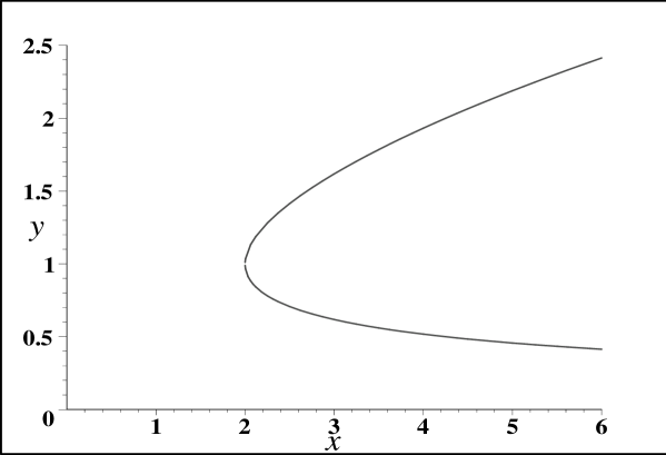
Figure 1: The coeficient $y=\gamma\left(2\omega_{p}{\frac{\hbar}{m}}\right)^{-1/2}$ versus the parameter $x={\frac{\omega}{\omega_{p}}}$. If $\omega=2\omega_{p}$, then $\gamma_{1,2}=\pm\left({\frac{2m\omega_{p}}{\hbar}}\right)^{1/2}$. If $\omega\gg 2\omega_{p}$, for the upper branch we have $\gamma_{1,2}=\pm\left({\frac{2m\omega}{\hbar}}\right)^{1/2}$, and for the lower branch $\gamma_{3,4}=\pm\left({\frac{2m\omega_{p}^{2}}{\omega\hbar}}\right)^{1/2}$.

For example, for the density $n_{0}=2.7\cdot 10^{19}cm^{-3}$, i.e. for completely singly ionized gas under the atmospheric pressure and when $\omega=2\omega_{p}$, the frequency of electron oscillations is:

$$\nu={\frac{\omega_{p}}{\pi}}=2\left({\frac{e^{2}n_{0}}{\pi m}}\right)^{1/2}\approx 9\cdot 10^{13}Hz.$$

This frequency corresponds to the electromagnetic radiation in the infrared range with the wavelength $\lambda={\frac{c}{\nu}}\approx 3\cdot 10^{-4}cm$. In this case $\gamma_{1,2}=\pm\left({\frac{2m\omega_{p}}{\hbar}}\right)^{1/2}\approx\pm 2.3\cdot 10^{7}cm^{-1}$, the size of central region $\delta$, where the most intensive oscillations of the electron gas are observed, is equal to $\pi/\gamma\approx 1.4\cdot 10^{-7}cm$.

It is necessary to remind that the exact expression for the density of electron gas in searching for the solution in the form of the Eq. (10) is presented as $\left|\Psi_{0}\right|^{2}=n_{0}+\Psi_{0}f+\left|\chi\right|^{2}$. Let us define in this expression $\Psi_{0}f$ and ${\bar{n}}_{e}=\left|\chi\right|^{2}+n_{0}$ as the dynamic and static components of density respectively. In deriving the approximate linearized equation (12) the function $\left|\chi\right|^{2}$ was supposed to be small and thus neglected. This procedure is not correct because the integral $F\left({\left|\chi\right|^{2}}\right)$ for the function $\chi=B\frac{{sin\gamma r}}{{r}}$ is divergent. However, we assumed that the density of ion gas was constant throughout the volume because of the small mobility of heavy ions. This assumption is valid for the frequently oscillating dynamic component, but $\left|\chi\right|^{2}$ does not depend on time. Therefore, it is naturally to expect that under some conditions the negative volume charge, described by this function, will be compensated (or neutralized) by removing positive ions, that will result in local changing of density and pressure of the ion gas.

Indeed, it can be shown that for our case the condition of static stability of the ion gas is (see, for instance, Refs. [5, 6]):

$$kT{\frac{\partial n_{i}}{\partial r}}={\frac{4\pi e^{2}}{r^{2}}}n_{i}\int\limits_{0}^{r}\left(n_{i}-{\bar{n}}_{e}\right)x^{2}dx$$ (14)

where $k$ is Boltsman constant, $T$ is the ion gas temperature, $n_{i}$ is the ions density, ${\bar{n}}_{e}$ is the static electrons density.

We demand that the ions density is equal to static electrons density with high level of accuracy $n_{i}\approx{\bar{n}}_{e}=n_{0}+B^{2}{\frac{\sin^{2}\gamma r}{r^{2}}}$. Then, from Eq. (14) we get the following inequality: ${\frac{kT}{4\pi e^{2}}}{\frac{r^{2}}{n_{i}}}\left|{\frac{\partial n_{i}}{\partial r}}\right|\ll 1$. Having substituted the expression for $n_{i}$ in the last formula, we obtained the condition of the neutralization: ${\frac{kTB^{2}\gamma}{4\pi e^{2}n_{0}}}\ll 1$. Taking into account that ions density in the center of the system should be equal to $n_{c}=B^{2}\gamma^{2}$, this condition can be rewritten in the following way:

$$n_{c}\ll{\frac{4\pi e^{2}\gamma}{kT}}n_{0}.$$ (15)

For instance, for $T=1000^{0}K$ and the value $\gamma=2.3\cdot 10^{7}cm^{-1}$ which was obtained above we get $n_{c}\ll 500n_{0}$. In deriving the solution of our problem we assumed that $n_{c}\ll n_{0}$. Thus, we can conclude that, if the condition (15) is satisfied, the ion charge is undoubtedly compensated by the supplementary static electron charge and the divergence in the integral $F(|\Psi|^{2}-n_{i})$ can be eliminated.

Hence, the approximate, linearized theory trends to describe the pressure enhancement of the ion gas in the center of symmetrically oscillating electron gas.

It is worth mentioning that along with spherically symmetrical solution of the Eq. (12), there is at least one axially-symmetrical one which has the form:

$$\Psi=n_{0}^{1/2}+BJ_{0}(\gamma r)e^{-i\omega t},$$

where $J_{0}$ is the zero-order Bessel function. In this case the dispersion relation takes the same form as Eq. (13). All consequences obtained for spherically-symmetrical oscillations are valid and for this case too.

While considering nonlinear Shrödinger equation (8), it can be seen that along with the components of frequency $\omega$, the terms which do not depend on time as well as on frequencies $2\omega$, $3\omega$ and etc. appear. One can make sure of this representing the solution of the Eq. (8) in the form: $\Psi(r,t)=\Psi_{0}+\sum\limits_{k=1}^{\infty}\Psi_{k}(r,t),$ where $\Psi_{1}=B_{1}e^{-i\omega t}{\frac{\sin\gamma r}{r}}$.

In Ref. [7] we put forward the hypothesis that in this case the static density of electron gas could attain great values. Density and pressure of ion gas are also great in the center of such systems. Thus, along with the heating of the central area resulted from intensive movement of electrons, there will be a possible running of nuclear fusion reactions of corresponding nuclei in gas.

This process seems to support the existence of the enigmatic natural phenomena, known as ’fireball’. If vapors of water which are present in atmosphere contain deuterium in the amount of $\approx 1/5000$ under normal conditions, the running the nuclear fusion reactions will release the energy, which support the oscillations of electron gas and prevent the recombination of plasma. Taking into account small sizes of the central (active) regions and small amount of deuterium in atmosphere, it is possible to use the term ’microdose’ thermonuclear reaction for process in question. Axially-symmetrical oscillation of the electron gas is likely to appear as very seldom observed type of a ’fireball’ in the form of shining, sometimes closed cord [8]. Uncomplicated calculation shows that energy released in deuterium nuclei fusion in $1dm^{3}$ of vapors of water (the average size of a ’fireball’) has the value of about $1MJ$, that corresponds to evaluations of energy released by some observed ’fireballs’ (see, for example, Refs. [8, 9]).

Groups and separate researchers developing the problem of the controlled fusion are suggested to pay attention to self-consistent, radially and axially oscillating electron plasmoids as a base models to self-supported thermonuclear reactions. The authors of the present article have certain experience in generating ball-like plasma structures which proves the correctness of the chosen model.

References

- [1] L. Landau and E. Lifshitz, The Classical Theory of Fields Nauka, Moscow, (1988).
- [2] L. Landau and E. Lifshitz, Quantum Mechanics - Non-relativistic Theory Nauka, Moscow, (1989).
- [3] M. Drofa and L. Kuzmenkov, Theor.Math.Phys. 108, 849, (1996); Teor.Mat.Fiz. 108, 3, (1996).
- [4] L. Kuzmenkov and S. Maksimov, Theor.Math.Phys. 118, 227, (1999); Teor.Mat.Fiz. 118, 287, (1999).
- [5] N. Bogoliubov (jr.) and B. Sadovnikov, Some Problems of Statistical Mechanics Visshaya Shkola, Moscow, (1975) (in Russian).
- [6] E. Lifshitz and L. Pitaevskii, Physical Kinetics Nauka, Moscow, (1979).
- [7] M. Dvornikov, S. Dvornikov and G. Smirnov, Appl.Math.&Eng.Phys. 1, 9, (2001) (in Russian).
- [8] I. Stakhanov, Physical Nature of the Fireball Energoatomizdat., Moscow, (1985) (in Russian).
- [9] J. Frenkel, Zh.Eksp.Teor.Phys. 10, 1424, (1940).