Exponential Basis in Two-Sided Variational Estimates of Energy for Three-Body Systems

Abstract

By the use of the variational method with exponential trial functions the upper and lower bounds of energy are calculated for a number of non-relativistic three-body Coulomb and nuclear systems. The formulas for calculation of upper and lower bounds for exponential basis are given, the lower bounds for great part of systems were calculated for the first time. By comparison of calculations for different bases the efficiency of exponential trial functions and their universality in respect to masses of particles and interaction are demonstrated. The advantage of exponential basis manifests mostly evident for the systems with comparable masses, though its use in one-center and two-center problems is justified too. For effective solution of two-center problem a carcass modification of the trial function is proposed. The stability of various three-particle Coulomb systems is analyzed.

1 Introduction

Among existing methods of calculation of non-relativistic bounded systems the variational method seems to be the most universal one as it is applied equally well for the solution of atomic and nuclear problems. It is essential that the variational method allows to find not only the upper ($E_{U}$) but also the lower ($E_{L}$) estimates of the energy. As to potentiality of the method, there are many examples of highly accurate calculations of three- and more-particle systems [1]-[21]. For instance in the three-body Coulomb problem the precision is amounted up to a score of decimal places. Of course in real physical systems the relativistic and other effects lead to corrections in the energy already in 5–7-th decimal place and therefore, in practical use a variational procedure which ensures a reasonable accuracy with least computational efforts may be acceptable.

Historically the first variational expansion in a three-particle problem was suggested by Hylleraas in perimetrical coordinates in the form of exponent function multiplied by a polynomial with integer nonnegative powers. Later negative and fractional powers were added [1], [2], besides Frankowski and Pekeris [3] introduced logarithmic terms. In the next this basis is referred as ’polynomial’ one.

Another possibility is to use a purely exponential basis. It ensures a good flexibility of the variational expansion due to the presence of many scale nonlinear parameters. Whereas the Hylleraas basis is practically oriented on solution of uni-center Coulomb problems the exponential basis is good for systems with any masses of particles and types of their interaction [4]. Besides, the calculations with exponential basis are more simple and uniform whereas for polynomial basis they became more and more complicated as number of terms increases, especially if the logarithmic terms are included.

Instead of exponents another non-polynomial functions, gaussians, can be used. They are not less than exponents fitted for the systems with any masses of particles, moreover they are applicable to systems with arbitrary number of particles. For this basis all the formulas needed for calculation of both the upper and lower bounds are given in paper [5], and different 3-, 4-, and 5-particle systems were calculated there. For the upper bound a generalization is given in article [6] for arbitrary orbital moments. Nevertheless, our analysis have shown that at least for three-body variational calculations with not very high number of parameters the precision for gaussian basis is lower than for exponential one.

Our principal goal was not the striving for improvement of existing super-high precision calculations but the analysis of efficiency of exponential and partly gaussian trial functions for evaluation of the upper and lower variational bounds. For this purpose the Coulomb and nuclear systems of particles with different masses and types of interaction are considered and the results of calculations are compared with those published in literature.

To facilitate such a comparison we will characterize the accuracy of calculations of $E_{U}$ and $E_{L}$ by the values:

$$\delta_{U}=-\lg\left(\frac{E_{0}-E_{U}}{E_{0}}\right),\qquad\delta_{L}=-\lg\left(\frac{E_{L}-E_{0}}{E_{0}}\right),$$ (1)

which determine the number of correct decimal places of $E_{U}$ and $E_{L}$ respectively, $E_{0}$ being the exact value of the energy.

The universality of exponential basis in respect to masses of particles allows us to analyze the problem of stability of different Coulomb three-particle systems.

2 Method of calculation

In three-particle problem it is convenient to use interparticle distances as coordinates together with the Euler angles describing the orientation of the triangle formed by the particles. In the case of central interaction the wave function of the ground state (and exited state with zero orbital momentum) depends only on interparticle distances, therefore the function can be written as:

$$\mid a\rangle=\exp\Big{(}-\sum\limits_{p=1}^{3}\alpha_{p}^{a}R_{p}\Big{)},$$ (2)

where $\alpha_{p}^{a}$ are the nonlinear variational parameters specifying the scale of the basis function $\mid a\rangle$, $R_{i}$ is the distance between particles $j$ and $k$ where $\{i,j,k\}$ is the triplet $\{1,2,3\}$ or its cyclic permutation. In the case of gaussian basis $R_{p}$ in (2) is replaced by $R_{p}^{2}$.

It is convenient to use the notations:

$$t_{p}\equiv\cos\beta_{p},\hskip 28.45274ptT_{p}\equiv\langle a\mid t_{p}\mid b\rangle,\hskip 28.45274ptG_{p}\equiv\langle a\mid R_{p}^{-1}\mid b\rangle,\hskip 28.45274ptN\equiv\langle a\mid b\rangle,$$

where $\beta_{p}$ is the angle at $p$-th particle in the triangle. Then simple calculations result in the following formula for matrix element of operator of kinetic energy, $T$, between states $\mid a\rangle$ and $\mid b\rangle$:

$$\langle a\mid T\mid b\rangle=\sum_{p=1}^{3}s_{p}^{a}G_{p}-\sum_{p=1}^{3}d_{p}^{a}T_{p}-u^{a}N,$$

where

$$s_{i}^{a}=\alpha_{i}^{a}(\frac{1}{M}-\frac{1}{m_{i}}),\hskip 28.45274ptu^{a}=\sum_{p=1}^{3}s_{p}^{a}\alpha_{p}^{a},\hskip 28.45274ptd_{i}^{a}=\frac{\alpha_{1}^{a}\alpha_{2}^{a}\alpha_{3}^{a}}{\alpha_{i}^{a}m_{i}},$$

$m_{i}$ being the mass of $i$-th particle and $1/M\equiv 1/m_{1}+1/m_{2}+1/m_{3}$.

A calculation of matrix elements for the potential energy reduces to calculation of the integrals similar to those for kinetic energy. In particular, for the Coulomb interaction $V_{p}=1/R_{p}$:

$$\langle a\mid V_{p}\mid b\rangle=G_{p}.$$

A calculation of lower variational estimate requires additional evaluations of matrix elements for operators $T^{2},V^{2}$ and $VT$. For this purpose it is convenient to introduce additional notations:

$$J_{pq}\equiv\langle a\mid R_{p}^{-1}R_{q}^{-1}\mid b\rangle,\hskip 28.45274ptW_{pq}\equiv\langle a\mid t_{p}R_{q}^{-1}\mid b\rangle,\hskip 28.45274ptQ_{pq}\equiv\langle a\mid t_{p}t_{q}\mid b\rangle.$$

Then, the matrix elements of operators $T^{2}$ and $V_{p}T+TV_{p}$ are written as:

$$\langle a\mid T^{2}\mid b\rangle = u^{a}u^{b}N-\sum_{p=1}^{3}(s_{p}^{a}u^{b}+s_{p}^{b}u^{a})G_{p}+\sum_{p=1}^{3}(d_{p}^{a}u^{b}+d_{p}^{b}u^{a})T_{p}-$$

$$- \sum_{p,q=1}^{3}(s_{q}^{a}d_{p}^{b}+s_{q}^{b}d_{p}^{a})W_{pq}+\sum_{p,q=1}^{3}s_{p}^{a}s_{q}^{b}J_{pq}+\sum_{p,q=1}^{3}d_{p}^{a}d_{q}^{b}Q_{pq}.$$

$$\langle a\mid V_{p}T+TV_{p}\mid b\rangle = \sum_{q=1}^{3}(s_{q}^{a}+s_{q}^{b})\langle a\mid V_{p}/R_{q}\mid b\rangle-\sum_{q=1}^{3}(d_{q}^{a}+d_{q}^{b})\langle a\mid V_{p}t_{q}\mid b\rangle-$$

$$- (u^{a}+u^{b})\langle a\mid V_{p}\mid b\rangle.$$

In the particular case of Coulomb potential:

$$\langle a\mid V_{p}/R_{q}\mid b\rangle=J_{pq},\qquad\langle a\mid V_{p}t_{q}\mid b\rangle=W_{qp}.$$

The calculation of the matrix elements of $V^{2}$ is similar to calculation of $\langle a\mid V\mid b\rangle$. In particular, for the Coulomb interaction a simple formula takes place:

$$\langle a\mid V_{p}V_{q}\mid b\rangle=J_{pq}.$$

The trial function is written as a superposition of basis functions (2):

$$\psi=\sum_{a=1}^{N}C_{a}\mid a\rangle,$$ (3)

where $C_{a}$ are linear parameters.

Evidently, the difficulties arise mostly at optimization of the non-linear parameters. The possibilities of the deterministic procedures are soon exhausted as the number of terms in expansion (3) increases. Therefore, a specially designed procedure of global stochastic searching was used. Briefly it is the following: at each Monte-Carlo probe a random point is chosen in $3N$-dimensional space of non-linear parameters according to previously accepted distribution function. Then the coordinatewise optimization is carried on, at first the stochastic one and then the deterministic one. At this stage the best points are selected for subsequent detailed optimization. Mentioned above distribution function is found by a procedure similar to that described in [7].

3 Efficiency of calculations for various systems

To understand better what are the possibilities of exponential basis and described above optimization procedure in calculations of systems with different masses of particles and interactions a number of Coulomb and nuclear systems were considered. Among them: He atom, hydrogen ion H^-, positronium ion Ps^- (e${}^{+}e^{-}e^{-}$), meso-systems $\alpha\mu^{-}e^{-}$, $p\mu^{+}e^{-}$, $pp\mu^{-}$, $\mu^{+}\mu^{+}e^{-}$, $\mu^{+}e^{-}e^{-}$, two-center Coulomb systems $ppe^{-}$, $dde^{-}$, $tte^{-}$, as well as nuclei ³H and ${}_{\Lambda}^{3}$H.

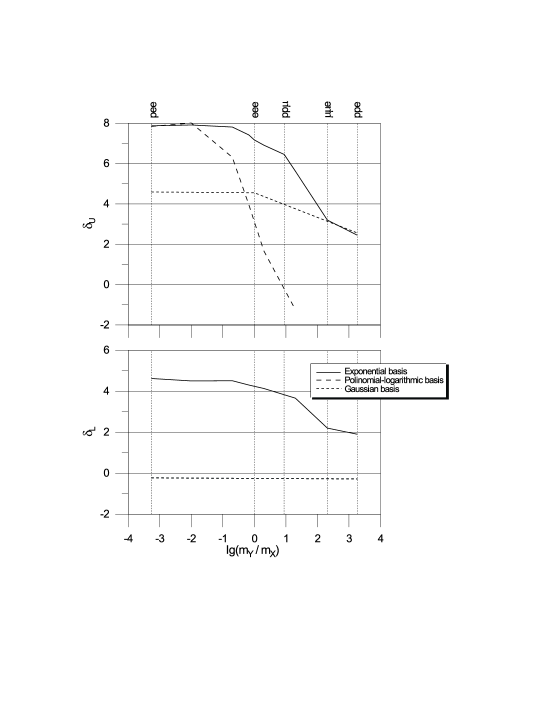
Figure 1: Dependence of $\delta_{U}$ and $\delta_{L}$ on mass ratio for Coulomb systems $X^{+}Y^{-}Y^{-}$

The composition of the majority of considered Coulomb systems with the particles of unit charge can be presented as $X^{\pm}Y^{\mp}Y^{\mp}$, the identical particles being denoted as $Y$. The binding energies decrease together with the values of masses but the accuracy of calculation depends only on the ratio of masses. For these systems the upper and lower bounds were calculated with $N=30$ in expansion (3), corresponding values $\delta_{U}$ and $\delta_{L}$ were plotted in Fig. 1 as the functions of mass ratio, $\xi_{YX}=m_{Y}/m_{X}$. In calculations of the lower bound the non-linear parameters were accepted to be equal to these found for the upper bound.

As expected, the increase of ratio $\xi_{YX}$ leads to the decrease of values $\delta_{U}$ and $\delta_{L}$ due to arising difficulties in description of motion of heavy particles. Nevertheless even at the approach to the two-center limit ($\xi_{YX}\gg 1$) the accuracy of calculations remains still satisfactory. For comparison, in Fig.1 the results of most detailed calculations with polynomial basis [8] are presented too. It is seen that the accuracy of calculations with polynomial basis [8] becomes bad for $\xi_{YX}>0.1$ in spite of large values of $N$. This comparison shows that the exponential basis is applicable for a wider range of values of $\xi_{YX}$ than the polynomial basis.

Note that in the case of Gaussian basis $\delta_{U}$ and $\delta_{L}$ decrease even more slowly than for exponential basis (see Fig.1) though the latter provides generally higher precision.

The exponential basis can be used as well in the case of nuclear systems, even inconvenient for calculation (weakly bounded systems, short-range attractive potentials with strong repulsion at small distances between particles, that can be identical or not identical). As a particularly ’inconvenient’ system hypertritium, ${}^{3}_{\Lambda}$H (consisting of $np\Lambda$), was chosen. For comparison a more ’convenient’ three-nucleon system, ³H, was considered. In these calculations two types of model nuclear $NN$-potentials were used, (i) purely attractive potential $NN-1$ and (ii) attractive potential with a soft core $NN-2$:

$$V_{NN}(r)=V_{r}(R_{r}/R)\exp(-R/R_{r})-V_{a}(R_{a}/R)\exp(-R/R_{a})$$ (4)

and attractive $\Lambda N$-potential:

$$V_{\Lambda N}(r)=-V_{a}\exp(-R/R_{a}),$$ (5)

the parameters $V_{a,r}$ and $R_{a,r}$ are given in Appendix B.

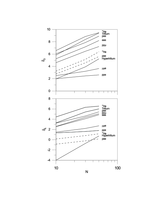
Figure 2: Dependence of $\delta_{U}$ and $\delta_{L}$ on number of terms in variational expansion for exponential basis

The convergence of the upper and lower estimates for exponential basis is illustrated in Table 1 and in Fig. 2 for various Coulomb and nuclear systems. As seen from Fig. 2 the dependence of $\delta_{U}$ and $\delta_{L}$ on the $\lg N$ is close to the linear one. In accordance with Fig. 1 the accuracy decreases as the system approaches to the adiabatic limit, and in parallel the convergence of variational estimates deteriorates (it is characterized by the slope of curves in Fig. 2). Note that the precision of calculations for considered nuclear systems is generally similar or even better than for Coulomb systems.

Besides, in Fig. 2 some results of calculations with the Gaussian basis are shown (dotted lines). It is seen that the convergence of the upper and lower bound is similar to that for exponential basis whereas the accuracy is significantly lower.

4 Comparison of results for different bases

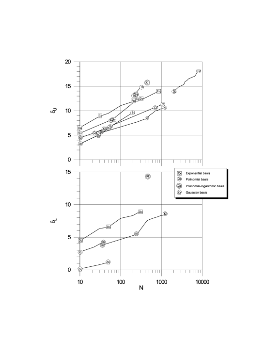
Figure 3: $\delta_{U}$ and $\delta_{L}$ in calculations of atom ^∞He with different variational expansions. Markers refer to the first author of the corresponding paper.

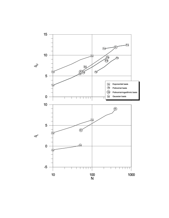
Figure 4: The same as in Fig. 3 but for hydrogen ion

Comparison of efficiency of different variational expansions is convenient to carry out on standard systems calculated by many authors. Such systems are ^∞He and ^∞H^- considered in [1]-[3],[5],[7]-[16]. In Fig. 3 the values of $\delta_{U}$ and $\delta_{L}$, are plotted for these papers where the most detailed calculations of atom ^∞He were carried out, the results of our calculations are presented there too. Similarly, in Fig. 4 $\delta_{U}$ and $\delta_{L}$ are presented for hydrogen ion ^∞H^-.

It is necessary to emphasize that both cases are examples of one-center systems. Therefore, this is a reason to expect that the expansions especially designed for one-center problems will gain the advantage. This is generally confirmed by our analysis. Up to present the most accurate many-parameters calculations of ^∞He were carried out using polynomial or polynomial-logarithmic bases. As it is seen from Fig. 3 and Fig. 4 the convergence of the variational expansions for these bases is generally better than for exponential or gaussian bases.

On the other hand, up to $\delta_{U}\approx 12$ the use of exponential basis is justified as it assures the same precision at lower number of terms (see Fig.3 and 4). Note that the over-high precision in non-relativistic calculations without taking into account relativistic and other corrections (that appears far before $\delta\approx 12$) have no physical meaning, though they are interesting from computational point of view.

As to the lower bound calculations they are rare in literature and we estimate the number of $N$ up to which the calculations of $E_{L}$ with exponential basis are justified (in the same sense as for $E_{U}$) as $100-200$.

Another limiting case is the adiabatic one (i.e. a two-center system with two heavy particles). In this case the use of polynomial basis leads to unsatisfactory results, and the exponential basis is evidently preferable (see Fig. 1). Moreover, the use of complex scale parameters in exponential basis increases significantly the accuracy of calculations [22]. The most accurate calculations of two-center systems were carried out in the framework of the Born-Oppenheimer approach [23] or its modifications [24], [25]. In particular, in paper [25] the energy of the system $H_{2}^{+}$ ($ppe^{-}$) was calculated with precision $\delta\approx 12$ but this is only some better than that of the calculation of [22] with exponential functions (note by the way that the number of basis terms in [22] was less than in [25]).

A more effective modification of exponential basis in two-center calculations is:

$$|a\rangle=\exp(-\alpha_{1}^{a}R_{1}-\alpha_{2}^{a}R_{2}-\alpha_{3}^{a}R_{3}-\beta^{a}R_{3}^{2}),$$ (6)

where $R_{3}$ is a distance between the heavy particles. Note that the dependence of this function on $R_{3}$ can be presented as $\exp(-\beta^{a}(R_{3}-R_{3}^{a})^{2})$, where $R_{3}^{a}$ is the new variational parameter connected with $\alpha_{3}^{a}$. Note that basis (6) is, in a certain sense, a particular case of ’carcass’ functions (constructed on the base of gaussians in paper [26]), whose use together with gaussians might be useful in nuclear physics for calculation with potentials changing the sign.

For functions (6) all the integrals needed for calculations of the upper variational bound are expressed in the closed form in terms of conventional functions. For instance, the basic integral can be calculated as:

$$G^{000}\equiv\int\limits_{0}^{\infty}e^{-x_{3}R_{3}-\beta R_{3}^{2}}dR_{3}\int\limits_{0}^{\infty}e^{-x_{2}R_{2}}dR_{2}\int\limits_{\mid R_{2}-R_{3}\mid}^{R_{2}+R_{3}}e^{-x_{1}R_{1}}dR_{1}=-\frac{1}{\sqrt{\beta}}\frac{F\Big{(}\frac{x_{1}+x_{3}}{2\sqrt{\beta}}\Big{)}-F\Big{(}\frac{x_{2}+x_{3}}{2\sqrt{\beta}}\Big{)}}{x_{1}^{2}-x_{2}^{2}},$$ (7)

where $F(z)\equiv e^{z^{2}}\int_{z}^{\infty}e^{-t^{2}}dt$.

The calculations of the ground state of the system $ppe^{-}$ with this modified basis lead to significantly better results than with purely exponential or gaussian bases. In particular, in our calculations it has been shown that even a single function (6) provides a better precision than 50 exponents or gaussians. Moreover, the basis (6) is more flexible than the exponential basis with complex parameters used in [22]. For instance, the result of calculations with $N=20$ for $ppe^{-}$ turns out to be better than that of paper [22] with 200 complex exponents (1400 variational parameters) and better than calculations with 300 functions for systems $\mu^{+}\mu^{+}e^{-}$, $dde^{-}$ and $tte^{-}$.

In addition to the preceding discussion of two limiting cases (one- and two-center problem) it is necessary to indicate that there exists a large region of values of $\xi_{YX}$ between $10^{-2}$ and $10^{2}$ where the exponential basis is beyond compare. Note that this is the region where the great part of known three-particle Coulomb systems is located. Thus, apart from gaussians, the exponential basis seems to be the most universal one in comparison with other approaches, applicable equally well to Coulomb and nuclear three-particle systems.

5 Stability of Coulomb Systems

All considered above Coulomb systems except two ($\alpha e^{-}e^{-}$ and $\alpha\mu^{-}e^{-}$) had summary charge $\pm 1$ and consisted of three single-charged particles from which two are identical. All systems of such type are stable in respect to separation of one of the particles. However this is not the case for other type of three particle Coulomb systems. For analysis of stability of Coulomb systems and for calculation of their energy it is natural to use the variational procedure with exponential basis as it is most universal in respect to masses of particles (see also [27]).

In general case the structure of a Coulomb system of three single-charged particles with total charge $\pm 1$ may be presented in the form $X^{\pm}Y^{\mp}Z^{\mp}$ where $m_{Y}\leq m_{Z}$. The stability of the system depends on two ratios of masses, $\xi_{YX}=m_{Y}/m_{X}$ and $\xi_{ZX}=m_{Z}/m_{X}$. A boundary delimiting the regions of stable and unstable systems is determined from the condition of coincidence of the energy of the three-particle system with that of the two-particle system $X^{\pm}Z^{\mp}$. The corresponding equation determining the interdependence between $\xi_{YX}$ and $\xi_{ZX}$ can be written as:

$$f(\xi_{YX},\xi_{ZX})\equiv\frac{E(X^{\pm}Y^{\mp}Z^{\mp})}{E(X^{\pm}Z^{\mp})}-1=0$$ (8)

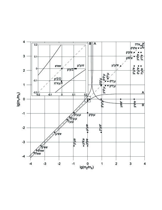
Figure 5: Boundary of stability for 3-particle Coulomb systems.

The solution of this equation is presented in Fig. 5 by the curve A. It is seen that not only systems with two identical particles are stable but also two-center systems (two heavy particles with identical charges plus light particle with opposite charge). In contrast, a system containing two heavy particles of opposite charges are unstable. An exception can occur if all three particles have nearly equal masses. This takes place for instance for exotic systems $p^{+}p^{-}\Sigma^{\pm}$ ($\xi_{YX}=1$, $\xi_{ZX}=1.2749$), $\mu^{+}\mu^{-}\pi^{\pm}$ ($\xi_{YZ}=1$, $\xi_{ZX}=1.3213$) and $\pi^{+}\pi^{-}\mu^{\pm}$ ($\xi_{YX}=0.7568$, $\xi_{ZX}=1$) for which $f=0.008745$, 0.006069 and 0.002354, respectively. Of course, a three-particle system which is stable with respect to emission of one of the constituent particles can be unstable in the excited state. This problem was considered in [4] for symmetric ($XYY$) systems with $m_{Y}/m_{X}\ll 1$.

For the case of systems of the type $X^{+m}Y^{+m}Z^{-m}$ containing multiple-charged particles the situation is quit similar to the case of single-charged particles considered above. Among three-body systems containing single and double charged particles the systems of the type $X^{++}Y^{-}Z^{+}$ and $X^{++}Y^{-}Z^{++}$ are unstable at any ratio of their masses, whereas the systems $X^{++}Y^{-}Z^{-}$ are always stable. As to the systems of the type $X^{++}Y^{--}Z^{+}$ they can be stable only for restricted values of ratios of their masses. The corresponding boundary is shown in the same Fig. 5, curve B.

Appendix A Standard integrals

A calculation of matrix elements of the Hamiltonian and its square reduces to the evaluation of the following integrals:

$$I^{klm}(x_{1},x_{2},x_{3})\equiv 8\pi^{2}\int\limits_{0}^{\infty}R_{1}^{k}dR_{1}\int\limits_{0}^{\infty}R_{2}^{l}dR_{2}\int\limits_{\mid R_{1}-R_{2}\mid}^{R_{1}+R_{2}}R_{3}^{m}dR_{3}\exp\Big{(}-\sum\limits_{p=1}^{3}x_{p}R_{p}\Big{)}.$$ (9)

The integrals $I^{klm}(x_{1},x_{2},x_{3})$ with non-negative indexes are the uniform polynomials of the $(k+l+m+3)$-th degree with respect to the variables $A_{i}\equiv 1/(x_{1}+x_{2}+x_{3}-x_{i})$.

To calculate the upper variational estimate the following integrals are necessary:

$$\begin{array}[]{rcl}I^{000}&=&A_{1}A_{2}A_{3};\\ N&=&2I^{000}\Big{(}(A_{1}+A_{2})(A_{2}+A_{3})(A_{3}+A_{1})-A_{1}A_{2}A_{3}\Big{)};\vphantom{\Bigg{\}}}\\ G_{1}&=&I^{000}(A_{1}A_{2}+A_{2}A_{3}+A_{3}A_{1}+2A_{1}^{2});\\ T_{1}&=&I^{111}-4I^{000}A_{2}A_{3}(A_{2}+A_{3}).\vphantom{\Bigg{\}}}\end{array}$$

(Here and further an unimportant numerical factor $16\pi^{2}$ is dropped.)

For presentation of the integrals (9) with negative indexes it is convenient to use the following notations:

$$\begin{array}[]{c}B_{1}\equiv(x_{2}-x_{3})^{-1},\hskip 28.45274ptB_{2}\equiv(x_{3}-x_{1})^{-1},\hskip 28.45274ptB_{3}\equiv(x_{1}-x_{2})^{-1};\\ S_{C1}^{[n]}=B_{1}^{n}\ln\frac{A_{2}}{A_{3}}-B_{1}^{n-1}A_{3}-\cdots-\frac{\textstyle 1}{\textstyle n-1}B_{1}A_{3}^{n-1};\vphantom{\Bigg{\}}}\\ S_{E1}^{[n]}=B_{1}^{n}\ln\frac{A_{2}}{A_{3}}-B_{1}^{n-1}A_{2}+\cdots+\frac{(-1)^{n-1}}{n-1}B_{1}A_{2}^{n-1};\\ S_{1}^{[n]}=S_{C1}^{[n]}+S_{E1}^{[n]};\vphantom{\Bigg{\}}}\\ N_{1}^{[n]}=\frac{\textstyle 1}{\textstyle n}\Big{(}A_{3}^{n}\ln\frac{A_{1}}{A_{2}}+A_{2}^{n}\ln\frac{A_{1}}{A_{3}}-S_{C3}^{[n]}+(-1)^{n-1}S_{E2}^{[n]}\Big{)}.\end{array}$$

To calculate the lower variational estimate the following integrals are necessary:

$$\begin{array}[]{ccl}J_{12}=J_{21}&=&I^{000}(A_{1}+A_{2});\vphantom{\Bigg{\}}}\\ J_{11}&=&A_{1}^{3}S_{1}^{[1]}-A_{1}S_{1}^{[3]}+I^{000}\Big{(}A_{1}/2+(A_{1}+A_{2}+A_{3})/2\Big{)};\\ \\ W_{12}&=&I^{000}A_{1}(A_{3}+2A_{2})+2A_{2}^{3}S_{2}^{[2]}-2A_{2}^{2}S_{2}^{[3]};\vphantom{\bigg{\}}}\\ W_{21}&=&I^{000}A_{2}(A_{3}+2A_{1})-2A_{1}^{3}S_{1}^{[2]}-2A_{1}^{2}S_{1}^{[3]};\vphantom{\Bigg{\}}}\\ W_{11}&=&G_{1}-2I^{000}A_{2}A_{3};\\ \\ Q_{12}=Q_{21}&=&N-4I^{000}A_{3}(A_{1}^{2}+A_{2}^{2})-8A_{k}^{3}S_{3}^{[3]};\vphantom{\Bigg{\}}}\\ Q_{11}&=&3A_{2}\Big{(}-2S_{E2}^{[1]}A_{2}^{4}+3S_{E2}^{[2]}A_{2}^{3}-3S_{E2}^{[4]}A_{2}+2S_{E2}^{[5]}\Big{)}+\\ &+&3A_{3}\Big{(}-2S_{C3}^{[1]}A_{3}^{4}-3S_{C3}^{[2]}A_{3}^{3}\vphantom{\Bigg{\}}}+3S_{C3}^{[4]}A_{3}+2S_{C3}^{[5]}\Big{)}+\\ &+&(2T_{1}-N)+I^{5-1-1}/4;\end{array}$$

$$\begin{array}[]{rcl}I^{5-1-1}&=&60\Bigg{\{}x_{1}^{-1}\Big{[}N_{1}^{[5]}-A_{2}A_{3}\Big{(}A_{2}^{3}/4+A_{2}^{2}A_{3}/6+A_{2}A_{3}^{2}/6+A_{3}^{3}/4\Big{)}\Big{]}+\\ &+&x_{1}^{-2}\Big{[}N_{1}^{[4]}-\vphantom{\Bigg{\}}}A_{2}A_{3}\Big{(}A_{2}^{2}/3+A_{2}A_{3}/4+A_{3}^{2}/3\Big{)}\Big{]}+\\ &+&x_{1}^{-3}\Big{[}N_{1}^{[3]}-A_{2}A_{3}\Big{(}A_{2}/2+A_{3}/2\Big{)}\Big{]}+x_{1}^{-4}\Big{[}N_{1}^{[2]}-A_{2}A_{3}\Big{]}+\vphantom{\Bigg{\}}}x_{1}^{-5}N_{1}^{[1]}+\\ &+&x_{1}^{-6}\Big{[}\mathop{\rm Li_{2}}\nolimits(1-\frac{A_{2}}{A_{1}})+\mathop{\rm Li_{2}}\nolimits(1-\frac{A_{3}}{A_{1}})+\frac{1}{2}\ln^{2}\frac{A_{2}}{A_{3}}+\frac{\pi^{2}}{6}\Big{]}\Bigg{\}}.\end{array}$$

The expression for $I^{5-1-1}$ contains the di-logarithmic function $\mathop{\rm Li_{2}}\nolimits(z)\equiv-\int_{0}^{z}t^{-1}\ln(1-t)dt$. If $u=x_{1}/x_{2}$ and $v=x_{1}/x_{3}$ are simultaneously small one can use for it the expansion:

$$I^{5-1-1}=x_{2}^{-6}\sum\limits_{n=0}^{\infty}u^{n}P_{n+5}(w)\frac{(n+5)!}{n!(n+6)}+x_{3}^{-6}\sum\limits_{n=0}^{\infty}v^{n}P_{n+5}(w^{-1})\frac{(n+5)!}{n!(n+6)}$$

$$P_{q}(\alpha)=P_{q-2}(\alpha)-\frac{(-\alpha)^{q}}{q},\hskip 11.38109ptq=2,3,\cdots,\hskip 11.38109ptP_{0}=-\ln(1+\alpha),\hskip 11.38109ptP_{1}=1,\hskip 11.38109ptw=\frac{v}{u}.$$

These formulas are used if $\max(u,v)<0.3$.

Appendix B Model Nuclear potentials

Parameters of used nuclear model potentials (4) and (5) are given in Table 4.

In calculations of hypertritium $NN$-potentials $NN$-1 and $NN$-2 were used. The radial parameter of purely attractive potential $NN$-1 was chosen corresponding to one-pion exchange whereas for $NN$-2 potential the values of $R_{r}$ and $R_{a}$ were adopted from paper [28]. The depth parameters for potentials $NN$-1 and $NN$-2 were matched to correct deuteron energy, additional experimental data in fitting of parameters for $NN$-2 potential were deuteron radius and phases of S-wave triplet $np$-scattering up to energy 300 MeV. In calculations of tritium ³H the potential $NN$-3 was used with the same radial parameter as for potential $NN$-1, whereas depth parameters was chosen to describe the correct tritium binding energy in calculations with $N=100$ in expansion (3).

The radius of $\Lambda N$-potential was adopted from paper [29] while the depth parameter provided the correct hypertritium binding energy (B_Λ = 0.13 MeV) in calculations with $N=100$.

System	N	$E_{U}$, au	$E_{L}$, au	Comment
${}^{\infty}He$	10	-2.903 723 6	-2.903 83
	30	-2.903 724 373 0	-2.903 725 8
	50	-2.903 724 375 9	-2.903 725 2
	100	-2.903 724 377 009	-2.903 724 414
	200	-2.903 724 377 030 3	-2.903 724 391
	300	-2.903 724 377 033 2	-2.903 724 380
$\alpha ee$	300	-2.903 304 557 732 3	-2.903 304 561	$m_{\alpha}=7294.2996m_{e}$
${}^{\infty}H^{-}$	10	-0.527 750 546	-0.528 062
	30	-0.527 751 009 425	-0.527 764
	50	-0.527 751 015 895	-0.527 752 977
	100	-0.527 751 016 400	-0.527 751 663
$pee$	100	-0.527 445 880 971	-0.527 446 533	$m_{p}=1836.1527m_{e}$
$\mu ee$	100	-0.525 054 806 098	-0.525 055 501	$m_{\mu}=206.768262m_{e}$
$Ps^{-}$	10	-0.262 003 563	-0.262 744
	30	-0.262 005 053	-0.262 026
	50	-0.262 005 068 6	-0.262 008 7
$pp\mu$	10	-0.494 374	-0.495 7	In meso-atomic units
	30	-0.494 386 645	-0.494 408	$m_{p}=8.8802444m_{\mu}$
	50	-0.494 386 790	-0.494 391 1
$dd\mu$	10	-0.531 044	-0.534 4	In meso-atomic units
	30	-0.531 109 463	-0.531 241	$m_{d}=17.7516751m_{\mu}$
$tt\mu$	10	-0.546 224	-0.551 2	In meso-atomic units
	30	-0.546 371 871	-0.546 517	$m_{t}=26.5849388m_{\mu}$
$\mu\mu e$	10	-0.583 276	-0.604 5
	30	-0.584 757	-0.588 82
	50	-0.584 995	-0.586 267
	20	-0.585 126 081 8		’Carcass’ basis
$ppe$	10	-0.591 03	-0.625
	30	-0.595 02	-0.612
	50	-0.595 67	-0.606
	20	-0.597 139 058 5		’Carcass’ basis
$dde$	10	-0.591 38	-0.621
	30	-0.596 06	-0.610
	20	-0.598 788 780 3		’Carcass’ basis
$tte$	10	-0.591 59	-0.615
	30	-0.596 34	-0.608
	20	-0.599 506 906 3		’Carcass’ basis
$p\mu e$	10	-0.584 18	-0.645
$\alpha\mu e$	10	-1.947 287 542	-1.947 429	In meso-atomic units
	30	-1.947 287 553 22	-1.947 290 320	$E_{0}=$-1.947 287 553 40, $m_{\alpha}=35.2776559m_{\mu}$, $m_{e}=0.00483633218m_{\mu}$
${}^{3}_{\Lambda}$H	50	-2.359 478 5	-2.437 6	Potentials NN-1 and $\Lambda$N-1; energies are in MeV
${}^{3}_{\Lambda}$H	50	-2.358 597 8	-2.808	Potentials NN-2 and $\Lambda$N-2; energies are in MeV
3H	50	-8.480 037 312	-8.480 045 6	Potential NN-3; energies are in MeV

Table 1: Upper and lower bounds for Coulomb and nuclear systems

Variant	$V_{r}$, MeV	$R_{r}$, Fm	$V_{a}$, MeV	$R_{a}$, Fm
NN-1	0	0	50.6414	1.4
NN-2	2719.20	0.32	730.24	0.65
NN-3	0	0	40.0419	1.4
$\Lambda$N-1	0	0	687.00	0.23
$\Lambda$N-2	0	0	711.00	0.23

Table 2: Parameters of nuclear model potentials

^∞H^-

References

- [1] Schwartz C.: Phys.Rev. 128, 1147 (1962)
- [2] Thakkar A.J., Koga T.: Phys.Rev. A50, 854 (1994)
- [3] Frankowski K., Pekeris C.L.: Phys.Rev. 146, 46 (1966)
- [4] Frolov A.M.: J.Phys. B: At.Mol.Opt.Phys. 25, 3059 (1992)
- [5] Kolesnikov N.N., Tarasov V.I.: J.Nucl.Phys. 35, 609 (1982)
- [6] Usukura J., Varga K., Suzuki Y.: Phys.Rev. A58, 1918 (1998)
- [7] Donchev A.G., Kolesnikov N.N., Tarasov V.I.: Phys. At. Nucl. 63, 419 (2000)
- [8] Kleindienst H., Emrich R.: Int.J.Quant.Chem. 37, 257 (1990)
- [9] Kinoshita T.: Phys.Rev. 105, 1490 (1957)
- [10] Pekeris C.L.: Phys.Rev. 126, 1470 (1962)
- [11] Thakkar A.J., Smith V.H., Jr: Phys.Rev. A15, 1 (1977)
- [12] Kleindienst H., Wolfgang M.: Theoret.Chim.Acta. 56, 183 (1980)
- [13] Freund D.E., Huxtable B.D., Morgan III J.D.: Phys.Rev. A29, 980 (1984)
- [14] Cox H., Smith S.J., Sutcliffe B.T.: Phys.Rev. 49, 4520 (1994); ibid 49, 4533 (1994)
- [15] Goldman S.P.: Phys.Rev. A57, 677 (1998)
- [16] Frolov A.M.: Phys.Rev. A58, 4479 (1998)
- [17] Komasa J., Cencek W., Pychlewski J.: Phys.Rev. A52, 4500 (1995)
- [18] Frolov A.M., Smith V.H., Jr.: Phys.Rev. A55, 2662 (1997)
- [19] Yan Z.-C., Tambasco M., Drake G.W.: Phys.Rev. A57, 1652 (1998)
- [20] Yan Z.-C., Ho Y.K.: Phys.Rev. A59, 2697 (1999)
- [21] Frolov A.M.: Phys.Rev. A60, 2834 (1999)
- [22] Frolov A.M.: Phys.Rev. A57, 2436 (1998); ibid A59, 4270 (1999)
- [23] Born M., Oppenheimer J.R.: Ann.Phys. 84, 457 (1927)
- [24] Ponomarev L.I.: J.Phys. B14, 591 (1981)
- [25] Gremaud B., Dominique D., Billy N.: J.Phys. B31, 383 (1998)
- [26] Zakharov P.P., Kolesnikov N.N., Tarasov V.I.: Vestn.Mosk.Univ. Ser.3: Fiz,Astron. 24, 34 (1983), in russian
- [27] Frolov A.M., Smith V.H., Jr. V.H.: J.Phys. B: At.Mol.Opt.Phys. 28, L449 (1995)
- [28] Malfliet R.A., Tjon J.A.: Nucl.Phys. A127, 161 (1969)
- [29] Kolesnikov N.N., Tarasov V.I.: Vestn.Mosk.Univ. Ser.3: Fiz,Astron. 18, 8 (1977), in russian