Anomalous Capacitive Sheath with Deep Radio Frequency Electric Field Penetration

Abstract

A novel nonlinear effect of anomalously deep penetration of an external radio frequency electric field into a plasma is described. A self-consistent kinetic treatment reveals a transition region between the sheath and the plasma. Because of the electron velocity modulation in the sheath, bunches in the energetic electron density are formed in the transition region adjusted to the sheath. The width of the region is of order $V_{T}/\omega$, where $V_{T}$ is the electron thermal velocity, and $\omega$ is frequency of the electric field. The presence of the electric field in the transition region results in a cooling of the energetic electrons and an additional heating of the cold electrons in comparison with the case when the transition region is neglected.

PACS numbers:52. 35.Mw, 52.65Ff, 52.65-y, 52.75-d, 52.80.Pi

The penetration of the electric field perpendicular to the plasma boundary was studied by Landau in the linear approximation [1]. He showed that an external electric field with amplitude $E_{0}$ is screened by the plasma electrons in the sheath region in a distance of order the Debye length, and reaches a value $E_{0}/\varepsilon$ in the plasma, where $\varepsilon$ is plasma dielectric constant. In many practical applications, the value of the external electric field is large: the potential drop in the sheath region $V_{sh}$ is typically of order hundreds of Volts and is much larger than electron temperature $T_{e}$, which is of order of a few Volts; and the field penetration has to be treated nonlinearly. The asymptotic solution of sheath structure has been studied by Lieberman in the limit $V_{sh}>>T_{e}$ [2]. In this treatment, the plasma sheath boundary is considered to be infinitely thin and the position of the boundary is determined by the condition that the external electric field is screened in the sheath regions when electrons are absent. Electron interactions with the sheath electric field are traditionally treated as collisions with a moving potential barrier (wall). It is well known that multiple electron collisions with an oscillating wall result in electron heating, provided there is sufficient phase-space randomization in the plasma bulk. It is common to describe the sheath heating by considering the electrons as test particles, and neglecting the plasma electric fields [3]. Kaganovich and Tsendin proved in Ref.[4] that accounting for the electric field in the plasma reduces the electron sheath heating, and the electron sheath heating vanishes completely in the limit of uniform plasma density. Therefore, an accurate description of the rf fields in the bulk of the plasma is necessary for calculating the sheath heating. The electron velocity is oscillatory in the sheath, and as a result of this velocity modulation electron density bunches appear in the region adjusted to the sheath. The electron density perturbations decay due to phase mixing over a length of order $V_{T}/\omega,$ where $V_{T}$ is the electron thermal velocity, and $\omega$ is the frequency of the electric field. The electron density perturbations polarize the plasma and produce an electric field in the plasma bulk. This electric field, in turn, changes the velocity modulation and correspondingly influences the electron density perturbations. Therefore, electron sheath heating has to be studied in a self-consistent nonlocal manner assuming a finite temperature plasma.

Notwithstanding the fact, that particle-in-cell simulations results are widely available for the past decade [5-7] a basic understanding of the electron sheath heating is incomplete, because no one has studied the electric field in the plasma bulk using a nonlocal approach, similar to the anomalous skin effect for inductive electric field [8]. In this regard, analytical models are of great importance because they shed light on the most complicated features of collisionless electron interactions with the sheath. In this Letter, an analytical model is developed to explore the effects associated with the self-consistent non-local nature of the phenomenon.

One of the approaches to study electron sheath heating is based on a fluid description of the electron dynamics. For the collisionless case, closure assumptions for the viscosity and heat fluxes are necessary. In most cases, the closure assumptions are made empirically or phenomenologically [6, 7]. The closure assumptions have to be justified by direct comparison with the results of kinetic calculations as is done, for example, in Ref. [9]. Otherwise, inaccurate closure assumptions may lead to misleading results as discussed below.

To model the sheath-plasma interaction analytically, the following simplifying assumptions have been adopted. The discharge frequency is assumed to be small compared with the electron plasma frequency. Therefore, most of the external electric field is screened in the sheath region by an ion space charge. The ion response time is typically larger than the inverse discharge frequency, and the ion density profile is quasi-stationary. There is an ion flow from plasma bulk towards electrodes. In the sheath region, ions are being accelerated towards the electrode by the large sheath electric field, and, the ion density in the sheath region is small compared with the bulk ion density. In the present treatment, the ion density profile is assumed fixed and is modeled in a two-step approximation: the ion density $n_{b}$ is uniform in the plasma bulk, and the ion density in the sheath $n_{sh}<n_{b}$ is also uniform (see Fig.1). At the sheath-plasma boundary, there is a stationary potential barrier for the electrons ($e\Phi_{sh}$), so that only the energetic electrons reach the sheath region. The potential barrier is determined by the quasineutrality condition, i.e., when the energetic electrons enter the sheath region, their mean density is equal to the ion density [$n_{e}(\Phi_{sh})=n_{sh}$].

The electron density profile is time-dependent in response to the time-varying sheath electric field. The large sheath electric field does not penetrate into the plasma bulk. Therefore, the quasineutrality condition holds in the plasma bulk, i.e., the electron density is equal to ion density, $n_{e}=n_{b}.$ In the sheath region, the electrons are reflected by the large sheath electric field. Therefore, $n_{e}=n_{sh}$ for $x>x_{sh}(t)$, and $n_{e}=0$ for $x<x_{sh}(t)$, where $x_{sh}(t)$ is the position of the plasma-sheath boundary [2]. From Maxwell’s equations it follows that ${\bf\nabla\cdot J}=0$, where the total current ${\bf J}$ is the sum of the displacement current and the electron current. In the one-dimensional case, the condition ${\bf\nabla\cdot J}=0$ yields the conservation of the total current:

$$en_{e}V_{e}+\frac{1}{4\pi}\frac{\partial E_{sh}}{\partial t}=j_{0}\sin(\omega t+\phi),$$ (1)

where $j_{0}$ is the amplitude of the rf current controlled by the external circuit and $\phi$ is the initial phase. In the sheath, electrons are absent in the region of large electric field, and the Eq.(1) can be integrated to give [4]

$$E_{sh}(x,t)=\frac{4\pi j_{0}}{\omega}[-1-\cos(\omega t+\phi)]+4\pi|e|n_{sh}x,\quad x<x_{sh}(t)$$ (2)

where Poisson’s equation has been used to determined the spatial dependence of the sheath electric field. The first term on the right-hand side of Eq.(2) describes the electric field at the electrode, the second term relates to ion space charge screening of the sheath electric field. The position of the plasma-sheath boundary $x_{sh}(t)$ is determined by the zero of the sheath electric field, $E_{sh}[x_{sh}(t),t]=0$. From Eq.(2) it follows that

$$x_{sh}(t)=\frac{V_{sh0}}{\omega}[1+\cos(\omega t+\phi)],$$ (3)

where $V_{sh0}=j_{0}/(en_{sh})$ is the amplitude of the plasma-sheath boundary velocity. The ion flux on the electrode is small compared with the electron thermal flux. Because electrons attach to the electrode, the electrode surface charges negatively, so that in a steady-state discharge, the electric field at the electrode is always negative, preventing an electron flux on the electrode. However, for a very short time ($\omega t_{n}+\phi\approx\pi(1+2n)$) the sheath electric field vanishes, allowing electrons to flow to the electrode for compensation of the ion flux. Note that there is a large difference between the sheath structure in the discharge and the sheath for obliquely incident waves interacting with a plasma slab without any bounding walls. Because electrodes are absent, electrons can move outside the plasma, and the electric field in the vacuum region, $E_{sh}(x,t)=(4\pi j_{0}/\omega)\cos(\omega t+\phi)$, may have a different sign. Therefore, electrons may penetrate into the region of large electric field during time when $E_{sh}(x,t)<0$ [10,11]. However, in the discharge, because the sheath electric field given by Eq.(2) is always reflecting electrons, the electrons never enter the region of the large sheath electric field, which is opposite to the case of obliquely incident waves.

The calculations based on the two-step ion density profile model is known to yield discharge characteristics in good agreement with experimental data and full-scale simulations [12].

Throughout this paper, linear theory is used because the plasma-sheath boundary velocity and the mean electron flow velocity are small compared with the electron thermal velocity [4,5]. The important spatial scale is the length scale for phase mixing, $l_{mix}=V_{T}/\omega$. The sheath width satisfies $2V_{sh0}/\omega<<l_{mix}$ because $V_{sh}<<V_{T}$. Therefore, the sheath width is neglected, and electron interactions with the sheath electric field are treated as a boundary condition. The collision frequency ($\nu$) is assumed to be much less than the discharge frequency ($\nu<<\omega$), and correspondingly the mean free path is much larger than the length scale for phase mixing. Therefore, the electron dynamics is assumed to be collisionless. The discharge gap is considered to be sufficiently large compared with the electron mean free path, so that the influence of the opposite sheath is neglected. The effects of finite gap width are discussed in Ref. [13].

The electron interaction with the large electric field in the sheath is modelled as collisions with a moving oscillating rigid barrier with velocity $V_{sh}(t)=dx_{sh}(t)/dt$. An electron with initial velocity $-u$ after a collision with the plasma-sheath boundary - modeled as a rigid barrier moving with velocity $V_{sh}(t)$ - acquires a velocity $u+2V_{sh}$. Therefore, the power deposition density transfer from the oscillating plasma-sheath boundary is given by [2]

$$P_{sh}=\frac{m}{2}\left\langle\int_{-V_{sh}}^{\infty}du\left[u+V_{sh}(t)\right]\left[(2V_{sh}(t)+u)^{2}-u^{2}\right]\,f_{sh}(-u,t)\right\rangle,$$ (4)

where $m$ is the electron mass, $f_{sh}(-u,t)$ is the electron velocity distribution function in the sheath, and $\left\langle\cdot\cdot\cdot\right\rangle$ denotes a time average over the discharge period. Introducing a new velocity distribution function $g(-u^{\prime},t)=f_{sh}[-u-V_{sh}(t),t]$, Eq.(4) yields

$$P_{sh}=-2m\left\langle V_{sh}(t)\int_{0}^{\infty}u^{\prime 2}g(-u^{\prime},t)du^{\prime}\right\rangle,$$ (5)

where $-u^{\prime}=-u-V_{sh}$ is the electron velocity relative to the oscillating rigid barrier. From Eq.(5) it follows that, if the function $g(u^{\prime})$ is stationary, then ($P_{sh}=0$) there is no collisionless power deposition due to electron interaction with the sheath [7, 14]. For example, in the limit of a uniform ion density profile $n_{sh}=n_{b}$, $g(u^{\prime})$ is stationary (in an oscillating reference frame of the plasma-sheath boundary), and the electron heating vanishes [4]. Indeed, in the plasma bulk the displacement current is small compared with the electron current, and from Eq.(1) it follows that the electron mean flow velocity in the plasma bulk, $V_{b}(t)=-j_{0}\sin(\omega t+\phi)/|e|n_{b}$, is equal to the plasma-sheath velocity $V_{sh}(t)$, from Eq.(3). Therefore, the electron motion in the plasma is strongly correlated with the plasma-sheath boundary motion. From the electron momentum equation it follows that there is an electric field, $E_{b}=m/e\,dV_{b}(t)/dt$, in the plasma bulk. In a frame of reference moving with the electron mean flow velocity, the sheath barrier is stationary, and there is no force acting on the electrons, because the electric field is compensated by the inertial force ($eE_{b}-mdV_{b}(t)/dt=0)$. Therefore, electron interaction with the sheath electric field is totally compensated by the influence of the bulk electric field, and the collisionless heating vanishes [4].

The example of a uniform density profile shows the importance of a self-consistent treatment of the collisionless heating in the plasma. If the function $g(u^{\prime},t)$ is nonstationary, there is net power deposition. In this Letter, a kinetic calculation is performed to yield the correct electron velocity distribution function $g(u^{\prime},t)$ and, correspondingly, the net power deposition.

The electron motion is different for the low energy electrons with initial velocity in the plasma bulk $|u|<u_{sh}$, where $u_{sh}^{2}=2e\Phi_{sh}/m$, and for the energetic electrons with velocity $|u|>u_{sh}$. The low energy electrons with initial velocity in the plasma bulk $-u$ are reflected from the stationary potential barrier $e\Phi_{sh}$, and then return to the plasma bulk with velocity $u$. High energy electrons enter the sheath region with velocity $u_{1}=-(u^{2}-u_{sh}^{2})^{1/2}$. They have velocity $u_{2}=2V_{sh}-u_{1}$ colliding with the moving rigid barrier, and then return to the plasma bulk with velocity $(u_{2}^{2}+u_{sh}^{2})^{1/2}$ [15].

As the electron velocity is modulated in time during reflections from the plasma-sheath boundary, so is the energetic electron density (by continuity of electron flux). This phenomenon is identical to the mechanism for klystron operation [16]. The perturbations in the energetic electron density yield an electric field in the transition region adjusted to the sheath.

The electron velocity distribution function is taken to be a sum of a stationary isotropic part $f_{0}(u)$ and a nonstationary anisotropic part $f_{1}(x,u,t)$. $f_{1}$ is to be of the form $f_{1}(x,u,t)=f_{1}(x,u)\exp(-i\omega t)$. The linearized Vlasov equation becomes

$$-i\omega f_{1}+u\frac{\partial f_{1}}{\partial x}+\frac{eE(x)}{m}\frac{df_{0}}{du}=-\nu f_{1},$$ (6)

where the term on the right-hand side accounts for rare collisions ($\nu<<\omega$). All time-dependent variables are assumed to be harmonic functions of time, proportional to $\exp(-i\omega t),$ and, in the subsequent analysis, the multiplicative factor $\exp(-i\omega t)$ is omitted from the equations. The electron velocity distribution function must satisfy the boundary condition at the plasma-sheath boundary ($x=0$) corresponding to $f(0,u)=f(0,-u)$ for $|$$u|<u_{sh}$, and $f_{sh}(u^{\prime})=f_{sh}(2V_{sh}-u^{\prime}),$ for $u>u_{sh}$, where $u^{\prime}=(u^{2}-u_{sh}^{2})^{1/2}$  and $f_{sh}$ is the electron velocity distribution in the sheath. From energy and flux conservation, $u^{\prime}f_{sh}(u^{\prime})du^{\prime}=uf(u)du$, it follows that $f_{sh}(u^{\prime})=f[(u^{\prime 2}+u_{sh}^{2})^{1/2}]$. Linearly approximating the boundary conditions yields

$$f_{1}(0,u)=f_{1}(0,-u),\,\quad 0<u<u_{sh},$$ (7)

$$f_{1}(0,u)=f_{1}(0,-u)+2V_{sh}\frac{u^{\prime}}{u}\frac{df_{0}}{du}\,,\quad u>u_{sh}.$$ (8)

The electric field is determined from the condition of conservation of the total current ($j_{0}$), which gives

$$e\int_{-\infty}^{\infty}uf_{1}(x,u)du-\frac{i\omega}{4\pi}E(x)=j,$$ (9)

where $j=\,j_{0}e^{i(\phi+\pi/2)}$, and the first term is the electron current and the second term corresponds to a small displacement current. Equations (6) and (9), together with the boundary conditions (7), (8) comprise the full system of equations for the bulk plasma.

It is convenient to solve Eq. (6) by continuation into the region $x<0$. First, we introduce the artificial force

$$F(x,u)=2mV_{sh}u^{\prime}\delta(x)\Theta(|u|-u_{sh}),$$ (10)

where $V_{sh}=j/en_{sh}$, $\delta(x)$ is the Dirac delta-function, and $\Theta(u)$ is the Heaviside step function. The force in Eq.(10) accounts for the change of the energetic electron velocity in the sheath region. Equation (6) together with the boundary conditions (7) and (8) are equivalent to Eq. (6) with the force in Eq.(10) added to the third term of Eq. (6). This gives

$$-i\omega f_{1}+u\frac{\partial f_{1}}{\partial x}+\frac{eE(x)+F(x,u)}{m}\frac{df_{0}}{du}=-\nu f_{1},$$ (11)

where the boundary condition (7) for all electrons becomes

$$f_{1}(0,u)=f_{1}(0,-u).$$ (12)

In this formulation, the half-space problem is equivalent to that of an infinite medium in which the electric field is antisymmetric about the plane $x=0$, with $E(x)=-E(-x)$ [1, 17]. Such a continuation makes Eq. (11) invariant with respect to the transformation $x\rightarrow-x$, and $u\rightarrow-u$. Electrons reflected from the boundary in the half-space ($x>0$) problem correspond to electrons passing freely through the plane $x=0$ from the side $x<0$ in the infinite-medium problem.

A spatial Fourier the transform of Eq. (11) gives

$$f_{1}(k)=\frac{eE(k)+F_{sh}(u)}{mi(\omega-uk+i\nu)}\frac{df_{0}}{du},$$ (13)

where $E(k)$ is the Fourier transform of $E(x)$

$$E(k)=\int_{-\infty}^{\infty}E(x)\exp(-ikx)dx,$$ (14)

and $F_{sh}(u)=2mV_{sh}u^{\prime}\Theta(|u|-u_{sh}).$ It is convenient to divide the electric field in the plasma into two parts corresponding to $E(x)=E_{1}(x)+E_{b}sgn(x)$, where $E_{1}(x)\rightarrow 0$ for $x\rightarrow\infty$, and $E_{b}$ is the value of the electric field far away from the sheath region. The Fourier transform of the electron current can be obtained by integrating Eq. (13) over velocity, yielding

$$j(k)=\sigma(k)E_{1}(k)-\frac{2i}{k}\left[E_{sh}\sigma_{sh}(k)+\sigma(k)E_{b}\right],$$ (15)

$$\sigma(k)=-\frac{ie^{2}}{m}\int_{-\infty}^{\infty}\frac{u}{(\omega-uk+i\nu)}\frac{df_{0}}{du}du,$$ (16)

$$\sigma_{sh}(k)=\frac{ie^{2}k}{(\omega+i\nu)m}\int_{-\infty}^{\infty}\frac{uu^{\prime}\Theta(|u|-u_{sh})}{(\omega-uk+i\nu)}\frac{df_{0}}{du}du,$$ (17)

where $\sigma(k)$ is the electron conductivity, $\sigma_{sh}(k)$ is the effective conductivity due to electron interaction with the sheath, and $E_{sh}=(-i\omega+\nu)mV_{sh}/e$ is the effective electric field corresponding to $V_{sh}$.

The Fourier amplitude $E_{1}(k)$ is to be determined from Eq.(9) continued into the half-space $x<0$. Because $E(x)$ is an antisymmetric function about the plane $x=0$, $j_{0}$ is continued with negative sign into the half-space $x<0$, and the Fourier transform of $j_{0}sgn(x)$ is $-2i\,j_{0}/k$. Substituting $E(k)=E_{1}(k)-2iE_{b}/k$ and $j_{0}=\left[\sigma(0)-i\omega/4\pi\right]E_{b}$ into Fourier transform of Eq.(9) gives

$$E_{1}(k)=-\frac{2i}{k}\frac{[\sigma(0)-\sigma(k)]E_{b}-E_{sh}\sigma_{sh}(k)}{\sigma(k)-\frac{i\omega}{4\pi}}.$$ (18)

Notice that, if the plasma density in the sheath is equal to the bulk density $n_{sh}=n_{b}$, then $u_{sh}=0$, $E_{b}=E_{sh}$ and $\sigma(0)-\sigma(k)=\sigma_{sh}(k)$. Therefore, $E_{1}(k)=0$ and the uniform electric field $E_{b}$ satisfies the current conservation condition, as discussed earlier.

The profile for $E_{1}(x)$ given by inverse Fourier transform

$$E(x)=\frac{1}{2\pi}\int_{-\infty}^{\infty}E(k)\exp(ikx)dk$$ (19)

is shown at the top in Fig.2. For $x<6V_{T}/\,\omega$ the electric field profile is close to $E_{1}(x)\approx E_{1}(0)\exp(-\lambda x\omega/V_{T}\,)$, where $E_{1}(0)=-0.72$, and $\lambda=0.19+0.77i$ for the conditions in Fig.2. For $x>6V_{T}/\,\omega$, the electric field profile is no longer a simple exponential function, similar to the case of the anomalous skin effect [17]. The three components of current corresponding to the first, second, and third terms in Eq. (15) are shown at the bottom in Fig.2. The first term describes the current ($j_{tr}$) driven by the electric field $E_{1}(x)$ under the assumption of specular reflection at the boundary. The second term relates the current ($j_{sh}$) of the energetic electrons owing only to a velocity change due to reflections from the large sheath electric field. The third term describes the current ($j_{b}$) driven by the uniform electric field $E_{b}$ under the assumption of specular reflection at the boundary. Due to the boundary condition of specular reflection in Eq. (7), both of the currents $j_{b}$ and $j_{tr}$ are equal to zero at $x=0$. Also, both of the currents $j_{tr}$ and $j_{sh}$ vanish at $x>15V_{T}/\,\omega$ due to phase mixing, and the only current left here is $j_{b}.$ In contrast to large $x$, at small $x<<V_{T}/\,\omega$ the total current is entirely due to energetic electrons interacting with the sheath $j_{sh}$. Indeed, the energetic electrons enter the sheath region with velocity distribution $f_{sh}(u^{\prime})$. The electron current is given by the sum of the contribution from the electrons approaching the oscillating barrier and from the electrons already reflected from the barrier, $j_{sh}=\int_{V_{sh}}^{\infty}u^{\prime}f_{sh}(u^{\prime})du^{\prime}+\int_{-\infty}^{-V_{sh}}u^{\prime}f_{sh}(u^{\prime})du^{\prime}.$ Because $f_{sh}(u^{\prime})=f_{sh}(2V_{sh}-u^{\prime})$,  $j_{sh}=2eV_{sh}\int_{V_{sh}}^{\infty}f_{sh}(u)du\approx eV_{sh}\int_{-\infty}^{\infty}f_{sh}(u^{\prime})du^{\prime}=en_{sh}V_{sh}=j_{o}\sin(\omega t+\phi).$ In the last calculation the contribution to the density by electrons with velocity $u<V_{sh0}$ is omitted. Their contributions are second-order effects in $V_{sh0}/V_{T}$, which are neglected in the present study [15]. Therefore, in the sheath region, when electrons are present, and in the nearest vicinity of the sheath all current is conducted by the energetic electrons. As can be seen in Fig.2, the current conservation condition, $j_{tr}(x)+j_{sh}(x)+j_{b}(x)=\left[\sigma(0)-i\omega/4\pi\right]E_{b}$, is satisfied for arbitrary $x$.

The difference in phase of the currents of the energetic and low energy electrons was observed in Ref.[6], but it was misinterpreted as the generation of electron acoustic waves. Electron acoustic waves can be excited if the denominator of the right-hand side of Eq. (18) has a pole at frequency $\omega$, which corresponds to the root of the plasma dielectric function, $\varepsilon=1+4\pi i\sigma(k)/\omega$. For a Maxwellian electron distribution function, the pole does not exist for $\omega<<\omega_{p}$, where $\omega_{p}=\sqrt{4\pi e^{2}n_{b}/m}$ is the electron plasma frequency. But the electron acoustic waves can exist if the plasma contains two groups of electrons having very different temperatures [18]. The wave phase velocity is $\omega/k=\sqrt{n_{c}/n_{h}}\sqrt{T_{h}/m}$ , where $n_{c}$ and $n_{h}$ are the electron density of cold and hot electrons, respectively, and $T_{h}$ is the temperature of the hot electrons. The electron acoustic waves are strongly damped by the hot electrons, unless $n_{c}<<n_{h}$ and $T_{c}<<T_{h}$ , where $T_{c}$ is the electron temperature of the cold electrons [18]. In the opposite limit, $n_{c}>4n_{h}$, the electron acoustic waves do not exist [18]. In capacitively-coupled discharges, the electron population does stratify into two populations of cold and hot electrons, as has been observed in experiments and simulation studies [19,20]. Cold electrons trapped in the discharge center by the plasma potential do not interact with the large electric fields in the sheath region and have low temperature. Moreover, because of the nonlinear evolution of plasma profiles, the cold electron density is much larger than the hot electron density [20]. Therefore, weakly-damped electron acoustic waves do not exist in the plasma of capacitively-coupled discharges. Reference [6] used the fluid equation and neglected the effect of collisionless dissipation, thus arriving at the wrong conclusion about the existence of weakly-damped electron acoustic waves.

The power deposition is given by the sum of the power transferred to the electrons by the oscillating rigid barrier in the sheath region and by the electric field in the transition region,

$$P_{tot}=P_{sh}+P_{tr}.$$ (20)

Here $P_{sh}$ is given by Eq.(4), which after linearization yields

$$P_{sh}=P_{sh0}+P_{sh1.}$$ (21)

In Eq.(21), $P_{sh0}$ is the power dissipation in the sheath neglecting any influence of electric field,

$$P_{sh0}=2m\left\langle\int_{0}^{\infty}2u^{\prime}\,V_{sh}(t)^{2}\,f_{0sh}(-u^{\prime},t)\right\rangle,$$ (22)

and $P_{sh1}$ accounts for the influence of the electric field on $f_{1}$ and correspondingly on the power dissipation in the sheath,

$$P_{sh1}=2m\left\langle\int_{0}^{\infty}V_{sh}(t)u^{\prime 2}\,f_{1sh}(-u^{\prime},x=0,t)du^{\prime}\right\rangle.$$ (23)

Time averaging, changing variables from $u^{\prime}$ to $u$, and integration by parts in the first term yield

$$P_{sh}=m\int_{0}^{\infty}\left\{-|V_{sh}|^{2}\,u^{\prime 2}\,\frac{df_{0}}{du}+\mathop{\rm Re}\left[V_{sh}u^{\prime}\,uf_{1}^{\ast}(-u,x=0)\right]\right\}\Theta(|u|-u_{sh})du,$$ (24)

where $f_{1}^{\ast}$ is solution to Eq.(6),

$$f_{1}^{\ast}(-u,x=0)=\frac{e}{mu}\frac{df_{0}}{du}\int_{0}^{\infty}E^{\ast}(x)e^{-(i\omega+\nu)x/u}dx.$$ (25)

Time averaging the power deposition in the transition region, $\int_{0}^{\infty}\left\langle jE\right\rangle dx$, gives

$$P_{tr}=\frac{1}{2}\mathop{\rm Re}\int_{0}^{\infty}j_{0}E^{\ast}dx.$$ (26)

Substituting $j_{0}=ien_{b}V_{b}$, where $V_{b}=eE_{b}/m\omega$ is the amplitude of the mean electron flow velocity in the plasma bulk and $\phi=0$ was assumed in Eq.(1), we obtain $P_{b}=1/2\mathop{\rm Re}j_{0}E^{\ast}=-1/2en_{b}V_{b}\mathop{\rm Im}E_{1}(x)$. Therefore, $P_{b}$ is determined by the imaginary part of $E_{1}$, and can be either positive or negative (see Fig. 2). Negative power density has been observed in numerical simulations [6].

Substituting $j_{0}=j_{E}+j_{sh}$, where $j_{E}=j_{b}+j_{tr}$, the power deposited by the current $j_{E}$ can be calculated by continuing into infinite space and using the Fourier transform [17]

$$\frac{1}{2}\mathop{\rm Re}\int_{0}^{\infty}j_{E}E^{\ast}dx=\frac{1}{4}\mathop{\rm Re}\int_{-\infty}^{\infty}j_{E}E^{\ast}dx=\frac{1}{8\pi}\mathop{\rm Re}\int_{-\infty}^{\infty}j_{E}(k)E^{\ast}(k)dk,$$ (27)

where $j_{E}(k)=\sigma(k)E(k).$ Finally, substituting the conductivity from Eq.(16) yields

$$\frac{1}{2}\mathop{\rm Re}\int_{0}^{\infty}j_{E}E^{\ast}dx=-\frac{1}{4}\int_{0}^{\infty}\frac{e^{2}|E(k=\frac{\omega}{k})|^{2}}{m}\frac{df_{0}}{du}du.$$ (28)

The current $j_{sh}$ is determined by the perturbed electron velocity distribution function due to reflections from the sheath electric field. The perturbed distribution function $f_{1sh}$ at $x=0$ is given by Eq.(8), and for $x>0$ the solution to the Vlasov equation becomes

$$f_{1sh}(x,u)=-2V_{sh}\frac{u^{\prime}}{u}\frac{df_{0}}{du}e^{(i\omega-\nu)x/u}.$$ (29)

Calculating the current $j_{sh}$ by integrating $f_{1sh}$ from Eq.(29) over velocity, and substituting the current into Eq.(26) gives

$$\frac{1}{2}\mathop{\rm Re}\int_{0}^{\infty}j_{sh}E^{\ast}dx=-\mathop{\rm Re}\left[V_{sh}\int_{0}^{\infty}u^{\prime}E^{\ast}(k=\frac{\omega}{u})\frac{df_{0}}{du}du\right].$$ (30)

Substituting $f_{1}^{\ast}$ from Eq. (25) into Eq. (24), and adding the contributions from Eqs.(28) and (30) yield

$$P_{tot}=-\int_{0}^{\infty}muD_{u}(u)\frac{df_{0}}{du}du,$$ (31)

where $D_{u}(u)$ is the diffusion coefficient in velocity space,

$$D_{u}(u)=\frac{u|du|^{2}}{4},$$ (32)

and $du$ is the change in electron velocity after passing through the transition and sheath regions,

$$du=2iV_{b}\left[\frac{u^{\prime}}{u}\frac{n_{b}}{n_{sh}}\Theta(|u|-u_{sh})-1\right]+\frac{eE_{1}(k=\omega/u)}{u}.$$ (33)

A plot of $|du|^{2}/2$ is shown in Fig.3. Taking into account the electric field in the plasma (both $E_{b}$ and $E_{1}$) reduces $|du|$ for energetic electrons ($u>u_{sh}$) and increase $|du|$ for slow electrons ($u<u_{sh}$). Therefore, the electric field in the the plasma cools the energetic electrons and heats the low energy electrons, respectively. Similar observations were made in numerical simulations [6].

Figure 4 shows the dimensionless power density as a function of $n_{b}/n_{sh}$. Taking into account the electric field in the plasma (both $E_{b}$ and $E_{1}$) reduces the total power deposited in the sheath region. Interestingly, taking into account only the uniform electric field $E_{b}$ gives a result close to the case when both $E_{b}$ and $E_{1}$ are accounted for. The electric field $E_{1}$ redistributes the power deposition from the energetic electrons to the low energy electrons, but does not change the total power deposition (compare Fig.3 and Fig.4). Therefore, the total power deposition due to sheath heating can be calculated approximately from Eq. (31), taking into account only the electric field $E_{b}$. This gives

$$P_{tot}\approx-mV_{b}^{2}\int_{0}^{\infty}u^{2}\left[\frac{u^{\prime}}{u}\frac{n_{b}}{n_{sh}}\Theta(u-u_{sh})-1\right]^{2}\frac{df_{0}}{du}du.\,$$ (34)

The result of the self-consistent calculation of the power dissipation in Eq.(34) differs from the non-self-consistent estimate in Eq.(22) by the last term in Eq.(34), which contributes corrections of order $n_{sh}/n_{b}$ to the main term.

This research was supported by the U.S. Department of Energy. The author gratefully acknowledges helpful discussions with Ronald C. Davidson, Vladimir I. Kolobov, Michael N. Shneider, Gennady Shvets, and Edward Startsev.

APPENDIX:

I Properties of $E_{1}(k)$

The Fourier transform $E_{1}(k)$ has the following properties in the limits of small and large $k$. At small $k$ ($k<<\omega/V_{T}$), $E_{1}(k)\sim k,$ because the numerator in the last factor on the right-hand side of Eq.(18)$\sim k^{2}$ ( [$\sigma(0)-\sigma(k)]\sim k^{2}$ and $\sigma_{sh}(k)\sim k^{2}$). Because $E_{1}(k)\sim k$ for small $k$, $\int E_{1}(x)dx=0$ similarly to the case of anomalous skin effect [17].

At large $k$ ($r_{d}^{-1}>>k>>\omega/V_{T}$), $E_{1}(k)\char 126\relax 1/k$, because both the numerator and the denominator in the last factor on the right-hand side of Eq.(18) are reciprocal to $k^{-2}$ ($\sigma(0)E_{b}=E_{sh}\sigma_{sh}(k\rightarrow\infty)$). $\ E_{1}(x)$ at small $x$ is determined by behavior of $E_{1}(k)$ at large $k.$ In the limit of large $k$ ($r_{d}^{-1}>>k>>\omega/V_{T}$)

$$E_{1}(k)=\frac{2iA}{k},$$ (35)

where

$$A=E_{b}-\frac{C}{B}E_{sh}.$$ (36)

Here,

$$B=\lim_{k\rightarrow\infty}\sigma(k)k^{2},$$ (37)

$$C=\lim_{k\rightarrow\infty}\left[\sigma_{sh}(\infty)-\sigma_{sh}(k)\right]k^{2}.$$ (38)

For a Maxwellian electron distribution function, substituting definitions of conductivities Eqs.(16) and (17) into Eqs.(A3) and (A4), respectively, yields

$$B=\frac{ie^{2}\omega}{m}\int_{-\infty}^{\infty}\frac{1}{u}\frac{df_{0}}{du}du=\frac{-ie^{2}\omega n_{b}}{T}\$$ (39)

$$C=\frac{-ie^{2}\omega}{m}\int_{-\infty}^{\infty}\frac{u^{\prime}}{u^{\prime 2}+u_{sh}^{2}}\frac{df_{sh}}{du^{\prime}}du^{\prime}=\frac{-ie^{2}\omega n_{sh}}{T}\left(1-\sqrt{\pi}u_{nsh}e^{u_{nsh}^{2}}\left[1-\mathop{\rm erf}(u_{nsh})\right]\right),$$ (40)

where $u_{nsh}=u_{sh}/V_{T},\$and $\mathop{\rm erf}(u_{nsh})\$is the error function. Form Eq.(19),$\ E_{1}(x)$ at small $x$ is given by

$$E_{1}(x\rightarrow 0)=-\frac{2A}{\pi}\int_{0}^{\infty}\frac{\sin(kx)}{k}dk=-A.$$ (41)

Substituting and $E_{sh}=E_{b}n_{b}/n_{sh}$ and values of $B$ and $C$ from Eqs. (A5) and (A6) into Eq.(A2) gives

$\displaystyle E_{1}(0)=-\sqrt{\pi}u_{nsh}e^{u_{nsh}^{2}}\left[1-\mathop{\rm erf}(u_{nsh})\right]$

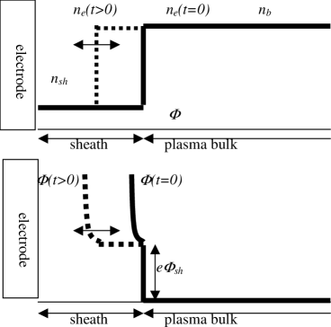
FIG. 1.: Schematic of a sheath. The negatively charged electrode pushes electrons away by different distances depending on the strength of the electric field at the electrode. Shown are the density and potential profiles at two different times. The solid line is at the time of maximum sheath expansion.

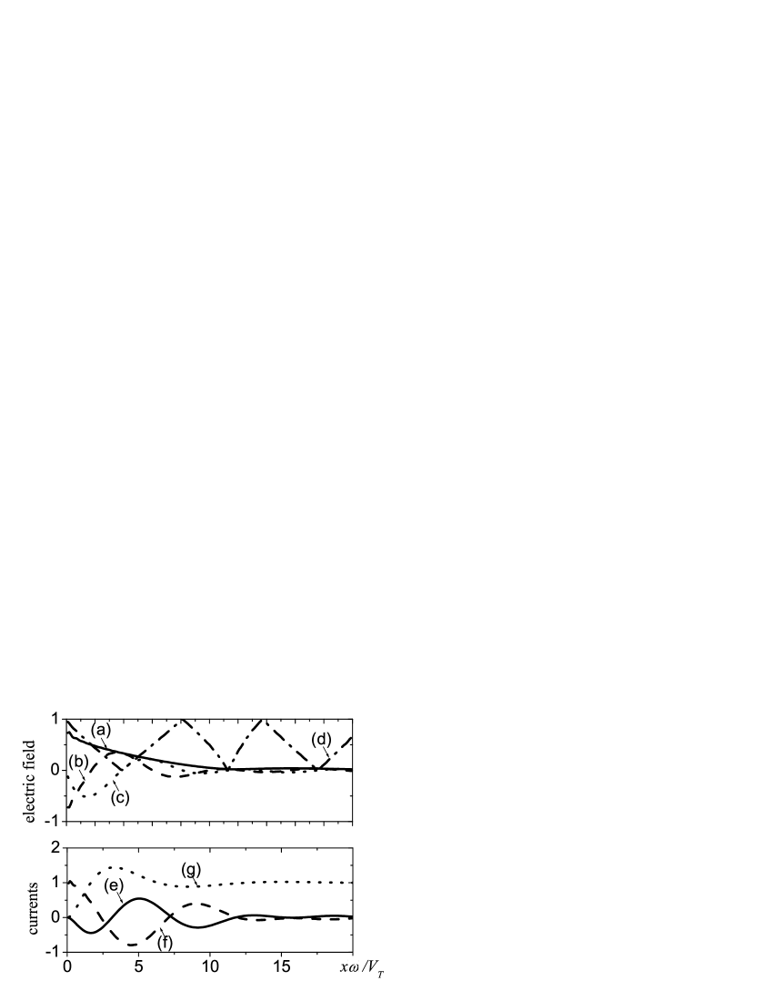
FIG. 2.: Plots of the electric field and the current normalized to their respective values in the plasma bulk, $E_{b}$ and $e^{2}nE_{b}/m\omega$, as functions of the normalized coordinate $x\omega/V_{T}$ for the following parameters: $n_{sh}/n_{b}=1/3$, $\omega/\omega_{p}=1/100$, and a Maxwellian electron distribution function. The upper graph shows profiles of $E_{1}(x)$: (a) amplitude - solid line; (b) real part - dashed line; (c) imaginary part - dotted line; and (d) phase with respect to phase of $E_{b}$ divided by $\pi$- dash-dotted line. The lower graph shows profiles of imaginary part of currents: (e) $j_{tr}$ - solid line; (f) $j_{sh}$ -dashed line; and (g) $j_{b}$ - dotted line.

FIG. 3.: Plot of the average square of the dimensionless velocity kick as a function of the dimensionless velocity for the conditions in Fig.1, taking into account (a) both $E_{1}(x)$ and $E_{b}$- solid line; (b) only $E_{b}$- dashed line; and (c) no electric field - dotted line.

FIG. 4.: Plot of the dimensionless power density as a function of the ratio of the bulk plasma density to the sheath density, taking into account (a) both $E_{1}(x)$ and $E_{b}$- solid line; (b) only $E_{b}$- dashed line; and (c) no electric field - dotted line.

REFERENCES

- [1] L.D. Landau, J. Phys. (USSR) 10, 25 (1946).
- [2] M A Lieberman, IEEE Trans. Plasma Sci. 17, 338 (1989).
- [3] M A Lieberman and V.A. Godyak, IEEE Trans. Plasma Sci. 26, 955 (1998).
- [4] I.D. Kaganovich and L.D. Tsendin, IEEE Trans. Plasma Sci. 20, 66 and 86 (1992).
- [5] T.J. Sommerer, W.N.G. Hitchon, and J.E. Lawler, Phys. Rev. Lett. 66, 2361 (1989).
- [6] M. Surendra and D. B. Graves, Phys. Rev. Lett. 66, 1469 (1991).
- [7] G. Gozadinos, M.M. Turner, and D. Vender, Phys. Rev. Lett. 87, 135004 (2001).
- [8] E.M. Lifshitz and L.P. Pitaevskii, Phisical Kinetics (Pergamon, Oxford, 1981), pp.368-376.
- [9] G.W. Hammett and F.W. Perkins Phys. Rev. Lett. 64, 3019 (1990).
- [10] F. Brunel, Phys. Rev. Lett. 59, 52 (1987).
- [11] T.-Y. B. Yang, W.L. Kruer, A.B. Langdon, and T.W. Johnston, Phys. of Plasmas 4, 2413 (1997).
- [12] K.E. Orlov, and A.S. Smirnov, Plasma Sources Sci. Technol. 8, 37 (1999).
- [13] I.D. Kaganovich, Phys. Rev. Lett. 82, 327 (1999).
- [14] Y P. Raizer, M. N. Shneider, N. A. Yatsenko. Radio-frequency capacitive discharges (Boca Raton : CRC Press, 1995).
- [15] Electrons with velocity less than may experience multiple collisions with the oscillating barrier see for example A.E. Wendt and W.N.G. Hitchon, J.Appl.Phys. 71, 4718 (1992).
- [16] Harrison, Arthur Elliot, Klystron Tubes. (1st ed. New York, McGraw-Hill Book Co., 1947).
- [17] Y.M. Aliev, I.D. Kaganovich, H. Schlüter, Phys. of Plasmas 4, 2413 (1997).
- [18] R.L. Mace, G. Amery and M.A. Hellberg, Phys. of Plasmas 6, 44 (1999).
- [19] V.A. Godyak and R.B. Piejak, Phys. Rev. Lett. 65, 996 (1990).
- [20] S.V. Berezhnoi, I.D. Kaganovich, L.D. Tsendin, Plasma Physics Reports 24 , 556 (1998).