Time series analysis for minority game simulations of financial markets

Abstract

The minority game (MG) model introduced recently provides promising insights into the understanding of the evolution of prices, indices and rates in the financial markets. In this paper we perform a time series analysis of the model employing tools from statistics, dynamical systems theory and stochastic processes. Using benchmark systems and a financial index for comparison, several conclusions are obtained about the generating mechanism for this kind of evolution. The motion is deterministic, driven by occasional random external perturbation. When the interval between two successive perturbations is sufficiently large, one can find low dimensional chaos in this regime. However, the full motion of the MG model is found to be similar to that of the first differences of the SP500 index: stochastic, nonlinear and (unit root) stationary.

, , , and

1 Introduction

The pricing of contingent claims contracts in financial economics is often based on very restrictive assumptions about the time evolution of the underlying instrument [1]. In recent years researchers have endeavored to remove some of these restrictions by proposing more realistic models which would incorporate features found in real markets [2, 3, 4, 5]. There is however a trade-off between analytic tractability and adherence to stylized facts observed from empirical financial time series. The most attractive features of the usual Black-Scholes type of models is the possibility of obtaining closed, exact formulas for the premium of derivative securities, and to build a risk free replicating strategy. Such qualities are amply used in financial institutions which require fast calculation and tools to hedge risky assets.

However, the geometric Brownian motion assumption of the Black-Scholes models ignores several empirically observed features of the real markets such as, volatility clusters, fat tails, scaling, occurrence of crashes, etc. It is as yet unknown which stochastic process is responsible for the motion of risky assets, but physicists have taken some important steps in the right direction[6, 7, 8, 4, 9]. In this work we implement a microscopic agents-based model of market dynamics which gives rise to a quite complex and rich behaviour[10] and whose output are macroscopic quantities such as price returns. By varying its parameters the model exhibits market crashes, Gaussian statistics and short ranged correlation, fat tailed returns and long range correlation. This model retains the nontrivial opinion formation structure of the grand canonical minority game[11, 12] because it incorporates two new features. The first one is to allow two categories of agents, producers (who use the market for exchanging goods), and speculators (whose aim is to profit from price fluctuations). The second feature is that speculators might choose not to trade, and in this sense the model is similar to the grand canonical ensemble of statistical physics since the number of active traders is not constant.

We perform an analysis of the time series generated by this model in order to classify its dynamical behaviour. We first test the data for unit roots and remove a simple kind of nonstationarity by taking differences wherever necessary. The BDS statistic [13], originated in the chaos literature, uses the correlation integral [14] as the basis of a test for the hypothesis that the data is independent and identically distributed (i.i.d.). We apply this statistic as a model specification test by applying it to the residue of an ARIMA, autoregressive integrated moving average, process (although this might not remove all kinds of linearity) [15]. If the null hypothesis is rejected then this is indication that the data is nonlinear. Another test based on surrogate data [16] is used to confirm the nonlinearity of the model. Since the alternative hypothesis for the BDS procedure is not specified other tests have to be applied in order to determine whether the nonlinearity comes from a stochastic or deterministic mechanism. Such distinction is subtle and here we approach this question by computing more parameters, the correlation dimension and two other procedures which do not require embeddings: recurrence plots [17, 18], and the Lempel-Ziv complexity (LZC) [19, 20]. In complement to the above procedures we implement a Bayesian approach called cluster weighted modelling (CWM) [21, 22] in order to find further indication of determinism.

The paper is organized as follows. The market model and its trajectories are analysed in Section 2. The time series analysis, including all statistical tests is discussed in Section 3. A succinct presentation of the CWM and its results are found in Section 4. Analysis of the results obtained and a classification of the model evolution are given in Section 5 while in the last section we summarize the main results and comment on future work.

2 Market Model

Inspired by the El Farol Problem proposed by Arthur [11], the so called Minority Game (MG) model introduced by Challet and Zhang [23, 12] represents a fascinating toy-model for financial market. Now it is becoming a paradigm for complex adaptive systems, in which individual members or traders repeatedly compete to be in the winning group. The game consists of $N$ agents that participate in the market buying or selling some kind of asset, e.g. stocks. At any given time agent $i$ can take two possible actions $a_{i}=\pm 1$, meaning buy or sell. Those players whose bets fall in the minority group are the winners, i.e., the sellers win if there is an excess of buyers, and vice versa. To determine the minority group we just consider the sign of the global action $A(t)=\sum_{i}a_{i}$, so that if $A(t)$ is positive the minority is the group of sellers; in this case the majority of players expect asset prices to go up.

In other words, this dynamics follows the law of demand and supply. In the end of each turn, the output is a single label, $1$ or $-1$, denoting the winning group at each time step. This output is made available to all traders, and it is the only information they can use to make decisions in subsequent turns. Indeed, they store the $m$ most recent output of winners set $\mu(t)$. In this way a limited memory of length $m$ is assigned to the traders corresponding to the most recent history bit-string that traders use to make decisions for the next step. In order to decide what action to take, agents use strategies. A strategy is an object that processes the outcomes of the winning sets in the last $m$ bets and from this information it determines whether a given agent should buy or sell for the next turn. When a tie results from the strategies, buying or selling is decided by coin tossing. The memory defines $D=2^{m}$ possible past histories so the strategy of one agent can be viewed as a D-dimensional vector, whose elements can be 1 or -1. The space $\Gamma$ of strategies is an hypercube of dimension $D$, and the total number of strategies in this space is $2^{D}$. At the beginning of the game each agent draws randomly a number $S$ of strategies from the space $\Gamma$ and keeps them forever. After each turn, the traders assigns one (virtual) point to each of the strategies which would have predicted the correct outcome. Along the game the traders always choose the strategy with the highest score. The MG is a very simple model, capable of exhibiting complex behaviour, like phase transitions between an information-efficient phase and information-inefficient phase, by just varying a control parameter $\alpha=\frac{2.2^{m}}{NS}$, e.g., the ratio between information complexity and number of strategies present in the game.

Figure 1: Figure showing the returns for (a) Minority game model with $N_{p}=1500$, $N_{s}=510$, $m=4$ and $\epsilon=0.003$ and (b) SP500 data

More realistic features are reached with the grand canonical minority game[4]. In this model we define the price process in terms of excess demand $A(t)$,

$$\log p(t+1)=\log p(t)+A(t),$$ (1)

and introduce two kinds of agents.

• The first kind is called producers, who go to the market only for the purpose of exchanging goods; they only have one strategy and in this sense they behave in a deterministic way with respect to $\mu(t)$. The number of producers is $N_{p}$.

• The other kind of agents are the speculators, who go to the market to make profit from price fluctuations. Since they are endowed with at least two strategies during the game they need to use the best strategy; in this sense speculators are adaptative agents with bounded rationality. The number of speculators is $N_{s}$.

In this version of the game, the number of speculators can change anytime, because the agent may decide not to trade in which case $a_{i}=0$. Since the strategy chosen by speculators is the one with highest score, it is very important to update the scores of each strategy at each time step. The updating of the scoring $U_{i,s}$ of each strategy $s$ belonging to agent $i$ is given by the following equations

$$U_{i,s}(t+1) = U_{i,s}(t)-a_{i,s}^{\mu(t)}A(t)\;\;\mbox{for}\;\;s>0$$

$$U_{i,0}(t+1) = U_{i,0}(t)+\epsilon$$ (2)

where $\epsilon$ is a threshold parameter. A sample of the trajectory generated by this model is shown in Fig. 1(a). An important piece of information to understand the generating mechanism of the system can be obtained from the periods where no coin is tossed. The game is necessarily deterministic during this mode of evolution and we selected a rather long period of 1114 points to perform a time series analysis in this regime.

This work is based upon the grand canonical MG model, henceforth called MG model.

3 Time Series Analysis

In this section we discuss the tools employed in time series analysis starting with the BDS statistics. We generate $10000$ points for each of the benchmark data described in the Appendix. Another benchmark is the set comprising $9998$ closing prices for the index SP500 from January 01, 1965 to January 01, 1995, shown in Fig. 1(b). All time series used here are unit root stationary with the exception of the financial index: this nonstationary is removed by taking first difference.

The BDS test uses the correlation integral [14] as the basis of a statistic to test whether a series of data is i.i.d. In the chaos literature the correlation integral is part of an efficient tool to compute the fractal dimension of objects called attractors (for a formal definition of attractor see, e.g., Ref. [24]). Given a sample of empirical data $\{x_{t}\}_{t=1}^{N}$, the theory of state-space reconstruction [25] requires that the $d$-histories of the data be constructed, where $d$ is called the embedding dimension. Under certain conditions it is possible to reproduce in this space the dynamics of the system for a correct choice of $d$. The correlation integral is a function defined on the trajectories in this space and from it one can compute the correlation dimension. A simple test for determinism consists of increasing the embedding dimension and observing the occurrence of a corresponding increase in the correlation dimension. Some conditions have to be met in order to apply this method, mainly stationarity and sufficient number of data points [26, 27, 28]. Our results show that the increase of the correlation dimension for the MG model with respect to the embedding dimension is practically identical to the stochastic benchmark series, including the index SP500. In this work we resort to better ways of analysing the occurrence of stochastic behaviour in complex time series evolution.

The BDS statistic will be applied to the residue of ARIMA processes in order to detect nonlinearity in the data. In this sense the statistic is used as a specification test. The asymptotic distribution of the statistic under the null of pure whiteness, is the standard normal distribution. The alternative hypothesis is not specified [13]. The code implemented here is taken from Ref. [29]. From Table 1, the null hypothesis for the MG model and for the SP500 index are rejected more strongly than for the nonlinear stochastic model $NLMA(2)$.

In the surrogate data analysis, a null hypothesis is tested under a measure $M$, usually some nonlinear statistic. Surrogates are copies of the original time series preserving all its linear stochastic structure. Let $M_{\mbox{orig}}$ and $M_{\mbox{surr}}$ be the test measure for the original and the surrogate data sets, respectively. The null hypothesis is rejected only if $M_{\mbox{orig}}<\langle M_{\mbox{surr}}\rangle$ or $M_{\mbox{orig}}>\langle M_{\mbox{surr}}\rangle$ for all surrogates. Some care should be taken to test the null hypothesis, otherwise false-positive rejection of null hypothesis could result. A detailed analysis on this is found in [32].

Here surrogate data sets [16, 30] are used in complement to the BDS statistic to test for nonlinearity. The null hypothesis is that the data is described by a stationary linear stochastic process with Gaussian inputs. The test statistic $M$ is a simple measure of predictability as in [31] and the procedure is to generate $19$ samples of rescaled surrogates and to compare with the MG model. If the test statistic falls outside the interval defined by the surrogates, then the null is rejected at the $95$% level. We found that, for embedding dimensions from 2 to 5, the MG is nonlinear at this level of significance, corroborating the previous result using the BDS.

In the remaining of this Section we discuss methods which do not require embeddings.

Another measure of randomness that provides further insight into time series dynamics is the Lempel-Ziv complexity [19, 20]. No embedding is necessary and the data is interpreted as a binary signal generated by some kind of source. This idea is ever present in communication theory where one wishes to determine the minimum alphabet required to code a source whose signal is to be sent through a noisy channel. Let us consider the length $L(N)$ of the minimal program that reproduces a sequence with $N$ symbols. The Lempel-Ziv algorithm is constructed by a special parsing which splits the sequence into words of the shortest length and that has not appeared previously. For example, the sequence $0011101001011011$ is parsed as $0.01.1.10.100.101.1011$. One can show that $L(N)\approx N_{w}(\log N_{w}(N)+1)$ where $N_{w}$ is the number of distinct words in a parsing and $N$ the size of the sequence. From this one can see that $L(N)$ contains a measure of randomness where a source that produces a greater number of new words is more random than a source producing a more repetitive pattern. In analogy with dynamical evolution, those systems that are composed of well defined cycles are predictable while chaotic motion and stochastic processes are always producing new kinds of trajectories that never repeat themselves. A comparison between chaos generated by differential equations and stochasticity can now be obtained. In the former case the Lempel-Ziv complexity is well below 1 while in the latter it is close to this value. More specifically, if we consider an oscillatory system such as the well known van der Pol oscillator, then $C=0.049$. For the Lorenz attractor with 2000 points $C=0.181$. In Section 5 we comment on the discrepancy between this value and that in Table 2, and discuss the use of this complexity measure in dynamical systems generated by maps. The complexity for the MG dynamics is found to be $0.82$ while the financial index has $C\approx 1$.

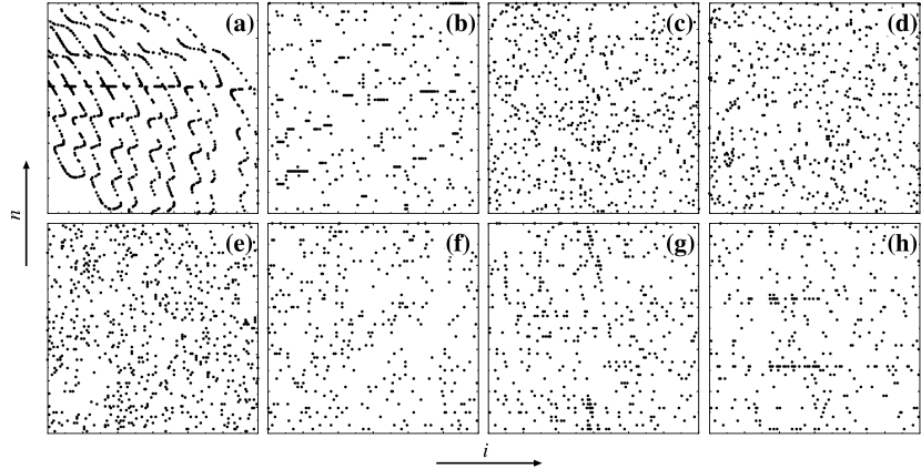
Figure 2: Recurrence plot (a) Lorenz model, (b) Henon system, (c) random numbers (d) ARMA(2,1), (e) NLMA(2), (f) SP500, (g) minority game model and (h) minority game in the deterministic regime.

The implementation of recurrence plots [17] used here is taken from [18] since it provides a clear distinction of the systems we intend to classify. The idea is to detect regions of “close returns” in a data set. The construction of the plots is simple: just compute the absolute values $\mid x_{i}-x_{n}\mid$ for all the points in the data base. If the horizontal axis is designated by $i$, corresponding to $x_{i}$, and the vertical axis by $i+n$, corresponding to $x_{i+n}$, then plot a black dot at the site $(i,n)$, whenever the absolute value difference is lower than $\delta$; otherwise plot it white. Actually the time series is normalized to $(0,1)$ and then $\delta$ is taken as $2-6$% of the average distance between successive points. The black/white pattern can be used to detect determinism in the data. There is a clear difference amongst plots generated by differential equations, maps, random data and stochastic processes as shown in Fig.  2. Patterns of horizontal segments in the recurrence plot indicate the presence of unstable periodic orbits in maps or differential equations. In this sense, these plots detect low dimensional chaos in relatively small and even noisy data sets.

4 Cluster-Weighted Modelling

An interesting probability density estimation approach to characterize and forecast time series developed by Gershenfeld, Schoner and Metois [21] is the so called cluster-weighted modelling. This seems to be a powerful technique as it characterizes extremely well the time series of nonlinear, nonstationary, non-Gaussian and discontinuous systems using probabilistic dependence of local models. The cluster-weighted modelling technique estimates the functional dependence of time series in terms of delay coordinates. The main task of this approach is to find the conditional forecast by estimating the joint probability density.

Figure 3: Fitting of data using cluster weighted analysis (a) Lorenz system, $x$ component is fitted by $\langle y|\vec{x}\rangle$ where $y=x(t)$, $\vec{x}=\{x(t-\tau),x(t-2\tau),t\}$ with delay $\tau$ and (b) minority game model, return is fitted in a similar fashion as in (a)

Let $\{y_{n},\vec{x}_{n}\}_{n=1}^{N}$ be the $N$ observations in which $\vec{x}_{n}$ are known inputs and $y_{n}$ are the corresponding outputs. By knowing the joint probability density $p(y,\vec{x})$, we can derive the conditional forecast, the expectation value of $y$ given $\vec{x}$, $\langle y|\vec{x}\rangle$. We can also deduce other quantities such as the variance of the above estimation. Actually, the joint density $p(y,\vec{x})$ is expanded terms of clusters which describe the local models. Each cluster contains three terms namely, the weight $p(c_{m})$, the domain of influence in the input space $p(\vec{x}|c_{m})$, and finally the dependence in the output space $p(y|\vec{x},c_{m})$. Thus the joint density can be written as [22],

$$p(y,\vec{x})=\sum_{m=1}^{M}p(y|\vec{x},c_{m})\,p(\vec{x}|c_{m})\,p(c_{m})$$ (3)

Once the joint density is known the other quantities can be derived from $p(y,\vec{x})$. For example, the conditional forecast is given by,

$$\langle y|\vec{x}\rangle=\int y\,p(y|\vec{x})\,dy=\frac{\sum_{m=1}^{M}f(\vec{x},\beta_{m})\,p(\vec{x}|c_{m})\,p(c_{m})}{\sum_{m=1}^{M}p(\vec{x}|c_{m})\,p(c_{m})}.$$ (4)

Here $f(\vec{x},\beta_{m})$ describes the local relationship between $\vec{x}$ and $y$. The parameters $\beta_{m}$ are found by maximizing the cluster-weighted log-likelihood. The simplest approximation for the local model is with linear coefficients of the form,

$$f(\vec{x},\beta_{m})=\sum_{i=1}^{I}\beta_{m,i}f_{i}(\vec{x}).$$ (5)

The method just described is capable of modelling a wide range of deterministic time series. Here we use cluster weighted modelling to distinguish between deterministic and stochastic time series. In deterministic systems we observe that the variances of the different clusters converge to values lower than the variance of the original time series and one can verify that this property is robust under changes of the number of clusters. On the other hand stochastic systems do not have this property. Fig. 3 illustrates the comparison between the fitting of a deterministic system (Lorenz) and the minority game data using cluster weighted modelling.

5 Analysis and Classification

The main objective is to understand the minority game mode of evolution and other similar time series behaviour. Although this system is not generated by any kind of differentiable dynamics or even stochastic differential equations, we use in its analysis methods from dynamical systems, stochastic processes and complex systems theory. Tables 1 & 2 and Fig. 2 summarize the main results. We will make frequent reference to the SP500 index since the minority game model is supposed to reproduce the dynamical evolution of financial markets and this index is used as a benchmark for comparison.

Table 1: BDS statistic

Data set	Epsilon	BDS-statistic	Decision
	($\varepsilon$)	(Embedding dimension: 2-8)
Lorenz system	0.070	610.2067, 1031.9777, 1955.1017	strongly reject
		4071.2547, 9083.3612,	linearity
		21286.7083, 51751.7514
Henon map	0.300	101.1437, 183.6664, 368.5771,	strongly reject
		716.3989, 1474.7676,	linearity
		3129.6945, 6832.0170
Random	0.500	-0.5487, -0.4410, -0.3585,	accept linearity
		-0.6511, -0.8622,
		-0.2150, 0.3504
ARMA(2,1)	0.500	-0.0270, -0.5267, -0.6978,	accept linearity
		-1.0838, -2.0321,
		-2.6126, -2.5441
NLMA(2)	0.600	6.1692, 11.6768, 13.3927,	reject linearity
		14.3183, 14.5538,
		14.8573 15.6130
SP500	0.003	15.4909, 19.8118, 23.6680,	reject linearity
		27.3441, 33.1618,
		40.8782, 50.6347
Minority Game	2.800	14.3499, 18.2687, 22.3293,	reject linearity
		26.6340, 31.2736,
		36.8712, 43.6115
Minority Game	0.03	4.8767, 5.1903, 7.3879	reject linearity
		12.3027, 19.1270,
		31.8882, 60.1133

The BDS statistic and surrogate data analysis provide clear evidence that the minority game is nonlinear. The benchmark systems described in the Appendix reproduce the expected results for the BDS in Table 2 and we can clearly see that the null hypothesis is strongly rejected for known deterministic nonlinear systems. As for the nonlinear stochastic system, the index and the MG model, the rejection occurs at all dimensions and the probability of type I error is practically zero. In particular, the BDS was used in other instances of the MG model, using different parameters and time intervals with the same result. These findings support the conclusion that there is a nonlinear mechanism in operation which drives the MG dynamics and that this property is robust to the extent tested herein.

Table 2: Summary of test results

Data set	Unit	ARIMA	BDS	LZC	Recurrence
	Root	(i,j,k)		$(C)$	plot
Lorenz system	stationary	$2,0,0$	nonlinear	0.0677	chaotic
Henon map	stationary	$4,0,3$	nonlinear	$0.5754$	chaotic
Random	stationary	$0,0,0$	linear	$\approx 1$	random
ARMA(2,1)	stationary	$2,0,0$	linear	$0.8451$	random
NLMA(2)	stationary	$0,0,2$	nonlinear	$\approx 1$	random
SP500	non-stationary	$1,0,1$	nonlinear	$\approx 1$	random
Minority Game	stationary	$1,0,5$	nonlinear	$0.82$	random
Minority Game	stationary	$1,0,0$	nonlinear	$0.6$	chaotic

The Lempel-Ziv complexity is an important parameter that can be used in the analysis of complex systems. Its advantage is that it does not require embeddings and can be easily employed in conjunction with other methods. The results in Table 1 supports the idea that there is a stochastic mechanism in operation driving the MG model. There is a higher degree of indeterminacy in the SP500 and this is perhaps due to the fact that in this index there is a certain amount of measurement noise. The surprisingly low complexity of the Lorenz system is comparable to that of limit cycles, e.g. Van der Pol oscillator. The explanation for this comes about when we compute its complexity for shorter time series. For example at 2000 points the complexity is about $2.7$ times higher than the complexity for a 10000 length series as reported in Table 2. This phenomenon does not occur for the discrete system like Henon attractor. Due to the fact that the Lorenz attractor contains a dense set of unstable periodic orbits, long time evolution affects the computation of the complexity and reveals some resemblance with periodic systems. Effects of this magnitude did not appear in the other time series analysed. In the deterministic intervals of the MG model, the complexity has a value comparable to that of the chaotic Henon map.

The Lempel-Ziv complexity, as any other test or statistic, should always be used in conjunction with other diagnostic tools. In all simulations performed so far we have never found a stochastic process with complexity less than 0.8. However there are chaotic systems with complexity beyond this value, for example the family of maps $x_{n+1}=px_{n}\,{\mbox{mod}}\,1$, $p$ a prime number. Another result is that known chaotic systems described by differential equations do not have high complexity. To conclude that a system is stochastic we employ recurrence plots and the cluster weighted modelling approach. The complexity is then used as a confirmation and, more importantly, to associate a level of stochasticity. This is done in the same way as using Lyapunov exponents to quantify chaos once determinism has been found.

The recurrence plot is a visual method which helps in the identification of similarities and differences amongst diverse modes of evolution. Several tests with differential equations and maps, represented here by the Lorenz and Henon systems, show that it is unlikely that low dimensional chaos can describe the kind of evolution found in the markets and in the MG model. In particular, recurrences are clearly identified in the Lorenz system and nothing of the kind will ever appear in stochastic models. In this sense stochastic processes are better suited to describe the financial index and the MG model. However, in the deterministic regime one can identify close return patterns similar to those of low dimensional chaotic systems.

Cluster weighted analysis reveals another aspect of the minority game behaviour. Its use in the modelling of general deterministic systems produces clusters whose variances are always smaller than the variance of the data. In contrast to this, when applied to a stochastic system the variances of the clusters are comparable to the variances of the data. Such distinction is preserved when we vary the number of clusters.

6 Conclusions and Further Work

The issue of nonstationarity is a subtle one. We limited ourselves in this study to unit root stationarity, but more sophisticated methods need to be used for the several brands of MG models and financial indices. Using the complexity parameter we found that long time evolution reveals some intrinsic features of chaotic attractors described by differential equations. Also, this parameter associated a higher complexity to the SP500 index as compared to the MG model and a possible explanation for this was given above. The recurrence plots confirm that, in general, the MG model cannot be described by low dimensional chaotic systems. The nonlinear character of the model and the index are clearly indicated by the BDS test and surrogate data analysis.

The MG model parameters employed in our simulations were chosen in the information efficient region. In the inefficient case our simulations show that the system is a non random process with complexity close to zero. The recurrence plot in this case provides a strong evidence of recurring orbits with several traces of horizontal segments. Thus, randomness is directly related to efficiency.

An important finding in our analysis of the MG game is that low dimensional chaotic regimes are possible during the evolution. This occurs for intervals of about 1000 iterations, while shorter intervals of deterministic evolution are difficult to classify. A complete study of the probabilistic structure of the deterministic phases, and their statistical significance, requires a more extensive investigation [33]. For the full motion, comprised of transitions between deterministic modes induced by random perturbations, the time series analysis has indicated the operation of a nonlinear stochastic process which is similar, but not identical, to the SP500 index. In real markets it is possible to find periods of deterministic behaviour in exchange rates for certain instruments and specific periods of time [34]. In the SP500 such occurrence is unlikely but an extensive search in the data base for several lengths and starting points is feasible. Even if deterministic modes can be found in historical stock prices, indices or rates, turning this into potential profit is a remote, but not an entirely discarded, possibility worthwhile pursuing.

Another interest in this investigation is that it provides a test amongst several models. In this sense one selects the models whose time series properties reproduce better real market evolution. In derivatives pricing a widely used test, and parameter estimation procedure, is to minimize the hedging error. This can be implemented only if a model is available, e.g. Black-Scholes. In a non-gaussian context there is no consensus on which model is appropriate. An extension of this work, which will be pursued in a future work, is to use time series methods in the several brands of agents based models and to compare them with market data. In addition to the stylized facts we should include nonlinearity, at least for the SP500, and this is an additional reason to discard simple models based on the geometric Brownian motion.

Additional investigations in this study is to model the trajectories of the Minority Game model having in view the pricing of derivatives instruments, and to use a more extensive set of statistics to examine other financial series in order to confront the similarities and differences of this model with real market data.

Appendix A Description of the data sets

The time series used as benchmarks were chosen to represent the kind of behaviour we intend to identify in the evolution of the minority game model. The Lorenz system and the Henon mapping are prototypes of deterministic behavior generated by differential equations and differentiable mappings. ARMA models and the NLMA are examples of linear and nonlinear stochastic processes. In the following we describe briefly the models used in the present study.

A.1 Lorenz system:

Nonlinear differential equations

$$\frac{dx}{dt}=\sigma(y-x);\;\;\frac{dy}{dt}=-xz+rx-y;\;\;\frac{dz}{dt}=xy-\beta z$$ (6)

The parameter values are chosen as $\sigma=16$, $\beta=4$ and $r=40$. The data series is obtained by solving Eqs. (6) numerically using fourth order Runge-Kutta method.

A.2 Henon map:

Nonlinear differentiable mapping

$$x_{t}=1-ax_{t-1}^{2}+y_{t-1};\;\;y_{t}=bx_{t-1}$$ (7)

where $a=1.4$ and $b=0.3$.

A.3 Random (Noise):

The data set is taken by drawing random points from a uniform distribution in the unit interval $x_{i}\in\text{rand}(0,1)$.

A.4 ARMA(2,1):

Linear stochastic process

$$x_{t}=0.8x_{t-1}-0.5x_{t-2}+0.4\epsilon_{t-1}+\epsilon_{t}$$ (8)

where $\epsilon_{t}\sim i.i.d.$, a normal distribution with zero mean and unit variance $N(0,1)$.

A.5 NLMA(2):

Nonlinear stochastic process

$$y_{t}=\epsilon_{t}-0.3\epsilon_{t-1}+0.2\epsilon_{t-2}+0.4\epsilon_{t-1}\epsilon_{t-2}-0.25\epsilon_{t-2}^{2}$$ (9)

where $\epsilon_{t}\sim i.i.d.$ $N(0,1)$.

References

- [1] F. Black, M. Scholes, The pricing of options and corporate liabilities, J. Polit. Econ. 81 (1973) 637–654.
- [2] N. F. Johnson, M. Hart, P. M. Hui, D. Zheng, Trader dynamics in a model market, J. Theo. App. Fin. 3 (2000) 443.
- [3] I. Giardina, J.-P. Bouchaud, M. Mezard, Microscopic models for long ranged volatility correlations, Physica A 299 (2001) 28–39.
- [4] D. Challet, M. Marsili, Y.-C. Zhang, Stylized facts of financial markets and market crashes in minority games, Physica A 294 (2001) 514–524.
- [5] T. Lux, M. Marchesi, Scaling and criticality in a stochastic multi-agent model of financial market, Nature 397 (1999) 498–500.
- [6] H. S. Stanley, R. N. Mantegna, An introduction to econophysics: correlations and complexity in finance, Cambridge University Press, Cambridge, 2000.
- [7] P. Jefferies, M. L. Hart, P. M. Hui, N. F. Johnson, From market games to real-world markets, Eur. Phys. J. B 20 (2001) 493–501.
- [8] J.-P. Bouchaud, M. Potters, Theory of financial risks: from statistical physics to risk management, Cambridge University Press, Cambridge, 2000.
- [9] J. D. Farmer, Physicists attempt to scale the ivory towers of finance, IEEE J. Comp. Sci. Eng. 1 (1999) 26–39.
- [10] D. Challet, Y. C. Zhang, On the minority game: analytical and numerical studies, Physica A 256 (1998) 514–532.
- [11] W. B. Arthur, Inductive reasoning and bounded rationality, Am. Econ. Rev. 84 (1994) 406–411.
- [12] Y.-C. Zhang, Modeling market mechanism with evolutionary games, Europhys. News 29 (1998) 51.
- [13] W. A. Brock, W. Dechert, J. Sheinkman, B. LeBaron, A test for independence based on correlation dimension, Econometric Reviews 15 (1996) 197–235.
- [14] P. Grassberger, I. Procaccia, Characterization of strange attractors, Phys. Rev. Lett 50 (1983) 346–349.
- [15] G. E. P. Box, G. M. Jenkins, G. C. Reinsel, G. Jenkins, Time series analysis for forecasing and control, 3nd ed., Holden-Day, San Francisco, 1994.
- [16] J. Theiler, S. Eubank, A. Longtin, B. Galdrikian, J. D. Farmer, Testing for nonlinearity in time-series - the method of surrogate data, Physica D 58 (1992) 77–94.
- [17] J. P. Eckmann, S. O. Kamphorst, D. Ruelle, Recurrence plots of dynamical systems, Europhys. Lett. 4 (1987) 973–977.
- [18] C. G. Gilmore, New test for chaos, J. Econ. Behav. Organ. 22 (1993) 209–237.
- [19] A. Lempel, J. Ziv, On the complexity of finite sequences, IEEE Trans. Inform. Theo. 22 (1976) 75–81.
- [20] R. Badii, A. Politi, Complexity: hierarchical strutures and scaling in physics, Cambridge University Press, Cambridge, 1999.
- [21] N. Gershenfeld, B. Schoner, E. Metois, Cluster-weighted modelling for time series analysis, Nature 397 (1999) 329–332.
- [22] N. Gershenfeld, Nature of mathematical modeling, Cambridge University Press, Cambridge, 1999.
- [23] D. Challet, Y.-C. Zhang, Emergence of cooperation and organization in an evolutionary game, Physica A 246 (1997) 407–418.
- [24] J. Milnor, On the concept of attractor, Comm. Math. Phys. 99 (1985) 177–195.
- [25] F. Takens, Detecting strange attractors in turbulence, in: D. Rand, L.-S. Young (Eds.), Dynamical systems and turbulence, Vol. 898 of Lecture notes in Mathematics, Springer-Verlag, Berlin, 1981, pp. 366–381.
- [26] T. Schreiber, Detecting and analyzing nonstationarity in a time series using nonlinear cross predictions, Phys. Rev. Lett 78 (1997) 843–846.
- [27] J. B. Gao, Recurrence time statistics for chaotic systems and their applications, Phys. Rev. Lett. 83 (1999) 3178–3181.
- [28] J. P. Eckmann, D. Ruelle, Fundamental limitations for estimating dimensions and lyapunov exponents in dynamical systems, Physica D 56 (1992) 185–187.
- [29] B. LeBaron, A fast algorithm for the bds statistics, Stud. Nonlinear Dyn. E. 2 (1997) 53–59.
- [30] R. Hegger, H. Kantz, T. Schreiber, The TISEAN software package, http://www.mpipks-dresden.mpg.de/~tisean (December 2000).
- [31] H. Kantz, T. Schreiber, Nonlinear Time Series Analysis, Cambridge University Press, Cambridge, 1997.
- [32] P. E. Rapp, C. J. Cellucci, T. A. A. Watanabe, A. M. Albano, T. I. Schmah, Surrogate data pathologies and the false-positive rejection of the null hypothesis, Int. J. Bifurcat. Chaos 11 (2001) 983–997.
- [33] F. F. Ferreira, G. Francisco, P. Muruganandam, Stochastic and deterministic structure of minority game models of financial markets, in preparation.
- [34] P. D. Grawe, H. Dewachter, M. Embrechts, Exchange Rate Theory: Chaotic Models of Foreign Exchange Markets, Blackwell Publishers, Oxford, 1993.