Optimization of a Langmuir-Taylor detector for lithium

Abstract

This paper describes the construction and optimization of a Langmuir-Taylor detector for lithium, using a rhenium ribbon. The absolute detection probability of this very sensitive detector is measured and the dependence of this probability with oxygen pressure and surface temperature is studied. Sources of background signal and their minimization are also discussed in details. And a comparison between our data concerning the response time of the detector and literature values is given. A theoretical analysis has been made: this analysis supports the validity of the Saha-Langmuir law to relate the ionization probability to the work function. Finally, the rapid variations of the work function with oxygen pressure and temperature are explained by a chemical equilibrium model.

I Introduction

Very sensitive detectors for neutral atoms, which were first necessary for Rabi experiments (see reviews in ref. king56 ; ramsey56 ), still govern the feasibility of many experiments. Two different detectors fulfill the requirements of high efficiency and low background:

• the Langmuir-Taylor detector langmuir25 ; taylor29 ; taylor30 is based on the surface ionization process. For ground state atoms, the ionization probability is large when the ionization potential is low. Therefore, this detector is mostly used with alkali atoms. For thermal atoms, the detection probability is almost independent of their velocities. The detection of a few atoms per second is feasible, if the produced ions are detected with an electron multiplier.

• the laser induced fluorescence detector, which is commonly used in cold atom experiments, has a detection probability close to $100\%$ for slow atoms. However, its detection probability decreases rapidly with the atom velocity and a large efficiency is very difficult to achieve for thermal atoms. Finally, laser stray light is usually the dominant source of background and limits the detection of a very low atomic flux.

Therefore, the Langmuir-Taylor detector is probably the best detector for thermal alkali atomic beams. Optimization of this detector is more difficult in the case of lithium, because lithium has the highest ionization potential of the alkali atoms. In the present paper, we give a detailed description of the detector in this case. More precisely, after the introduction, we describe the detector principle and its design in part 2. In part 3, we present our measurements of the detection probability, which depends on the degree of oxidation of rhenium surface persky68 ; kawano86 . The various sources of background signal and their minimization are described in part 4, while, in part 5, we discuss the detector response time. In part 6, these observations are rationalized by a theoretical modeling of the surface ionization process. Two appendices present complementary information: appendix A discusses the relation between heating current and rhenium ribbon temperature and appendix B briefly analyzes literature data concerning the dependence of rhenium work function with surface oxidation kawano86 ; kawano98 ; kawano00 ; kawano99 .

All the information needed to optimize this detector is thus collected and analyzed in the present paper. A recent paper by F. Stienkemeier et al. stienkemeier00 has described the Langmuir-Taylor detector, using a rhenium surface, applied to detect various atoms (including lithium) attached to helium droplets. Our measurements and analysis are largely complementary to those of this work.

II Detector principle and design

II.1 Detector principle

Surface ionization of an atom $A$ occurs if the ionization potential $I$ of the atom is comparable to the work function $\Phi$ of the metal. The atom is then emitted as a positive ion $A^{+}$ with a probability $P_{+}$ and as a neutral atom with the probability $(1-P_{+})$. The probability $P_{+}$ is usually assumed to be given by the Saha-Langmuir law:

$$P_{+}=\frac{1}{1+\frac{g_{0}}{g_{+}}\exp(\frac{I-\Phi}{k_{B}T})}$$ (1)

where $g_{0}$ and $g_{+}$ are the statistical weights of the ion and atom ground states (in the case of alkali atoms, $g_{0}/g_{+}=2$). The validity of this law is discussed in part 6. The wire temperature must be high, typically $1500$ K or larger, not because of its influence on the ionized fraction $P_{+}$, but to reduce the ion residence time on the surface. This residence time $\tau$ is given by:

$$\tau=\tau_{0}\exp\left(E_{ads}/k_{B}T\right)$$ (2)

Here $E_{ads}$ is the ion adsorption energy (typically a few eV) and $\tau_{0}$ should be close to the vibrational period of the ion near the surface (near $10^{-13}$ s, see table 2). Finally, the ionization probability is independent of the initial kinetic energy as long as this energy is smaller than or comparable to the adsorption energy, because the residence time on the surface is sufficient to insure thermal equilibrium with the surface.

Because of the high ionization potential of lithium, $I_{Li}=5.392$ eV, we need a metal with a large work function $\Phi$. Among refractory metals, the highest values of the work function are for platinum ($\Phi=5.77$ eV), iridium ($\Phi=5.70$ eV) kaack95 , rhenium ($\Phi=4.96$ eV) and tungsten ($\Phi=4.54$ eV) kawano99 . Moreover, oxidation increases the tungsten work function ($\Phi\approx 6$ eV following N. F. Ramsey ramsey56 , $\Phi\approx 5.9-6.2$ eV following H. Pauly and J. P. Toennies pauly68 ) and a similar effect occurs for rhenium persky68 ; kawano86 ; zandberg95 ; kawano99 . In appendix B, we discuss the dependence of rhenium work function with temperature and oxygen partial pressure: this information supports strongly the idea that rhenium is probably the best material for a lithium detector. The work function is also a function of the alkali surface coverage kaack95 ; kawano86 ; zandberg95 . This effect is very important if one uses a high flux especially when the residence time is long (i.e. at low temperature) but it is usually negligible for a high sensitivity detector dedicated to very low atomic flux.

II.2 Detector design

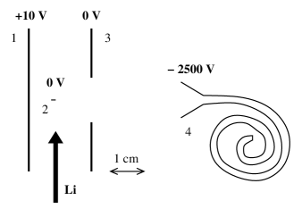
Figure 1: Schematic drawing of the detector design: 1 repeller plate; 2 endview of rhenium ribbon; 3 electrostatic lens; 4 channeltron. The arrow gives the scale and a typical choice of potentials is also indicated.

The central part of the detector is a rhenium ribbon. The ribbon thickness $a$ must be quite small, to facilitate resistive heating and cleaning (see part 4), while the width $b$ is fixed by experimental needs. For example, we use commercially available ribbons with $a=0.0008"=20.3$ $\mu m$ and $b=0.040"=1016$ $\mu m$ provided by A. D. Mackay or $a=30$ $\mu m$ and $b=760$ $\mu m$ provided by Goodfellow. The ribbon is a few centimeters long. It is heated by circulating a DC current of a few amperes, necessary to reach the operating temperature $T\simeq 1500$ K. In appendix A, we discuss the relation between the current and the ribbon temperature. Higher temperatures ($T\geq 2200$ K) are needed during the cleaning process. At $T=2000$ K, the power per unit length is about $5$ W/cm and this heat load may induce some outgassing of the vacuum tank.

The ribbon expansion goodfellow ; rembar when going from ordinary temperature to a temperature near $2000$ K is close to $1\%$. Usually, the ribbon is kept straight by a soft spring, with an applied force less than $1$ Newton (for data concerning the mechanical strength of rhenium, see ref. goodfellow ; rembar ). In our arrangement, the rhenium ribbon is spot-welded at both ends to tantalum sheets.

The ions emitted by the wire are collected and focussed on the entrance funnel of a channeltron, by a simple ion optics, as shown in figure 1. The ion trajectories have been calculated with the SIMION software SIMION and this calculation serves to define the various electrical potentials, which are further optimized by maximizing the ion signal. The repeller plate potential must not exceed a few volts, otherwise the electrons emitted by the hot wire may ionize the background gas, thus contributing to the background signal. A fast counting electronics is used to convert the channeltron pulses into a signal expressed in counts per second.

III Detection probability

The principle of our measurement is to use an effusive atomic beam of lithium. As the theory of such a beam is perfectly understood ramsey56 , we can calculate the atomic flux $dN/dt$ reaching the ribbon:

$$\frac{dN}{dt}={\mathcal{I}}\Delta\Omega$$ (3)

where the beam intensity $\mathcal{I}$ is given by ${\mathcal{I}}=n_{Li}v_{mean}a^{*}/(4\pi)$ ($n_{Li}$ is the lithium density in the oven, $v_{mean}=\sqrt{8k_{B}T/\pi m}$ is the mean velocity inside the oven, $a^{*}$ is the area of the oven exit hole) and $\Delta\Omega$ is the solid angle of the rhenium wire seen from the oven. In some experiments, we used a piezoelectric slit, whose width is tunable under vacuum, to reduce this solid angle, thus verifying the detector linearity with the atomic flux. Under these conditions, the signal remains in the linearity domain of the channeltron as long as the lithium oven temperature does not exceed $673$ K.

Several equations relating the lithium vapor pressure to the temperature appear in the literature ditchburn41 ; nesmeyanov63 . Nesmeyanov nesmeyanov63 considers that the most reliable data covering the $735-915$ K range are represented by the equation:

$$log_{10}\left(p_{Li}\right)=8.012-8172/T$$ (4)

with the pressure in Torr. We use the perfect gas approximation to convert pressure to density by $n_{Li}=p_{Li}/k_{B}T$.

Figure 2: Beam intensity $\mathcal{I}$ as a function of the oven temperature $T$. The plot presents the logarithm of $\mathcal{I}\sqrt{T}$ versus $1/T$ ($T$ in Kelvin) so that the theoretical curve deduced from equation (4) is a straight line. The triangles represent our absorption measurements, calibrated at the highest temperature using equation (4). The squares represent the same quantity deduced from the Langmuir-Taylor detector signal, assuming a $100\%$ efficiency. The absorption data prove that extrapolation of the pressure law is reasonably accurate. The Langmuir-Taylor detector signals also support the validity of the extrapolation of this pressure law. Finally, we deduce from this plot the detection probability $32\pm 5$ %.

As we must extrapolate this equation, we made a laser absorption experiment with the same atomic beam to test this extrapolation. Because of laser saturation and optical pumping, the theoretical description of laser absorption is not very simple and we use it here just as a relative measurement. The atomic density $n$ in the beam is proportional to the absorption:

$$n\propto\ln(I_{t}/I_{0})\approx(I_{0}-I_{t})/I_{0}$$

where $I_{0}$ and $I_{t}$ are the incident and transmitted laser intensities. This experiment was made in the temperature range $673-777$ K. To calibrate this measurement, we use the vapor pressure at the highest temperature of our study. The results of the absorption experiment are shown in figure 2 which plots the beam intensity $\mathcal{I}$ thus deduced. These results prove that the lithium pressure law can be safely extrapolated,for $T\geq 673$ K.

On the same figure, we have plotted the beam intensity $\mathcal{I}$ deduced from our measurements of the ion signal, as if the detection probability was equal to $100\%$. These results follow the same slope as the pressure law in this logarithmic plot, further supporting the extrapolation of the pressure law. During this experimental run, the rhenium ribbon temperature was $T=1590$ K and the residual gas pressure in the detector chamber was $3\times 10^{-8}$ mbar (corresponding to $p_{O_{2}}\approx 6\times 10^{-9}$ mbar if the residual gas is mostly air). From this plot, we get the detection probability $D_{+}=32\pm 5\%$. This error bar does not include the remaining uncertainty on the lithium vapor pressure.

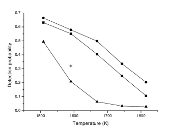
Figure 3: Measured detection probability as a function of ribbon temperature for three different oxygen pressures: dots for $p_{O2}=5.0\times 10^{-7}$ mbar, squares for $p_{O2}=2.1\times 10^{-7}$ mbar, triangles for our best vacuum ($3\times 10^{-8}$ mbar) corresponding to an estimated oxygen pressure $p_{O2}=6\times 10^{-9}$ mbar. From the saturation of these curves, we estimate that the true ionization probability is obtained by multiplying the detection probability by $1/E_{+}=1.41$ (see text). We have also represented by a cross the value of $D_{+}=32\%$ at $T=1590$ K in our best vacuum deduced from the data of figure 2.

In a second series of experiments, we measured the detection probability as a function of surface temperature and oxygen pressure: the flux of lithium atoms impinging on the rhenium ribbon was estimated to be $5.75\times 10^{5}$ atoms per second. Before each measurement, the wire was flashed at $T=2250$ K for $2$ minutes, then the heating current was adjusted to reach the working temperature and oxygen was admitted. After a stabilization period, the ion signal was measured with the lithium beam on and off and the background was substracted. We have varied the rhenium ribbon temperature in the range $1590-1880$ K. Two measurements were made by introducing oxygen with a leak valve, with oxygen pressures equal to $2.1\times 10^{-7}$ and $5.0\times 10^{-7}$ mbar (uncorrected ion gauge readings) and one measurement with our best vacuum ($3\times 10^{-8}$ mbar) corresponding to $6\times 10^{-9}$ mbar of oxygen, if the residual gas is mostly air. We thus deduce the detection probability $D_{+}$, which is plotted in figure 3. These new values of the detection probability and the first measurement ($D_{+}=32\pm 5\%$ at $T=1590$ K in our best vacuum) are not in very good agreement. This discrepancy, which illustrates the difficulty of such absolute measurements, may be due to a variation of the composition of the residual gas in the detection chamber (the experiments corresponding to figure 2 have been made one year before the experiments with a variable oxygen pressure).

$D_{+}$ is the product of the ionization probability $P_{+}$ by an ion counting efficiency $E_{+}$. This efficiency combines several experimental factors (ion collection efficiency, channeltron efficiency including electronic threshold effects) and all the errors in the estimation of the atomic flux. We have no way of measuring directly $E_{+}$, but the saturation of the detection probability with a maximum observed value $D_{+}=0.66$ must correspond to an ionization probability close to $100\%$, following literature data persky68 ; kawano86 ; kawano98 ; kawano00 ; kawano99 . From this remark, we get a good estimate of the ion counting efficiency $E_{+}=0.71$, this precise value being such that the corresponding $P_{+}$ values depend smoothly on the rhenium surface oxidized fraction $f$ defined in Appendix B. This data is analyzed in part 6.

The experiments of Stienkemeier et al. stienkemeier00 involve lithium atoms attached to helium droplets and the rhenium ribbon is kept in a higher vacuum (residual pressure $5\times 10^{-9}$ mbar) than in our experiment. The efficiency was estimated indirectly by comparison with other alkali atoms, with a peak value of $10$ % near $T=1350$ K. This value, substantially lower than our own, corresponds to a lower degree of oxidation of the rhenium surface, in agreement with the use of a higher vacuum.

IV Optimization of the background signal

The background signal has three main origins:

• the components of the background gas with ionization potentials below $9$ eV can be ionized on the rhenium surface

• a fresh rhenium wire contains a few ppm of alkali atoms. When the wire is hot, these atoms diffuse inside the wire and reach the surface where they are emitted as ions

• the background depends strongly on the oxidation of the rhenium ribbon and this can be explained by the emission of rhenium oxide ions.

We are going to discuss now these three sources of background signals. All these contributions to the background signal can be emitted from any point of the rhenium ribbon surface, but the corresponding ions are detected only if they are focused on the channeltron entrance funnel. A trick to reduce the background signal is to limit ion collection to a small part of the rhenium ribbon. In our case, the ion optics collects the ions emitted by the $5$ mm long central part of the ribbon and this length cannot be much reduced, at least for our applications.

IV.1 Ionization of the background gas

Surface ionization of many organic molecules is possible on rhenium surfaces and this technique is well established, as reviewed by Zandberg zandberg95 . The ionization probability of any component of the residual gas depends rapidly on its ionization potential $I$, through Saha-Langmuir law (1). For a species with a partial pressure close to $10^{-8}$ mbar, about $5\times 10^{11}$ molecules impinge on a $1$ centimeter length of hot wire per second. Assuming a wire temperature $T\simeq 1500K$ and an oxidized rhenium surface with $\Phi\approx 6$ eV, the corresponding contribution to the background remains below $10^{2}$ ions per second if $I-\Phi>3$ eV i.e. if $I\geq 9$ eV. Various types of organic molecules have their first ionization potential near this value and can be ionized: a mass spectrum produced by ionization of the residual gas (produced by oil diffusion pumps) on an oxidized tungsten ribbon is shown in ref. pauly68 and this spectrum is very dense. It is therefore very important to operate in a high and clean vacuum, because an oil-free vacuum contains mostly species with high ionization potentials ($H_{2}$, $H_{2}O$, $CO$…). Practically, the detector should be in a UHV chamber pumped by a turbo molecular pump or an ion getter pump. A cold trap at liquid nitrogen temperature may be useful to reduce the vapor pressure of condensable species, but its use may not be necessary.

IV.2 Cleaning the alkali content of the rhenium ribbon

Following Goodfellow goodfellow , rhenium ribbons contain $4$ ppm of potassium in mass corresponding to $3\times 10^{14}$ potassium atoms per centimeter of ribbon length. At high temperatures, these potassium atoms diffuse inside the wire, reach its surface where they are emitted as ions. Using the diffusion equation, we get the value of this ion current, assuming an homogeneous initial potassium density and a wide ribbon ($a\ll b$):

$$I_{ion}=\frac{8Nq}{\pi^{2}\tau_{1}}\sum_{p={\mbox{o}dd}}\exp\left(-\frac{p^{2}t}{\tau_{1}}\right)$$ (5)

where $N$ is the total number of potassium atoms in the ribbon and $q$ is the modulus of the electron charge. This sum of exponential is characteristic of a diffusion process, the diffusion mode of order $p$ decaying with a time constant $\tau_{p}=\tau_{1}/p^{2}$. For long times, the decay becomes purely exponential, with the time constant $\tau_{1}$ related to the diffusion constant $D$ by:

$$\tau_{1}=\frac{a^{2}}{\pi^{2}D}$$ (6)

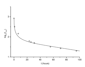
Figure 4: Ion current in picoamperes (logarithmic scale) as a function of time measured in hours (linear scale) during the baking process at a temperature $T=2250$ K. The crosses represent the measurements of the total ion current, while the curve is the best fit to this data using equation (5).

During the preparation of a ribbon made at a temperature $T=2250$ K, the repeller plate (see figure 1) served to collect about $38$ % of the emitted ions. The corresponding total ion current is plotted as a function of time in figure 4. These observations are well explained by equation (5). From the longest time constant $\tau_{1}\simeq 3.0\times 10^{5}$ s, we deduce the diffusion constant for potassium inside rhenium $D=0.3\times 10^{-15}$ $m^{2}s^{-1}$ at $T=2250$ K. As this time constant is long and as it scales like $a^{2}$, it is very important to choose a ribbon with a small thickness $a$, to minimize the duration of the cleaning process.

After $6.5$ hours of baking, we have briefly varied the wire temperature $T$ and recorded the ion current as a function of temperature. This current is proportional to the diffusion constant, thus giving the temperature dependence of the diffusion constant $D$, usually described by an Arrhenius law:

$$D=D_{0}\exp\left(-E_{diff}/k_{B}T\right)$$

From our measurements, we get the activation energy of this diffusion process, $E_{diff}=5.36\pm 0.23$ eV, and the prefactor value, $D_{0}=0.3\times 10^{-3}$ $m^{2}s^{-1}$.

IV.3 Influence of rhenium oxidation on background signal

While measuring the detection probability as a function of surface temperature and oxygen pressure, we have recorded the background signal. We discuss here only the data corresponding for $T=1508$ K, because the temperature dependence is not very simple. With our best vacuum (about $3\times 10^{-8}$ mbar), the background signal was $1-3\times 10^{3}$ counts per second and this signal increased rapidly with oxygen pressure, reaching $1.6\times 10^{4}$ and $2.6\times 10^{4}$ counts per second when the oxygen pressure was $2.1\times 10^{-7}$ or $5.0\times 10^{-7}$ mbar respectively. Moreover, the noise of this background signal is substantially larger than Poisson noise (up to $5$ times larger for $1$ second counting periods). These two effects of a strong oxidation (rapid increase of the background and excess noise) decrease considerably the performance of the detector for a small atomic flux, even if oxidation gives an important gain on detection probability.

IV.4 Operating conditions and ultimate performances

We have already explained the need for a high and clean vacuum. If one operates near $T=1500$ K, a small oxygen residual pressure of the order of a few $10^{-9}$ mbar is sufficient to reach a detection probability of the order of $10-30$ % and to keep the background at a very low level. If the initial baking time has been sufficiently long, the potassium content of the rhenium ribbon may be sufficiently reduced to give a small background signal, as long as the working temperature is not too high. In Bielefeld, where a very large set of experiments have been done loesch93 ; hobel01 , and because the background pressure, produced by an ion getter pump, is below $1\times 10^{-8}$ mbar, the typical background count rate is $100$ counts per second. In Toulouse, where we have less experience and a less good vacuum (near $3\times 10^{-8}$ mbar produced by a turbo pump), the typical background count rate is $1-3\times 10^{3}$ counts per second.

Finally, in a high vacuum, surface contamination of the rhenium ribbon by cracking of organic molecules is very slow, but it is nevertheless necessary to clean the ribbon surface from time to time by flashing it to a high temperature (typically $2250$ K) for a few minutes, to get a reproducible operation.

V Time response of the detector: residence time of lithium on a rhenium surface

The time response of a detector is very important for many applications. The dominant contribution for the present detector is the ion residence time on the surface, usually in the microsecond to millisecond range. The simplest measurement technique uses a chopped atomic beam stienkemeier00 . Another method, based on the autocorrelation function of the ion current gladyszewski94 , has also been be used and this method extends the measurement range down to the microsecond range, a value difficult to achieve by chopping atomic beams. All the data sets present in the literature have been fitted by equation (2) namely $\tau=\tau_{0}\exp\left(E_{ads}/k_{B}T\right)$.

temperature (K)	$\tau_{exp}$ ($\mu$s)	$\tau$ ($\mu$s) stienkemeier00	$\tau$ ($\mu$s) gladyszewski94
1525	215	114	82
1600	75	35	35

Table 1: Ion residence time as a function of the wire temperature. Column 1 gives the temperature deduced from the heating current (see appendix A), column 2 our measurement of the residence time, columns 3 and 4 the calculated values of $\tau$ deduced from ref. stienkemeier00 and gladyszewski94 respectively. The data collected by these authors cover the temperature range $1200-1500$ K (ref. stienkemeier00 ) and $1600-2000$ K (ref. gladyszewski94 ) so that we have to extrapolate slightly their fitted laws.

Using a chopped atomic beam, we collected two measurements, extending slightly the ranges covered by these works stienkemeier00 ; gladyszewski94 . Table 1 presents a comparison of our measurements to the values deduced from fitted laws given in these two papers. The agreement between these results is rather poor and this is easily understood for the following reasons:

• temperature measurement may be affected by systematic errors (see appendix A) and any error on the temperature has a large effect, because the residence time $\tau$ varies very rapidly with temperature

• in the simplest theoretical model (for example see ref. scheer63b ), the adsorption energy increases with the work function $\Phi$ and the work function depends on the degree of oxidation of the rhenium surface. As different experiments test rhenium surfaces with different degrees of oxidation, the different values of the residence time for the same temperature may be a real effect.

Table 2 collects the information concerning the residence time of all the alkali on rhenium, so as to illustrate the trends followed by $\tau_{0}$ and $E_{ads}$ through this chemical family. $\tau_{0}$ is expected to be close to the vibrational period of the ion near the surface and this property, well verified in several cases, is not verified by the data concerning lithium. The very long extrapolation surely explains the scatter on $\tau_{0}$ with a correlated modification of the adsorption energy (as an example, the very different parameters of ref. stienkemeier00 and gladyszewski94 for lithium lead to the same value the residence time at $T=1600$ K). The adsorption energy may also vary with surface oxidation, as discussed above, but this effect cannot explain the very large differences appearing in the case of lithium .

reference	alkali	$\tau_{0}$ in $10^{-13}$ s	$E_{ads}$ in eV
scheer63a	Cs	$1.9\pm 0.9$	$2.01\pm 0.04$
scheer63b	Rb	$0.8\pm 0.3$	$2.28\pm 0.03$
scheer63b	K	$1.0\pm 0.3$	$2.33\pm 0.03$
stienkemeier00	K	$0.01\pm 0.06$	$2.64\pm 0.06$
scheer63b	Na	$0.2\pm 0.1$	$2.75\pm 0.03$
gladyszewski94	Na	$31.$	$1.92$
stienkemeier00	Na	$0.05\pm 0.04$	$2.95\pm 0.07$
gladyszewski94	Li	$12.$	$2.37$
stienkemeier00	Li	$0.009\pm 0.006$	$3.36\pm 0.05$

Table 2: Values of the preexponential factor $\tau_{0}$ and of the adsorption energies $E_{ads}$ of the alkalis on rhenium. Column 1 gives the reference, column 2 the alkali, columns 3 and 4 the values of $\tau_{0}$ and $E_{ads}$ respectively.

VI Modeling of the surface ionization process

Surface ionization of a species $A$ is usually described using the Saha-Langmuir equation (1). This implicitly assumes a thermal equilibrium between the desorbing particle and the surface and is thus independent of the characteristics of the electron transfer process between $A$ and the surface. As will be shown below, it reproduces rather well the experimental observations. However, one can wonder about the corresponding microscopic view of the process and possible dynamical effects. The charge transfer between an atomic projectile and a free-electron metal surface is rather well understood geerlings90 and quantitative descriptions are available (see e.g. borisov96 for the alkali case). We can use this microscopic description to predict the surface ionization efficiency and compare it to the Saha-Langmuir prediction.

As an alkali atom approaches a metal surface, its electronic levels couple with the continuum of metal states, resulting in a finite lifetime of the atomic levels. The corresponding width $\Gamma$ gives the charge transfer rate between the atom and the surface. At $T=0$ K, the electron is transferred from the atom to the surface if the atomic level is above the surface Fermi level and in the opposite direction if the atomic level is below the Fermi level. For a finite temperature $T$, electron transfer occurs in both directions according to the fractional population of the metallic states at the atomic level energy position geerlings90 . For a free-electron metal, the width of the alkali level varies approximately exponentially with the distance $z$ to the surface borisov96 . Qualitatively, when an alkali leaves the surface, the very large width at small $z$ allows the alkali charge state to reach thermal equilibrium; however, this is not true at large $z$ and there exists a distance, called freezing distance, $z_{F}$, beyond which the charge state of the desorbing alkali decouples from the surface overbosch80 . Since the alkali level energy is a function $E_{a}(z)$ (for the ionic state, it roughly follows an image potential variation borisov96 ), the charge state equilibrium value changes with $z$ and the asymptotic charge state of the desorbed particle is different from its value on the surface and it a priori depends on the desorption velocity. This ’freezing distance’ discussion provides a qualitative picture of the charge transfer between a projectile and a metal surface. Quantitatively, if we assume that the desorbing particle follows a classical trajectory $z(t)$, the evolution of its charge state is governed by a rate equation geerlings90 :

$$\frac{dn_{+}}{dt} = -2\Gamma f(E_{a}(t),T)n_{+}(t)$$ (7)

$$+\Gamma\left(1-n_{+}(t)\right)\left(1-f(E_{a}(t),T)\right)$$

where $n_{+}(t)$ is the ion charge fraction, $f(E_{a}(t),T)$ the Fermi function and $E_{a}(t)$ designates $E_{a}(z(t))$.

Surface ionization is modeled by solving equation (7) for a set of different classical trajectories, representing the different possibilities for a desorbing alkali. The energies and widths in (7) are taken from the parameter-free description of the alkali free-electron metal surface study of ref. borisov96 . The initial state ($z=z_{ini}$) close to the surface is taken ionic ($n_{+}=1$) and equation (7) yields the survival probability of the ion at a large distance for each trajectory and we then have to sum the contributions from the different trajectories. In practice, we solve equation (7) up to a large $z$ distance for a set of total energies, $E$, of the desorbing particle in the ionic channel. The $z(t)$ trajectory introduced in equation (7) is common to the ionic and neutral desorption channels, which is not appropriate for large $z$. To circumvent this problem in the summation over the heavy particle energies, $E$, we assume that the charge state stabilizes around the freezing distance $z_{F}$ where we compare the local kinetic energy of the desorbing particle to the energy required for desorption in the ionic or neutral channel in order to decide whether desorption is energetically allowed or not. Ionic and neutral potential energy curves being different, this leads to a lower desorption threshold for neutral desorption. The different contributions are summed with a thermal weighting factor to yield the surface ionization probability $P_{+}$:

$$\frac{P_{+}}{1-P_{+}}=\frac{\int_{0}^{\infty}P_{s}^{+}(E)\exp\left(-E/k_{B}T\right)dE}{\int_{E_{th}}^{\infty}\left(1-P_{s}^{+}(E)\right)\exp\left(-E/k_{B}T\right)dE}$$ (8)

where $E$ is measured with respect to the ionic threshold and $E_{th}$ is equal to $E_{th}=E_{a}(\infty)-E_{a}(z_{F})$. The freezing distance, obtained from the level width calculated in ref. borisov96 , is equal to $9.6$ $a_{0}$ for lithium; it does not vary much in the energy range concerned in surface ionization.

We thus get the surface ionization probability for a given surface work function and temperature. Such an approach is indeed valid for a free-electron metal and should also be meaningful in the case of low adsorbate coverage of a metal. In the case of a low adsorbate coverage on the surface, the perturbation of the charge transfer is usually described in terms of local and non-local effects (see a review on the adsorbate effects in gauyacq98 ). The local effect is due to the local potential around the adsorbate which can strongly perturb the electron transfer in a certain region surrounding the adsorbate. The non-local effect comes from the surface work function change induced by the adsorbate. An approach like the present one only considers the non-local aspects. Local aspects are mostly visible in scattering experiments which select specific trajectories, thus probing specific areas on the surface. Surface ionization a priori concerns the entire surface and thus should average over the local effects. For very large adsorbate coverages, the electronic structure of the surface is modified, possibly leading to an insulator layer on the surface, on which the charge transfer properties are different (see e.g. a review in borisov00 ).

We are going to describe surface ionization of lithium on a rhenium surface as a function of the temperature $T$ and of the residual pressure, within the above approach and we will use the rhenium work function extracted by Kawano et al. kawano99 from their electron emission experiment (either directly the published data or the modeling of these results presented here in Appendix B). Figure 5 presents the calculated surface ionization probability of lithium for a residual air pressure of $2.0\times 10^{-7}$ Torr, compared to the experimental results of Kawano et al. kawano86 . The present microscopic results, obtained with the surface work function modeling, are seen to reproduce the experimental trends rather well, the abrupt change of the ionization probability from $100$% down to a few % as the temperature is increased clearly appears to be connected with the change of surface work function or equivalently to the degree of oxidation of the rhenium surface. The two limits (high and low $T$) in the present case correspond to either an almost clean rhenium surface and an oxidized rhenium surface. The temperature $T_{c}$ at which the abrupt change occurs depends on the residual gas pressure which directly influences the oxygen adsorption change with temperature. $T_{c}$ decreases when the residual pressure decreases. Typically, it changes by around $300$ K for a residual air pressure change between $10^{-9}$ and $2\times 10^{-6}$ Torr. The experimental and theoretical variations of the ionization probability are shifted one with respect to the other by around $40$ K. This can be due to the approximations involved in the present modeling and/or to the accuracy of the temperature scale (see below and Appendix A). Finally, the asymptotic value of the ionisation probabibility at high temperature is underestimated by our calculation and this proves that we use a too low value of the work function $\Phi_{0}$ of clean unoxidized rhenium. Clearly, this value, $\Phi_{0}=4.94$ eV, taken from our fit of Kawano et al. kawano99 data ( see Appendix B), is slightly lower than, for instance, the value obtained by Persky persky68 , $\Phi_{0}=5.0\pm 0.1$ eV.

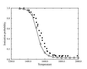
Figure 5: Ionization probability of lithium on rhenium as a function of surface temperature with an air pressure of $2\times 10^{-7}$ Torr: the full curve is the Saha-Langmuir law, using our modeling of the work function (Appendix B); the empty triangles represent the theoretical calculation described in part 6, with the same value of the work function; the dots represent the data of Kawano et al. kawano86

For surface ionization of sodium on rhenium surface, a similar agreement (not shown here) is found between the present modeling and the experimental results of Kawano et al. kawano98 . Figure 5 also presents the prediction of the Saha-Langmuir equation for the same conditions. The predictions of the present microscopic study are extremely close to those of the Saha-Langmuir equation, typically within a couple of %. In fact, this can be understood if we replace the value of $P_{s}^{+}$ from the numerical solution of equation (7) by its freezing distance approximation overbosch80 , i.e. if the final charge state $P_{s}^{+}$ is taken equal to its equilibrium value at the freezing distance:

$$P_{s}^{+}=\frac{1}{1+2\exp(\frac{E_{a}(z_{F})-\Phi}{k_{B}T})}$$ (9)

Bringing equation (9) into equation (8) then leads to the Saha-Langmuir equation (1), the value of $E_{a}(z_{F})$ disappearing from the result. One can notice that the freezing distance approximation (9) consists in applying the Saha-Langmuir law expression for the electronic levels alone at the point where the electronic levels decouple; the sum over the heavy particle energies (equation (8)), which takes into account the energy changes between $z_{F}$ and infinity, transforms it into the usual Saha-Langmuir expression for the total energy of the system evaluated at infinity. The good agreement between the present microscopic model and Saha-Langmuir expression thus proves that dynamical effects are absent and that the specificity of the metal surface-projectile charge transfer process disappears. This comforts the validity of a thermal equilibrium approach for the surface ionization process.

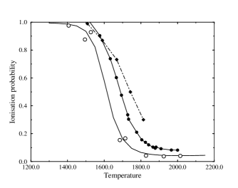
Figure 6: Ionization probability of lithium on rhenium as a function of surface temperature with an air pressure of $2\times 10^{-6}$ Torr: the full curve is the our theoretical modeling of the ionization process described in part 6, using the equations of Appendix B to describe the work function; the empty circles represent this same theoretical modeling calculation, but using directly the measurements of work function kawano99 ; the dots represent the data of Kawano et al. kawano86 and the diamonds our results (shown in figure 3) multiplied by a factor $1/E_{+}=1.41$ to get the true ionization probability.

Figure 6 presents a comparison of experimental and theoretical results for the surface ionization probability for a residual air pressure of $2.0\times 10^{-6}$ Torr. Two theoretical results are presented which were obtained either by using directly the surface work function extracted from electron emission experiments kawano99 or by using its modeling (Appendix B). The two results are close one to the other, confirming the efficiency of the modeling of the work function change. The two experimental sets are the results from reference kawano86 and the present results. The latter have been multiplied by $1.41=1/E_{+}$ to transform our detection probability result $D_{+}$ into an ionization probability $P_{+}$. Although the general behaviour of $P_{+}$ as a function of T is the same in the three sets, they appear shifted one with respect to the other. The abrupt change in $P_{+}$ as a function of T from ref. kawano86 is more rapid than in the present study. In both cases, there is an upward temperature shift when going from the model to the experiments (about $70$ K for the data of ref. kawano86 and $110$ K for our results). These differences are tentatively attributed to the accuracy of the temperature scales, both in the experimental results on surface ionization (estimated to $5$ % in the present study) and in the modeling via the use of the electron emission experimental results kawano99 .

VII Acknowledgements

We want to thank J. P. Toennies, J. P. Ziesel, A. Bordenave-Montesquieu for their help and advice and P. Echegut for information on rhenium emittance and advice on temperature measurements. We thank H. Kawano, L. Gladyszewski, F. Stienkemeier and M. Wewer for helpful correspondence. Région Midi Pyrénées is gratefully acknowledged for financial support.

Appendix A: Hot wire temperature

For a long ribbon of thickness $a$ and width $b$, the equilibrium temperature $T$ results from the equilibrium between the input power due to Joule effect and radiative losses:

$$\frac{\rho(T)I^{2}}{ab}=\epsilon(T)\sigma T^{4}[2(a+b)]$$ (10)

where $\rho(T)$ is the electrical resistivity, $\epsilon(T)$ the total emittance, both temperature dependent and $\sigma$ the Stefan-Boltzmann constant. It is a very good approximation to forget thermal conduction along the wire, as long as one does not want to describe the temperature distribution near the ribbon ends. Rhenium resistivity in $\Omega\cdot m$ rembar is well fitted by:

$$\rho(T)=26.0\times 10^{-8}\times(1+1.27\times 10^{-3}\times T)$$ (11)

for $1200<T<2000$ K. For the total emittance of rhenium, we have also fitted the three data sets collected in ref. touloukian70 and covering the range $300<T<3000$ K by a linear function of $T$:

$$\epsilon(T)=0.0852\times(1+1.15\times 10^{-3}\times T)$$ (12)

all the data points being within $\pm 20\%$ of this fit: this uncertainty produces the dominant temperature error bar equal to $5\%$. It appears from equations (11,12) that the ratio $\rho(T)/\epsilon(T)$ is a very slow function of the temperature $T$. This explains why the simple law $T\propto\sqrt{I}$ is an excellent approximation as noted by ref. stienkemeier00 . In the range $1200-2000$ K, we get:

$$T=1124\times\sqrt{I}$$ (13)

where $I$ is measured in ampere. The numerical factor $1124$ corresponds to the dimensions ($a=30$ $\mu m$ and $b=760$ $\mu m$) of the ribbon used in Toulouse and, for other ribbon geometries, this factor is easily scaled, using equation (10). All temperatures appearing in this paper were deduced from this equation (even up to $2250$ K), without recalling our estimated $5$% error bar.

We have also used an optical pyrometer to measure the temperature: the sensitivity is close $\pm 5$ Kelvin, but we have no way to test its calibration. Moreover, such pyrometers are calibrated to measure the temperature of a blackbody radiation and the readings $T_{r}$ must be corrected to take into account rhenium spectral emittance touloukian70 near $655$ nm $\epsilon_{655}\simeq 0.40$ and window transmission $\theta$. The corrected temperature $T_{c}$ is given by:

$$\frac{1}{T_{c}}=\frac{1}{T_{r}}+\frac{k_{B}}{h\nu_{655}}\ln(\epsilon_{655}\theta)$$ (14)

This correction is substantial (about $200$ K near $2000$ K). With our pyrometer, the readings $T_{r}$ are lower than the values of $T$ deduced from equation (13) by about $5\%$ while the corrected values $T_{c}$ are higher by roughly the same amount.

Appendix B: Rhenium work function $\Phi$ as a function of oxidation and temperature

The strong influence of oxidation of rhenium surface on the ionization probability of lithium was first observed by Persky persky68 in 1968. This study was continued by Kawano and coworkers kawano86 ; kawano98 ; kawano00 , who used the Saha-Langmuir law to deduce the work function from the observed ionization probability. In 1999, Kawano et al. kawano99 also measured the work function of oxidized rhenium from the emitted electron current, using the Richardson law ( $J=AT^{2}\exp\left(-\Phi/k_{B}T\right)$) to relate the current density $J$ to the work function $\Phi$. The two values of the work function differ noticeably, the work function for positive ion emission deduced from the Saha-Langmuir law being substantially larger than the work function for electron emission deduced from the Richardson law.

We first discuss the work function for electron emission because Kawano and coworkers kawano99 have collected a large data set as a function of oxygen pressure and rhenium temperature. We have developed a simple model which fits these results very satisfactorily. The oxygen surface coverage is assumed to be described by the following chemical equilibrium:

$$2\mbox{ rhenium sites }+O_{2}\rightleftharpoons 2\mbox{ oxidized rhenium sites}$$ (15)

Let $\sigma_{Re}$ and $\sigma_{ReO}$ be the density of unoxidized and oxidized sites respectively, and $p(O_{2})$ the partial pressure of molecular oxygen. The equation resulting from this chemical equilibrium is:

$$\left(\frac{\sigma_{ReO}}{\sigma_{Re}}\right)^{2}=\frac{p(O_{2})}{p_{c}(T)}$$ (16)

where $p_{c}(T)$ is the equilibrium constant of the reaction, written so as to have the dimension of a pressure. From this equation, we can deduce the fraction $f$ of the oxidized sites:

$$f=\frac{\sigma_{ReO}}{\sigma_{Re}+\sigma_{ReO}}=\frac{\sqrt{p(O_{2})/p_{c}(T)}}{1+\sqrt{p(O_{2})/p_{c}(T)}}$$ (17)

We would get a different equation if we consider that each rhenium site accepts two oxygen atoms. We have also tried to fit the data with this modified equation. As the resulting fit is considerably less good, we consider that this second hypothesis is not correct. The second assumption of the model is that the work function $\Phi$ increases linearly with the coverage $f$ from the pure metal value $\Phi_{0}$ to the completely oxidized value noted $\Phi_{0}+\Delta$:

$$\Phi=\Phi_{0}+f\Delta$$ (18)

Figure 7: Work function of rhenium as a function of air pressure in Torr (logarithmic scale) for various temperatures: diamonds for $T=1406$ K, stars for $T=1527$ K, triangles for $T=1685$ K, dots for $T=1828$ K and squares for $T=2015$ K. The experimental results are taken from figure 4 of the paper by Kawano et al. kawano99 , while the curves represent our best fit to these data, using equations (17) and (18).

This assumption is surely oversimplified but we do not see how to refine easily this model as it already represents quite well the results presented of H. Kawano et al. kawano99 in the temperature range $1400-2000$ K. Our fit to these results is presented in figure 7. Below $1400$ K, the observed variations of the work function deviate strongly from the trend observed at higher temperatures and we have not tried to fit this data. From the fits, we extract the following values: $\Phi_{0}=4.94$ eV, $\Delta=1.125$ eV and for each temperature a value of the equilibrium constant $p_{c}(T)$. The data of figure 5 of reference kawano99 are well fitted too, but with a slightly lower $\Delta$ value, $\Delta=1.00$ eV. From these fits, we have deduced 8 values of $p_{c}(T)$. A good test of the consistency of our model is that, as expected from thermodynamics, these values are well represented by the following formula:

$$log_{10}(p_{c}(T))=A+\frac{B}{T}$$ (19)

If the pressures are expressed in Torr, we get $A=9.186$ and $B=-25072$ K. The quantity $B$ corresponds to an energy $B=-2.16$ eV, which represents the energy difference between the two sides of the chemical equilibrium described by equation (15). This modeling provides a very efficient way of interpolating between the measured work function values and we used it in our treatment of the surface ionization to define the surface work function as a function of the operating conditions.

The work function of rhenium can also be deduced from the measurements of the ionization probability of sodium or lithium kawano86 ; kawano98 ; kawano00 . The analysis is somewhat more complex because the experiments were done with intense alkali halide beams and the dissociation equilibrium of the molecule on the surface must be taken into account. The Saha-Langmuir law is used to extract the work function $\Phi_{+}$ (thus noted as it differs from the electron emission value) from the data as a function of the surface temperature and oxygen pressure. However, two aspects of the analysis of Kawano and coworkers deserve further discussion:

• the ionization potential $I$ of the alkali atom is taken as a function of the wire temperature (this function appears to be $I(T)=I_{0}+2.5k_{B}T$). This is a substantial effect which is not commonly considered (see for instance ref. kaack95 , in which very accurate measurements of the platinum and iridium work function are made as a function of the temperature). Adding this unusual T dependence to the atomic ionization energy significantly contributes to the observed difference between the surface work function extracted from electron emission and the effective work function extracted from surface ionization data.

• it is surely very difficult to estimate the ionization probability to better than a few percent, in particular because the flux incident on the wire is calculated from vapor pressure data which are not very accurate (as discussed in the present paper in the lithium case). It is therefore very difficult to understand how the work function $\Phi_{+}$ can reach a value as large as $6.7$ eV (see figure 3b of ref. kawano98 where the experiment was done with NaCl): as soon as $(\Phi_{+}-I)\geq 5.3k_{B}T$, the Saha-Langmuir law predicts $P_{+}\geq 0.99$, almost impossible to distinguish experimentally from $P_{+}=1$. For temperatures close to $1500$ K, the maximum value of $\Phi_{+}$, which can be reliably deduced from Saha-Langmuir law, is not larger than $6.1$ eV when working with lithium (and only $5.8$ eV when working with sodium for which $I=5.139$ eV).

• finally, one can stress that most of the experimental results of ref. kawano86 and kawano98 on the surface ionization probability of lithium and sodium can be reproduced by Saha-Langmuir law using the surface work function extracted from electron emission kawano99 and the ionization potential of the free atom. There does not seem to be any need to introduce an effective work function for surface ionization, which could be, at best, only a parameterization of the experimental results.

Therefore, we think that the experimental results on $P_{+}$, obtained by Kawano and co-workers are very interesting for the characterisation of a surface ionization detector, but the values of $\Phi_{+}$ extracted from these should be considered with caution.

References

- (1) J. G. King and J. R. Zacharias, Advances in electronics and electron physics, vol. VIII, p 2, edited by L. Marton (Academic Press, 1956)
- (2) N. F. Ramsey, Molecular beams, (Oxford University Press, 1956)
- (3) I. Langmuir and K. H. Kingdon, Proc. Roy. Soc. A 107, 61 (1925)
- (4) J. B. Taylor, Zeits. f. Physik. 57, 242 (1929)
- (5) J. B. Taylor, Phys. Rev. 35, 375 (1930)
- (6) A. Persky, J. Chem. Phys. 50, 3835 (1969)
- (7) H. Kawano, S. Itasaka and S. Ohnishi, Int. J. Mass. Spectrom. Ion Processes, 73, 145 (1986)
- (8) E. Ya. Zandberg, Tech. Phys. 40, 865 (1995)
- (9) H. Kawano, K. Ogasawara, H. Kobayashi, A. Tanaka, T. Takahashi and Y. Tagashira, Rev. Sci. Instrum. 69, 1182 (1998)
- (10) H. Kawano, H. Mine, M. Moriyama and M. Tanigawa, Rev. Sci. Instrum. 71, 858 (2000)
- (11) H. Kawano, T. Takahashi, Y. Tagashira, H. Mine and M. Moriyama, Appl. Surf. Science 146, 105 (1999)
- (12) F. Stienkemeier, M. Wewer, F. Meier and H. O. Lutz, Rev. Scient. Instr. 71, 3480 (2000)
- (13) M. Kaack and D. Fick, Surface Science 342, 111 (1995)
- (14) H. Pauly and J. P. Toennies, Methods of experimental physics, vol. 7, Atomic interactions, p 268-275, Academic Press 1968)
- (15) Goodfellow data sheet for rhenium on the website: www.goodfellow.com
- (16) the Rembar company provides useful informations on rhenium on the website: www.rembar.com/rhen.htm
- (17) Simion 3D version 6.0 by D. A. Dahl 43rd ASMS Conference on Mass Spectrometry and Allied Topics, May 1995, Altanta, Georgia, USA, p 717
- (18) R. W. Ditchburn and J. C. Gilmour Rev. Mod. Phys. 13, 310 (1941)
- (19) A. N. Nesmeyanov, Vapor Pressure of the Elements, (Elsevier, 1963)
- (20) H.J. Loesch and F. Stienkemeier, J. Chem. Phys. 98, 9570 (1993)
- (21) O. Höbel, M.Menendez, H.J. Loesch, Phys. Chem. Chem. Phys. 3, 3633 (2001)
- (22) L. Gladyszewski, Vacuum 45, 289 (1994)
- (23) M. Scheer and J. Fine, J. Chem. Phys. 38, 307 (1963)
- (24) M. Scheer and J. Fine, J. Chem. Phys. 39, 1752 (1963)
- (25) H. Kawano and T. Kenpo, Int. J. Mass Spectrom. Ion Processes, 65, 299 (1985)
- (26) J. J. C. Geerlings and J. Los, Phys. Rep. 190, 133 (1990)
- (27) A. G. Borisov, D. Teillet-Billy, J. P. Gauyacq, H. Winter and G. Dierkes, Phys. Rev. B54, 17166 (1996)
- (28) E. G. Overbosch, B. Rasser, A. D. Tanner and J. Los, Surf. Sci. 93, 310 (1980)
- (29) A.G.Borisov and V.A.Esaulov J.Phys. Condensed Matter 12 (2000) R177
- (30) A.G. Borisov and J. P. Gauyacq, Surf. Sci. 445, 430 (2000)
- (31) J. P. Gauyacq and A. G. Borisov, J. Phys. Condensed Matter 10 6585 (1998)
- (32) Y. S. Touloukian and D. P. DeWitt, Thermophysical properties of matter, volume 7, (IFI/Plenum, 1970) pp 559-570