Magnetic Field Effects on the 1083 nm Atomic Line of Helium

Abstract

The structure of the excited $2^{3}\mathrm{S}$ and $2^{3}\mathrm{P}$ triplet states of ${}^{3}\mathrm{He}$ and ${}^{4}\mathrm{He}$ in an applied magnetic field $B$ is studied using different approximations of the atomic Hamiltonian. All optical transitions (line positions and intensities) of the 1083 nm $2^{3}\mathrm{S}$-$2^{3}\mathrm{P}$ transition are computed as a function of $B$. The effect of metastability exchange collisions between atoms in the ground state and in the $2^{3}\mathrm{S}$ metastable state is studied, and rate equations are derived, for the populations these states in the general case of an isotopic mixture in an arbitrary field $B$. It is shown that the usual spin-temperature description remains valid. A simple optical pumping model based on these rate equations is used to study the $B$-dependence of the population couplings which result from the exchange collisions. Simple spectroscopy measurements are performed using a single-frequency laser diode on the 1083 nm transition. The accuracy of frequency scans and of measurements of transition intensities is studied. Systematic experimental verifications are made for $B$=0 to 1.5 T. Optical pumping effects resulting from hyperfine decoupling in high field are observed to be in good agreement with the predictions of the simple model. Based on adequately chosen absorption measurements at 1083 nm, a general optical method to measure the nuclear polarisation of the atoms in the ground state in an arbitrary field is described. It is demonstrated at $B\sim$0.1 T, a field for which the usual optical methods could not operate.

1 Introduction

Highly polarised ${}^{3}\mathrm{He}$ is used for several applications in various domains, for instance to prepare polarised targets for nuclear physics experiments Rohe99 , to obtain spin filters for cold neutrons Becker98 ; Jones00 , or to perform magnetic resonance imaging (MRI) of air spaces in human lungs Tastevin00 ; Chupp01 . A very efficient and widely used polarisation method relies on optical pumping of the $2^{3}\mathrm{S}$ metastable state of helium with 1083 nm resonant light Colegrove63 ; Nacher85 . Transfer of nuclear polarisation to atoms in the ground state is ensured by metastability exchange collisions. Optical Pumping (OP) is usually performed in low magnetic field (up to a few mT), required only to prevent fast relaxation of the optically prepared orientation. OP can provide high nuclear polarisation, up to 80% Bigelow92 , but efficiently operates only at low pressure (of order 1 mbar) Leduc83 . Efficient production of large amounts of polarised gas is a key issue for most applications, which often require a dense gas. For instance, polarised gas must be at atmospheric pressure to be inhaled in order to perform lung MRI. Adding a neutral buffer gas after completion of OP is a simple method to increase pressure, but results in a large dilution of the polarised helium. Polarisation preserving compression of the helium gas after OP using different compressing devices is now performed by several research groups Becker94 ; Nacher99 ; Gentile00 , but it is a demanding technique and no commercial apparatus can currently be used to obtain the large compression ratio required by most applications.

Improving the efficiency of OP at higher pressure is a direct way to obtain larger magnetisation densities. Such an improvement was shown to be sufficient to perform lung MRI in humans MRIorsay . It could also facilitate subsequent mechanical compression by significantly reducing the required compression ratio and pumping speed. It was achieved by operating OP in a higher magnetic field (0.1 T) than is commonly used. High field OP in ${}^{3}\mathrm{He}$ had been previously reported at 0.1 T Flowers90 and 0.6 T Flowers97 , but the worthwhile use of high fields for OP at high pressures (tens of mbar) had not been reported until recently Courtade00 .

An important effect of a high enough magnetic field is to strongly reduce the influence of hyperfine coupling in the structures of the different excited levels of helium. In order to populate the $2^{3}\mathrm{S}$ metastable state and perform OP, a plasma discharge is sustained in the helium gas. In the various atomic and molecular excited states which are populated in the plasma, hyperfine interaction transfers nuclear orientation to electronic spin and orbital orientations. The electronic angular momentum is in turn converted into circular polarisation of the emitted light or otherwise lost during collisions. This process is actually put to use in the standard optical detection technique Bigelow92 ; Pavlovic70 in which the circular polarisation of a chosen helium spectral line emitted by the plasma is measured and the nuclear polarisation is inferred. The decoupling effect of an applied magnetic field unfortunately reduces the sensitivity of the standard optical detection method above 10 mT, and hence a different measurement technique must be used in high fields. This transfer of orientation also has an adverse effect in OP situations by inducing a net loss of nuclear polarisation in the gas. The decoupling effect of an applied field reduces this polarisation loss and may thus significantly improve the OP performance in situations of limited efficiency, such as low temperatures or high pressures. At low temperature (4.2 K), a reduced metastability exchange cross section sets a tight bottleneck and strongly limits the efficiency of OP Fitzsimmons68 ; Chapman76 ; Barb Th  ; a field increase from 1 to 40 mT was observed to provide an increase in nuclear polarisation from 17 % to 29 % in this situation NacherTh . At high gas pressures (above a few mbar) the proportion of metastable atoms is reduced and the creation of metastable molecular species is enhanced, two factors which tend to reduce the efficiency of OP ; it is not surprising that a significant improvement is obtained by suppressing relaxation channels in high field Courtade00 .

A systematic investigation of various processes relevant for OP in non-standard conditions (high field and/or high pressure) has been made, and results will be reported elsewhere CourtadeTh ; NousMolec . As mentioned earlier, an optical measurement method of nuclear polarisation in arbitrary field must be developed. It is based on absorption measurements of a probe beam, and requires a detailed knowledge of magnetic field effects on the 1083 nm transition lines. In this article we report on a detailed study of the effect of an applied magnetic field on the structure of the $2^{3}\mathrm{S}$ and $2^{3}\mathrm{P}$ atomic levels, both in ${}^{3}\mathrm{He}$ and ${}^{4}\mathrm{He}$. In the theoretical section we first present results obtained using a simple effective Hamiltonian and discuss the accuracy of computed line positions and intensities at various magnetic fields, then discuss the effect of an applied field on the metastability exchange collisions between the $2^{3}\mathrm{S}$ state and the $1^{1}\mathrm{S}_{0}$ ground state level of helium. In the experimental section we present results of measurements of the line positions and intensities up to 1.5 T, then describe an optical measurement technique of the nuclear polarisation of ${}^{3}\mathrm{He}$.

Let us finally mention that these studies have been principally motivated by OP developments, but that their results could be of interest to design or interpret experiments performed on helium atoms in the $2^{3}\mathrm{S}$ or $2^{3}\mathrm{P}$ state in an applied field, as long as metrological accuracy is not required. This includes laser cooling and Zeeman slowing Philips82 of a metastable atom beam, magnetic trapping and evaporative cooling which recently allowed two groups to obtain Bose Einstein condensation with metastable ${}^{4}\mathrm{He}$ atoms Orsay ; Paris , and similar experiments which may probe the influence of Fermi statistics with ultracold metastable ${}^{3}\mathrm{He}$ atoms.

2 Theoretical

The low-lying energy states of helium are represented in figure 1. The fine-structure splittings of the $2^{3}\mathrm{P}$ state of ${}^{4}\mathrm{He}$ and the additional effect of hyperfine interaction on splittings of the $2^{3}\mathrm{S}$ and $2^{3}\mathrm{P}$ states of ${}^{3}\mathrm{He}$ are indicated in null magnetic field.

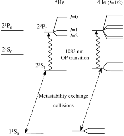
Figure 1: Ground state and first excited states of He (not to scale), showing the effects of fine and hyperfine interactions on excited level structures. The Zeeman effect is assumed negligible, except in the ground state of ${}^{3}\mathrm{He}$ in which it is grossly exaggerated to highlight the existence of two magnetic sublevels and the possibility of nuclear polarisation. Accurate values of all splittings are given in the tables in the appendix.

The ${}^{4}\mathrm{He}$ $2^{3}\mathrm{P}$ fine-structure intervals have been computed and measured with a steadily improved accuracy Storry00 ; Castillega00 , in order to provide a test of QED calculations and to measure the fine-structure constant $\alpha$. High precision isotope shift measurements of the $2^{3}\mathrm{S}$—$2^{3}\mathrm{P}$ transition of helium have also been performed to further test QED calculations and to probe the ${}^{3}\mathrm{He}$ nuclear charge radius with atomic physics experiments Shiner95 . High precision measurements and calculations of the Zeeman effect in the $2^{3}\mathrm{P}$ state of helium have also been performed Lhuillier76 ; Yang86 ; Yan94 . They were required in particular to analyse the results of fine-structure intervals measured using microwave transitions in an applied magnetic field in ${}^{4}\mathrm{He}$ Kponou81 and ${}^{3}\mathrm{He}$ Prestage85 .

All this work has produced a wealth of data which may now be used to compute the level structures and transition probabilities with a very high accuracy up to high magnetic fields (several Tesla), in spite of a small persisting disagreement between theory and experiments for the $g$-factor of the Zeeman effect in the $2^{3}\mathrm{P}$ state Yan94 ; Gonzalo97 . However, such accurate computation can be very time-consuming, especially for ${}^{3}\mathrm{He}$ in which fine-structure, hyperfine and Zeeman interaction terms of comparable importance have to be considered. A simplified approach was proposed by the Yale group Hinds85 , based on the use of an effective Hamiltonian. The hyperfine mixing of the $2^{3}\mathrm{P}$ and singlet $2^{1}\mathrm{P}$ states is the only one considered in this effective Hamiltonian, and its parameters have been experimentally determined Prestage85 . A theoretical calculation of the ${}^{3}\mathrm{He}$ $2^{3}\mathrm{P}$ structure with an accuracy of order 1 MHz later confirmed the validity of this phenomenological approach Hijikata88 . In the present article, we propose a further simplification of the effective Hamiltonian introduced by the Yale group, in which couplings to the singlet states are not explicitly considered. Instead we implicitly take into account these coupling terms, at least in part, by using the $2^{3}\mathrm{P}$ splittings measured in zero field to set the eigenvalues of the fine-structure matrices.

Results obtained using this simplified effective Hamiltonian will be compared in section 2.1.3 to those of the one including the couplings to the $2^{1}\mathrm{P}$ levels, with 3 or 6 additional magnetic sublevels, depending on the isotope. The effect of additional terms in a more elaborate form of the Zeeman Hamiltonian Yan94 than the linear approximation which we use will also be evaluated.

2.1 A simple effective Hamiltonian

2.1.1 Notations

The $1^{1}S$ ground level of helium is a singlet spin state ($S$=0), with no orbital angular momentum ($L$=0), and hence has no total electronic angular momentum ($J$=0). In ${}^{3}\mathrm{He}$, the nucleus thus carries the only angular momentum $I$, giving rise to the two magnetic sublevels $m_{I}$=$\pm 1/2$. Their relative populations, $\left(1\pm M\right)/2,$ define the nuclear polarisation $M$ of the ground state.

The level structure of ${}^{4}He$ excited states is determined from the fine-structure term and the Zeeman term in the Hamiltonian. The fine-structure term $H_{fs}$ is easily expressed in the total angular momentum representation $\left(J\right)$ using parameters given in tables 4 and 5 in the Appendix. For the Zeeman term in the applied magnetic field $B$ we shall use the simple linear form :

$$H_{Z}^{(4)}=\mu_{B}\left(g_{L}^{\prime}L+g_{S}^{\prime}S\right)\cdot B.$$ (1)

The values of Bohr magneton $\mu_{B},$ and of the orbital and spin $g$-factors $g_{L}^{\prime}$ and $g_{S}^{\prime}$ are given in table 6 in the Appendix. The situation is quite simple for the $2^{3}\mathrm{S}$ state, for which the 3 sublevels $\left|m_{S}\right\rangle$ (with $m_{S}$=$\pm 1,0$) are eigenstates at any field. For the $2^{3}\mathrm{P}$ state the Zeeman term couples sublevels of different $J$ (which however have the same $m_{J}$) and is more easily expressed in the decoupled $\left(L,S\right)$ representation. We note $\left|m_{L},m_{S}\right\rangle$ the vectors of the decoupled basis used in the $\left(L,S\right)$ representation and $\left|J;m_{J}\right\rangle$ those of the coupled basis, which are the zero-field 9 eigenstates of the $2^{3}\mathrm{P}$ state. We call $\mathrm{Z}_{1}$ to $\mathrm{Z}_{9}$ (by increasing value of the energy, see figure 2) the 9 sublevels of the $2^{3}\mathrm{P}$ state in arbitrary field. To simplify notations used in the following, we similarly call $\mathrm{Y}_{1}$ to $\mathrm{Y}_{3}$ the 3 sublevels of the $2^{3}\mathrm{S}$ state.

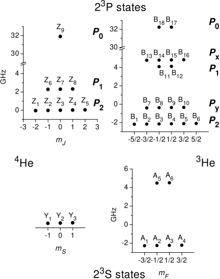
Figure 2: Left : magnetic sublevels of ${}^{4}\mathrm{He}$ in the $2^{3}\mathrm{S}$ (bottom) and $2^{3}\mathrm{P}$ (top) levels in very low magnetic field. $J$ is thus a good quantum number and $m_{J}$ is used to differentiate the atomic states. When a small field is applied, the sublevel degeneracies are removed and energies increase for increasing values of $m_{J}$ (i.e. from $Z_{1}$ to $Z_{9}$). Right : magnetic sublevels of ${}^{3}\mathrm{He}$ in very low magnetic field. $F$ and $m_{F}$ are now good quantum numbers to differentiate the atomic states. Only the $F$=3/2 $\mathrm{P}_{\mathrm{x}}$ and $\mathrm{P}_{\mathrm{y}}$ states involve a strong mixing of states of different $J$ values Nacher85 . Energies increase for increasing values of $m_{F}$ for all sublevels except in the $2^{3}\mathrm{P}_{\mathrm{0}}$ state (i.e. from $A_{1}$ to $A_{6}$ and $B_{1}$ to $B_{16}$).

The transition probabilities of all components of the 1083 nm line are evaluated using the properties of the electric dipole transition operator. For a monochromatic laser light with frequency $\omega/2\pi,$ polarisation vector $e_{\lambda},$ and intensity $I_{las}$ (expressed in W/m²), the photon absorption rate for a transition from $\mathrm{Y}_{i}$ to $\mathrm{Z}_{j}$ is given by :

$$\frac{1}{\tau_{ij}^{(4)}}=\frac{4\pi\alpha f}{m_{e}\omega\Gamma^{\prime}}~{}I_{las}~{}\frac{\left(\Gamma^{\prime}/2\right)^{2}}{\left(\Gamma^{\prime}/2\right)^{2}+\left(\omega-\omega_{ij}^{(4)}\right)^{2}}~{}T_{ij}^{(4)}(e_{\lambda}),$$ (2)

where $\alpha$ is the fine-structure constant, $f$ the oscillator strength of the $2^{3}\mathrm{S}$ -$2^{3}\mathrm{P}$ transition ($f$=0.5391 reff ; DrakeHB ), $m_{e}$ the electron mass, $\Gamma^{\prime}/2$ the total damping rate of the optical coherence between the $2^{3}\mathrm{S}$ and the $2^{3}\mathrm{P}$ states, and $T_{ij}^{(4)}(e_{\lambda})$ the transition matrix element between $\mathrm{Y}_{i}$ and $\mathrm{Z}_{j}$ Nacher85 for the light polarisation vector $e_{\lambda}$. The Lorentzian factor in equation 2 is responsible for resonant absorption (the absorption rate is decreased when the light frequency differs from the transition frequency $\omega_{ij}^{(4)}/2\pi,$ $\hbar\omega_{ij}^{(4)}$ being the energy difference between $\mathrm{Y}_{i}$ and $\mathrm{Z}_{j}$). At low enough pressure, $\Gamma^{\prime}$ is equal to the radiative decay rate $\Gamma$ of the $2^{3}\mathrm{P}$ state (the inverse of its lifetime), related to the oscillator strength $f$ by :

$$\Gamma=\frac{2\alpha\omega^{2}\hbar}{3mc^{2}}f,$$ (3)

from which $\Gamma$=1.022$\times$10⁷ s^-1 is obtained. Atomic collisions contribute to $\Gamma^{\prime}$ by a pressure-dependent amount of order 10⁸ s^-1/mbar Bloch85 . The transition matrix elements $T_{ij}^{(4)}(e_{\lambda})$ are evaluated in the $\left(L,S\right)$ representation for each of the three light polarisation states $\lambda=x\pm iy$ (circularly polarised light $\sigma_{\pm}$ propagating along the $z$-axis set by the field $B$) and $\lambda=z$ (transverse light with $\pi$ polarisation) using the selection rules given in table 7 in the Appendix. The transformation operator $P_{4}$ given in table 10 in the Appendix is used to change between the $\left(L,S\right)$ and the $\left(J\right)$ representations in the $2^{3}\mathrm{P}$ state of ${}^{4}\mathrm{He}$ and thus write a simple 9$\times$9 matrix expression for the Hamiltonian in the $\left(L,S\right)$ representation, $H_{9}$ :

$$H_{9}=P_{4}^{-1}H_{9fs}P_{4}+H_{9Z},$$ (4)

where $H_{9fs}$ is the diagonal matrix of table 4 in the Appendix and $H_{9Z}$ the diagonal matrix written from equation 1.

The level structure of ${}^{3}He$ excited states is determined from the total Hamiltonian, including hyperfine interactions. The fine-structure term $H_{fs}$ is expressed in the total angular momentum representation $\left(J\right)$ using slightly different parameters (table 5 in the Appendix) due to the small mass dependence of the fine-structure intervals. For the Zeeman term we also take into account the nuclear contribution:

$$H_{Z}^{(3)}=\mu_{B}\left(g_{L}^{\prime}L+g_{S}^{\prime}S+g_{I}I\right)\cdot B.$$ (5)

The values of all $g$-factors for ${}^{3}\mathrm{He}$ are listed in table 6 in the Appendix. For the hyperfine term, we consider the simple contact interaction between the nuclear and electronic spins and a correction term $H_{hfs}^{cor}$ :

$$H_{hfs}=A_{\mathrm{L}}I\cdot S+H_{hfs}^{cor}.$$ (6)

The matrix elements of the main contact interaction term in the decoupled $\left(S,I\right)$ representation and the values of the constants $A_{\mathrm{S}}$ and $A_{\mathrm{P}}$ for the $2^{3}\mathrm{S}$ and $2^{3}\mathrm{P}$ states are given in table 8 in the Appendix. The correction term only exists for the $2\mathrm{P}$ state Hinds85 ; Hijikata88 . When restricted to the triplet levels, it only depends on 2 parameters which are given with the matrix elements in table 11 in the Appendix.

As in the case of ${}^{4}\mathrm{He}$, we compute level structure in the decoupled representation, now $\left(L,S,I\right).$ The vectors of the decoupled bases are noted $\left|m_{S}:m_{I}\right\rangle$ for the $2^{3}\mathrm{S}$ state, and $\left|m_{L},m_{S}:m_{I}\right\rangle$ for the $2^{3}\mathrm{P}$ state. For the $2^{3}\mathrm{S}$ state, the 6$\times$6 matrix expression $H_{6}$ of the Hamiltonian is :

$$H_{6}=H_{6Z}+F_{6},$$ (7)

where $H_{6Z}$ is the diagonal matrix written from equation 5 and $F_{6}$ the matrix representation of $H_{hfs}$ (table 8 in the Appendix). For the $2^{3}\mathrm{P}$ state, the 18$\times$18 matrix $H_{18}$ is constructed  from $H_{9fs},$ $F_{6},$ $H_{hfs}^{cor}$ and $H_{Z}^{(3)}$:

$$\left\langle m_{L}^{\prime},m_{S}^{\prime}:m_{I}^{\prime}\left|H_{18}\right|m_{L},m_{S}:m_{I}\right\rangle=\\ \delta\left(m_{I}^{\prime},m_{I}\right)\left\langle m_{L}^{\prime},m_{S}^{\prime}\left|H_{9fs}\right|m_{L},m_{S}\right\rangle\\ +\delta\left(m_{L}^{\prime},m_{L}\right)\left\langle m_{S}^{\prime}:m_{I}^{\prime}\left|F_{6}\right|m_{S}:m_{I}\right\rangle\\ +\left\langle m_{L}^{\prime},m_{S}^{\prime}:m_{I}^{\prime}\left|H_{hfs}^{cor}+H_{Z}^{(3)}\right|m_{L},m_{S}:m_{I}\right\rangle.$$ (8)

The mass-dependent constants in $H_{9fs}$ and $F_{6}$ are set to the values given for ${}^{3}\mathrm{He}$ in the Appendix.

Notations similar to those of the zero-field calculation of reference Nacher85 are used. The 6 sublevels of the $2^{3}\mathrm{S}$ state are called $\mathrm{A}_{1}$ to $\mathrm{A}_{6},$ the 18 levels of the $2^{3}\mathrm{P}$ state $\mathrm{B}_{1}$ to $\mathrm{B}_{18}$ by increasing values of the energy (see figure 2). An alternative notation system, given in table 12 in the Appendix, is also used for the 6 sublevels of the $2^{3}\mathrm{S}$ state when an explicit reference to the total angular momentum projection $m_{F}$ is desired. Transition probabilities from $\mathrm{A}_{i}$ to $\mathrm{B}_{j}$ due to monochromatic light are given by a formula similar to equation 2 :

$$\frac{1}{\tau_{ij}}=\frac{4\pi\alpha f}{m_{e}\omega\Gamma^{\prime}}~{}I_{las}~{}\frac{\left(\Gamma^{\prime}/2\right)^{2}}{\left(\Gamma^{\prime}/2\right)^{2}+\left(\omega-\omega_{ij}\right)^{2}}~{}T_{ij}(e_{\lambda}),$$ (9)

in which the level energy differences $\hbar\omega_{ij}$ and the transition matrix elements $T_{ij}(e_{\lambda})$ are generalisations of the $B$=0 values computed in reference Nacher85 . To simplify notations, no upper index (3) is attached to $\tau_{ij},$ $\omega_{ij}$ and $T_{ij}$ in the case of ${}^{3}\mathrm{He}$ atoms. The small mass effect on the oscillator strength $f$ (of order 10^-4 DrakeHB ) is neglected. Sum rules on the transition matrix elements for each polarisation $e_{\lambda}$ give the relations:

$$\sum\nolimits_{i,j}T_{ij}^{(4)}\left(e_{\lambda}\right)=3,\hskip 14.22636pt\sum\nolimits_{i,j}T_{ij}\left(e_{\lambda}\right)=6.$$ (10)

In the following, the dependence of the transition matrix elements on the polarisation vector $e_{\lambda}$ will not be explicitly written. Given the selection rules described in the Appendix, the polarisation vector corresponding to a non-zero transition matrix element can be unambiguously determined.

All optical transition energies $\hbar\omega_{ij}^{(4)}$ and $\hbar\omega_{ij}$ will be referenced to $\hbar\omega_{57}(0),$ the energy of the C₁ transition in null magnetic field, which connects levels A₅ and A₆ to levels B₇ to B₁₀. Energy differences will be noted $\epsilon,$ for instance :

$$\epsilon_{ij}^{(4)}/\hbar=\omega_{ij}^{(4)}-\omega_{57}(0),~{}~{}\epsilon_{ij}/\hbar=\omega_{ij}-\omega_{57}(0).$$ (11)

They are determined from computed energy splittings in the $2^{3}\mathrm{S}$ and $2^{3}\mathrm{P}$ states of each isotope. The isotope shift contribution is adjusted to obtain the precisely measured C₉-D₂ interval (810.599 MHz, Shiner95 ).

2.1.2 Numerical Results

Numerical computation of level structure and absorption spectra in an applied field $B$ is performed in 3 steps. Matrices $H_{9}$ (for ${}^{4}\mathrm{He}$), $H_{6}$ and $H_{18}$ (for ${}^{3}\mathrm{He}$) are computed first. A standard matrix diagonalisation package (the double-precision versions of the jacobi and eigsrt routines Numrec ) is then used to compute and sort all eigenvalues (energies) and eigenvectors (components of the atomic states in the decoupled bases). All transition matrix elements $T_{ij}^{(4)}$ and $T_{ij}$ are finally evaluated, and results are output to files for further use or graphic display. Actual computation time is insignificant (e.g. 20 ms per value of $B$ on a PC using a compiled Fortran program medemander ), so that we chose not to use the matrix symmetries to reduce the matrix sizes and the computational load, in contrast with references Hinds85 ; Hijikata88 . We thus directly obtain all transitions of the 1083 nm line: 19 transitions for ${}^{4}\mathrm{He}$ (6 for $\sigma_{+}$ and for $\sigma_{-},$ 7 for $\pi$ light polarisation), and 70 transitions for ${}^{3}\mathrm{He}$ (22 for $\sigma_{+}$ and for $\sigma_{-},$ 26 for $\pi$ light polarisation). These numbers are reduced for $B$=0 to 18 for ${}^{4}\mathrm{He}$ (the $\mathrm{Y}_{2}\rightarrow\mathrm{Z}_{7},$ i.e. $\left|0\right\rangle\rightarrow\left|1;0\right\rangle$ $\pi$ transition has a null probability) and to 64 for ${}^{3}\mathrm{He}$ (the $F$=1/2$\rightarrow$ $F$=5/2 transitions, from $\mathrm{A}_{5}$ or $\mathrm{A}_{6}$ to any of $\mathrm{B}_{1}$ to $\mathrm{B}_{6}$ are forbidden by selection rules). Due to level degeneracy, the usual D₀, D₁and D₂ lines of ${}^{4}\mathrm{He,}$ and C₁ to C₉ lines of ${}^{3}\mathrm{He}$ Nacher85 are obtained for $B$=0 (figure 3, and table 9 in the Appendix).

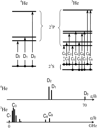
Figure 3: Top : Components of the 1083 nm line in ${}^{4}\mathrm{He}$ (left) and ${}^{3}\mathrm{He}$ (right) for $B$=0. D_J is the usual name of the transition to the $2^{3}\mathrm{P}_{J}$ level. C₁ to C₉ refer to the transitions by increasing energy. C₀ is the additional lowest energy component corresponding to a forbidden transition in zero field (see text). Bottom : positions of all the spectral lines resulting from level splittings and isotope shift. The total frequency span from C₁ to D₀ is 70.442 GHz.

An applied magnetic field removes level degeneracies (Zeeman splittings appear) and modifies the atomic states and hence the optical transition probabilities. Examples of level Zeeman energy shifts are shown in figure 4 for the $2^{3}\mathrm{S}$ state and the highest-lying $2^{3}\mathrm{P}$ levels (originating from the $2^{3}\mathrm{P}_{\mathrm{0}}$ state at low field).

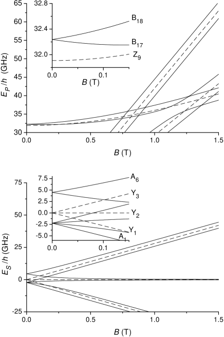
Figure 4: Level energies $E_{S}$ and $E_{P}$ of the $2^{3}\mathrm{S}$ and $2^{3}\mathrm{P}$ states are computed as a function of the applied field $B.$ They result from the fine-structure and Zeeman energy contributions for ${}^{4}\mathrm{He}$ (dashed lines),with the additional hyperfine contributions for ${}^{3}\mathrm{He}$ (solid lines). The inserts are close-ups of the low-field regions. In the $2^{3}\mathrm{P}$ state (top), only the highest lying levels are shown for simplicity.

In the $2^{3}\mathrm{S}$ state, the two Zeeman splittings are simply proportional to $B$ (28 GHz/T) for ${}^{4}\mathrm{He}$, as inferred from equation 1. For ${}^{3}\mathrm{He,}$ significant deviations from linearity occur for $\mathrm{A}_{2}$, $\mathrm{A}_{3}$ and $\mathrm{A}_{5}$ above a field of order 0.1 T, for which Zeeman shifts are significant compared to the hyperfine splitting. Level crossing of $\mathrm{A}_{4}$ and $\mathrm{A}_{5}$ (and hence interchange of names of the two states) occurs at 0.1619 T. A high-field decoupled regime is almost reached for 1.5 T (figure 4, bottom). Analytical expression for state energies and components on the decoupled $\left\{\left|m_{S}:m_{I}\right\rangle\right\}$ basis are given in the Appendix (equations 58 to A17). In the $2^{3}\mathrm{P}$ state, the situation is more complex due to fine-structure interactions and to the larger number of levels. In particular no level remains unaffected by $B$ in contrast with the situation for $\mathrm{Y}_{2}.$ As a result, $\pi$ transitions in ${}^{4}\mathrm{He}$ from $\mathrm{Y}_{2}$ to $\mathrm{Z}_{3}$ or $\mathrm{Z}_{9}$ have non-zero Zeeman frequency shifts, which are proportional to $B^{2}$ at low and moderate field although they originate from the linear Zeeman term in the Hamiltonian (equation 1). Even the $2^{3}\mathrm{P}_{\mathrm{0}}$ states, for which level mixing is weakest due to the large fine-structure gap, experience significant field effects (figure 4, top and top insert). The splitting between $\mathrm{B}_{17}$ and $\mathrm{B}_{18}$ (2.468 GHz/T at low field) is only weakly affected by the nuclear term in equation 5 ($\pm$16.2 MHz/T), and mostly results from level mixing and electronic Zeeman effects.

Examples of optical transition intensities and Zeeman frequency shifts are shown in figure 5 for ${}^{4}\mathrm{He}$ ($\pi$ light polarisation). Shifts of transition frequencies are clearly visible on the projection onto the base plane, the usual Zeeman diagram (in which no line crossing occurs). Large changes are also induced by the applied field on the transition probabilities. In particular, the forbidden D₁transition $(\mathrm{Y}_{2}\rightarrow\mathrm{Z}_{7})$ has a matrix element which linearly increases at low field ($T_{27}^{(4)}$=3.3$\times\left|B\right|$), and approaches 1 in high field (curve labelled b in figure 5). The two other strong lines at high field (2 curves labelled a superimposed in figure 5) originate from the low-field $\mathrm{Y}_{1}\rightarrow\mathrm{Z}_{2}$ and $\mathrm{Y}_{3}\rightarrow\mathrm{Z}_{8}$ transitions of D₂ and D₁ lines. All other line intensities tend to 0 at high field, in a way consistent with the sum rules of equation 10.

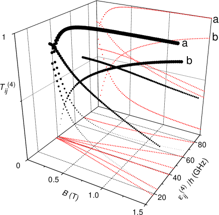
Figure 5: 3D plot of the transition matrix elements for $\pi$ light polarisation in ${}^{4}\mathrm{He,}$ $T_{ij}^{(4)}\left(\pi\right),$ (vertical axis) and of transition energy difference $\epsilon$ (with respect to C₁) as a function of $B$. To highlight the changes of the transition intensities, the symbol sizes (symbol areas) are proportional to $T_{ij}^{(4)}.$ a and b are the strongest lines in high field (see text). The projection onto the base plane is the usual Zeeman diagram.

The splittings of the C₈ and C₉ lines of ${}^{3}\mathrm{He}$ at moderate field are displayed in figure 6. Circularly polarised light, which is used in OP experiments to deposit angular momentum in the gas, is more efficiently absorbed for $\sigma_{-}$ polarisation when a field is applied. This can tentatively be related to results of our OP experiments : at $B$=0.1 T, the most efficient pumping line is actually found to be C₉, $\sigma_{-}.$ OP results at $B$=0.6 T reported in reference Flowers97 also indicate that $\sigma_{-}$ polarisation is more efficient, in spite of fluorescence measurements suggesting an imperfect polarisation of the light. One must however note that OP efficiency does not only depend on light absorption, and that level structures and metastability exchange collisions (which will be discussed below) also play a key role. Let us finally mention that the forbidden C₀ transition becomes allowed in an applied field, but that the transition probabilities remain very weak and vanish again at high field.

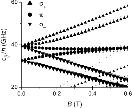
Figure 6: Plot of the Zeeman line shifts for the C₈ and C₉ lines of ${}^{3}\mathrm{He.}$ The symbol types refer to different light polarisation states. The symbol sizes (areas) are proportional to the corresponding transition matrix elements $T_{ij}$.

2.1.3 Discussion

To assess the consequences of the main approximation in our calculations, namely the restriction of the Hamiltonian to the triplet $2^{3}\mathrm{P}$ configuration, we have made a systematic comparison to the results of the full calculation including singlet-triplet mixing.

In the case of ${}^{4}\mathrm{He,}$ exact energies are of course obtained for $B$=0, and level energy differences do not exceed 1 kHz for $B$=2 T. This very good agreement results from the fact that the lowest order contribution of the singlet admixture in the $2^{3}\mathrm{P}$ state to the Zeeman effect is a third order perturbation Lhuillier76 ; Lewis70 . For similar reasons, computed transition probabilities are also almost identical, and our simple calculation is perfectly adequate for most purposes if the proper parameters of table 5 in the Appendix are used.

For ${}^{3}\mathrm{He}$ we have compared the results of the full calculation involving all 24 sublevels in the $2\mathrm{P}$ states as described by the Yale group Hinds85 and two forms of the simplified calculation restricted to the 18 sublevels of the $2^{3}\mathrm{P}$ state. The simpler form only contains the contact interaction term $A_{\mathrm{P}}I\cdot S$ in the hyperfine Hamiltonian of equation 6. The more complete calculations makes use of the full hyperfine interaction, with the correction term $H_{hfs}^{cor}$ introducing two additional parameters, $d$ and $e$.

The simpler 1-parameter calculation is similar to the zero-field calculation of reference Nacher85 (with updated values of all energy parameters), and provides a limited accuracy as shown in figure 7.

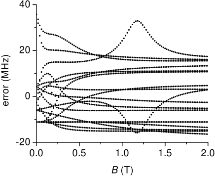
Figure 7: Errors in calculated energies for the 18 sublevels of the ${}^{3}\mathrm{He}$ $2^{3}\mathrm{P}$ state resulting from the sole use of the contact term $A_{\mathrm{P}}I\cdot S$ in the hyperfine Hamiltonian are plotted for different magnetic field intensities. Large changes of the errors occur close to level anticrossings (e.g. $m_{F}$=1/2 $\mathrm{B}_{15}$ and $\mathrm{B}_{17}$ levels close to 1.18 T, see figure 4).

Errors on the computed energies of the levels of several tens of MHz cannot be significantly reduced by adjusting $A_{\mathrm{P}}$ to a more appropriate value. This is a direct evidence that the correction term $H_{hfs}^{cor}$ unambiguously modifies the energy level diagram, with clear field-dependent signatures at moderate field and around 1 T. Errors on the transition matrix elements up to a few 10^-3 also result from neclecting $H_{hfs}^{cor}.$ Using this simple 1-parameter form of the hyperfine Hamiltonian should thus be avoided when a better accuracy is desired.

The 3-parameter calculation has also been compared to the full calculation, and a slight adjustment of parameters $A_{\mathrm{P}},$ $d$ and $e$ with respect to the corresponding parameters $C,$ $D/2$ and $E/5$ of the full calculation (which also includes the off-diagonal parameter $C^{\prime}$ Hinds85 ), now provides a more satisfactory agreement for the level energies, shown in figure 8.

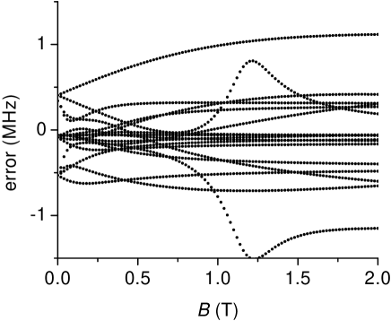
Figure 8: Errors in calculated energies for the 18 sublevels of the ${}^{3}\mathrm{He}$ $2^{3}\mathrm{P}$ state resulting from the use of the full 3-parameter hyperfine Hamiltonian are plotted for different magnetic field intensities. As in figure 7, large changes of the errors occur close to the $\mathrm{B}_{15}$ - $\mathrm{B}_{17}$ level anticrossing around 1.18 T.

Transitions matrix elements $T_{ij}$ are also obtained with good accuracy (1.3$\times$10^-4 r.m.s. difference on average for all transitions and fields, with a maximum difference of 5$\times$10^-4). The values of the 3 parameters $A_{\mathrm{P}},$ $d$ and $e$ differ by -0.019%, 3.4% and 4.6% from the corresponding parameters in the full calculation. This adjustment may effectively represent part of the off-diagonal effects in the singlet admixture, and allows to decrease the energy errors, especially below 1 T (by a factor 2-3).

The other important approximation in our calculations is related to the simplifications in the Zeeman Hamiltonian written in equations 1 and 5. The first neglected term is the non-diagonal contribution proportional to the small parameter $g_{x}$ in equation A1. The non-zero elements of this additional contribution are of order $\mu_{B}Bg_{x}/5,$ i.e. 1-2 MHz/T in frequency units. The other neglected term results from the quadratic Zeeman effect Lhuillier76 ; Yan94 ; Lewis70 , which introduces matrix elements of order $\left(\mu_{B}B\right)^{2}/R_{\infty}$ ($R_{\infty}=3.29\times 10^{6}$ GHz stands for the Rydberg constant in frequency units), i.e. 60 kHz/T². For most applications, and in particular for the experimental situations considered in the following, corrections introduced by these additional terms in the Zeeman Hamiltonian would indeed be negligible, not larger for instance than the errors in figure 8.

2.2 Metastability exchange

So far we have only addressed the effects of an applied magnetic field on the level energies and structures of the $2^{3}\mathrm{S}$ and $2^{3}\mathrm{P}$ states of helium, and the consequences for the 1083 nm optical transition. In this section we now consider the effect of the applied field on the angular momentum transfer between atoms during the so-called metastability exchange (ME) collisions, which are spin-exchange binary collisions between an atom in the ground state and one in the metastable $2^{3}\mathrm{S}$ state. They play an important role in all experimental situations where the atoms in the $2^{3}\mathrm{S}$ state are a minority species in a plasma (e.g. with a number density 10¹⁰–10¹¹ cm^-3 compared to 2.6$\times$10¹⁶ for the total density of atoms at 1 mbar in typical OP conditions). These collisions may be neglected only for experiments on atomic beams or trapped atoms for which radiative forces are used to separate the metastable atoms from the much denser gas of atoms in the ground state.

To describe the statistical properties of a mixture of ground state and $2^{3}\mathrm{S}$ state atoms we shall use a standard density operator formalism and extend the treatment introduced by Partridge and Series Partridge66 for ME collisions, later improved JDR73 ; Pinard80 and used for an OP model Nacher85 , to the case of an arbitrary magnetic field. Our first goal is to show that the “spin temperature” concept Anderson59 ; Happer72 ; Nacher85 remains valid, and that the population distribution in the $2^{3}\mathrm{S}$ state is fully determined (in the absence of OP and of relaxation) by the nuclear polarisation $M$ of the ground state. This is the result on which the optical detection method of section 3.3 relies. The second goal is to provide a formalism allowing to study the consequences of hyperfine decoupling on spin transfer during ME collisions.

2.2.1 Derivation of rate equations

We shall consider situations in which no resonance is driven between the two magnetic sublevels of the ground state of ${}^{3}\mathrm{He}$ (the ground state of ${}^{4}\mathrm{He}$ has no structure) nor between sublevels of the $2^{3}\mathrm{S}$ state. We can thus a priori assume that the density operators $\rho_{g}$ (in the ground state of ${}^{3}\mathrm{He}$), $\rho_{3}$ (in the $2^{3}\mathrm{S}$ state of  ${}^{3}\mathrm{He}$) and $\rho_{4}$ (in the $2^{3}\mathrm{S}$ state of  ${}^{4}\mathrm{He}$) are statistical mixtures of eigenstates of the Hamiltonian. The corresponding density matrices are thus diagonal and contain only populations (no coherences). With obvious notations :

$$\rho_{g} =\frac{1+M}{2}\left|+\right\rangle\left\langle+\right|+\frac{1-M}{2}\left|-\right\rangle\left\langle-\right|$$ (12)

$$\rho_{3} =\sum\nolimits_{1}^{6}a_{i}\left|\mathrm{A}_{i}\right\rangle\left\langle\mathrm{A}_{i}\right|$$ (13)

$$\rho_{4} =\sum\nolimits_{1}^{3}y_{i}\left|\mathrm{Y}_{i}\right\rangle\left\langle\mathrm{Y}_{i}\right|,$$ (14)

where $a_{i}$ and $y_{i}$ are relative populations (${\textstyle\sum}a_{i}$=${\textstyle\sum}y_{i}$=1).

An important feature of ME in helium is that in practice no depolarisation occurs during the collisions, due to the fact that all involved angular momenta are spins Pinard80 . Three kinds of ME collisions occur in an isotopic mixture, depending on the nature of the colliding atoms (${}^{3}\mathrm{He}$ or ${}^{4}\mathrm{He}$) and on their state (ground state: ${}^{3,4}\mathrm{He}$, $2^{3}\mathrm{S}$ state: ${}^{3,4}\mathrm{He}^{\mathrm{\ast}}$).

1. Following a ME collision between ${}^{3}\mathrm{He}$ atoms:

   $$\begin{array}[c]{ccccccc}{}^{3}\mathrm{He}&+&{}^{3}\mathrm{He}^{\mathrm{\ast}}&\rightarrow&{}^{3}\mathrm{He}^{\mathrm{\ast}}&+&{}^{3}\mathrm{He}\\ \rho_{g}&&\rho_{3}&&\rho_{3}^{\prime}&&\rho_{g}^{\prime}\end{array}$$

   the nuclear and electronic angular momenta are recombined in such a way that the density operators just after collision $\rho_{g}^{\prime}$ and $\rho_{3}^{\prime}$ are given by:

   $$\rho_{g}^{\prime} =\operatorname{Tr}_{e}\rho_{3}$$ (15)

   $$\rho_{3}^{\prime} =\rho_{g}\otimes\operatorname{Tr}_{n}\rho_{3}$$ (16)

   where $\operatorname{Tr}_{e},$ $\operatorname{Tr}_{n}$ are trace operators over the electronic and nuclear variables respectively JDR73 .

2. Following the collision between a  ground state ⁴He atom and a $2^{3}\mathrm{S}$ state ${}^{3}\mathrm{He}$ atom:

   $$\begin{array}[c]{ccccccc}{}^{4}\mathrm{He}&+&{}^{3}\mathrm{He}^{\mathrm{\ast}}&\rightarrow&{}^{4}\mathrm{He}^{\mathrm{\ast}}&+&{}^{3}\mathrm{He}\\ &&\rho_{3}&&\rho_{4}^{\prime\prime}&&\rho_{g}^{\prime\prime}\end{array}$$

   the density operators just after collision are:

   $$\rho_{g}^{\prime\prime} =\operatorname{Tr}_{e}\rho_{3}$$ (17)

   $$\rho_{4}^{\prime\prime} =\operatorname{Tr}_{n}\rho_{3}.$$ (18)

3. Following the collision between a$\ 2^{3}\mathrm{S}$ state ${}^{4}\mathrm{He}$ atom and a ground state ${}^{3}\mathrm{He}$ atom:

   $$\begin{array}[c]{ccccccc}{}^{3}\mathrm{He}&+&{}^{4}\mathrm{He}^{\mathrm{\ast}}&\rightarrow&{}^{3}\mathrm{He}^{\mathrm{\ast}}&+&{}^{4}\mathrm{He}\\ \rho_{g}&&\rho_{4}&&\rho_{3}^{\prime\prime\prime}&&\end{array}$$

   the density operator of the outgoing $2^{3}\mathrm{S}$ state ${}^{3}\mathrm{He}$ atom is:

   $$\rho_{3}^{\prime\prime\prime}=\rho_{g}\otimes\rho_{4}.$$ (19)

The partial trace operations in equations 15 to 18 do not introduce any coherence term in density matrices. In contrast, the tensor products in equations 16 and 19 introduce several off-diagonal terms. These are driving terms which may lead to the development of coherences in the density operators, but we shall show in the following that they can usually be neglected. Since $m_{F}$ is a good quantum number, off-diagonal terms in the tensor products only appear between 2 states of equal $m_{F}.$ With the state names defined in the Appendix (table 12), these off-diagonal terms are proportional to the operators $\left|\mathrm{A}_{+}^{h}\right\rangle\left\langle\mathrm{A}_{+}^{l}\right|$ and $\left|\mathrm{A}_{+}^{l}\right\rangle\left\langle\mathrm{A}_{+}^{h}\right|$ (for $m_{F}$=1/2), $\left|\mathrm{A}_{-}^{h}\right\rangle\left\langle\mathrm{A}_{-}^{l}\right|$ and $\left|\mathrm{A}_{-}^{l}\right\rangle\left\langle\mathrm{A}_{-}^{h}\right|$ (for $m_{F}$=-1/2). These four operators contain a similar $\sin\theta_{\pm}\cos\theta_{\pm}$ factor, where $\theta_{+}$ and $\theta_{-}$ are field-dependent level mixing parameters (see equations A14 to A17 in the Appendix). They have a time evolution characterised by a fast precessing phase, $\exp\left(i\Delta E_{\pm}t/\hbar\right),$ depending on the frequency splittings $\Delta E_{\pm}/\hbar$ of the eigenstates of equal $m_{F}.$

The time evolution of the density operators due to ME collisions is obtained from a detailed balance of the departure and arrival processes for the 3 kinds of collisions. This is similar to the method introduced by Dupont-Roc et al. JDR73 to derive a rate equation for $\rho_{g}$ and $\rho_{3}$ in pure ${}^{3}\mathrm{He}$ at low magnetic field. It is extended here to isotopic mixtures, and the effect of an arbitrary magnetic field is discussed.

The contribution of ME collisions to a rate equation for the density operator $\rho_{3}$ of the $2^{3}\mathrm{S}$ state ${}^{3}\mathrm{He}$ is obtained computing an ensemble average in the gas of the terms arising from collisions with a ${}^{3}\mathrm{He}$ atom (collision type 1, first line of the rate equation) and from collisions involving different isotopes (types 2 and 3, second line):

$$\left(\frac{d}{dt}n_{3}\rho_{3}\right)_{\mathrm{ME}}=\left\langle n_{3}N_{3}\sigma v_{33}\left(-\rho_{3}+\rho_{3}^{\prime}\right)\right\rangle\\ +\left\langle\sigma v_{34}\left(-n_{3}N_{4}\rho_{3}+n_{4}N_{3}\rho_{3}^{\prime\prime\prime}\right)\right\rangle$$ (20)

in which the brackets $\left\langle~{}\right\rangle$ correspond to the ensemble average, $N_{3,4}$ and $n_{3,4}$ are the ground state and $2^{3}\mathrm{S}$ state atom number densities of ${}^{3}\mathrm{He}$ and ${}^{4}\mathrm{He}$, $\sigma$ is the ME cross section, $v_{33}$ and $v_{34}$ are the relative velocities of colliding atoms. The ensemble averaging procedure must take into account the time evolution between collisions. For non-resonant phenomena, one is interested in steady-state situations, or in using rate equations to compute slow evolutions of the density operators (compared to the ME collision rate 1/$\tau$). For the constant or slowly varying populations ($\rho_{3},$ diagonal terms in $\rho_{3}^{\prime}$ and $\rho_{3}^{\prime\prime\prime}$), the ensemble averages simply introduce the usual thermally averaged quantities $\overline{\sigma v_{33,34}}$. For each time-dependent off-diagonal coherence, the average of the fast precessing phase involves a weighting factor $\exp(-\tilde{t}/\tau)$ to account for the distribution of times $\tilde{t}$ elapsed after a collision:

$$\left\langle\exp\left(i\Delta E_{\pm}\tilde{t}/\hbar\right)\right\rangle =\frac{1}{\tau}\int_{0}^{\infty}\exp\left(i\Delta E_{\pm}\tilde{t}/\hbar\right)\exp(-\tilde{t}/\tau)d\tilde{t}$$

$$=(1-i{}\Delta E_{\pm}\tau/\hbar)^{-1}.$$ (21)

The ME collision rate 1/$\tau$ is proportional to the helium pressure (e.g. 3.75$\times$10⁶ s^-1/mbar in pure ${}^{3}\mathrm{He}$ at room temperature JDR71 ). The splittings $\Delta E_{\pm}/\hbar$ are equal to the hyperfine splitting (6.74 GHz) in zero field, and their variation with $B$ can be derived from equations 58 and 59: $\Delta E_{+}/\hbar$ increases with $B$ while $\Delta E_{-}/\hbar$ initially decreases slightly (down to 6.35 GHz at 0.08 T), and both splittings increase linearly with $B$ at high field (with a slope of order 27.7 GHz/T). Under such conditions, $\Delta E_{\pm}\tau/\hbar$$>$1000 in a gas at 1 mbar. All coherences can thus be safely neglected in equation 20 which, when restricted to its diagonal terms, can be written as:

$$\left(\frac{d}{dt}n_{3}\rho_{3}\right)_{\mathrm{ME}}=n_{3}N_{3}\overline{\sigma v_{33}}\left(-\rho_{3}+\sum\Pi_{i}\rho_{g}\otimes\operatorname{Tr}_{n}\rho_{3}\Pi_{i}\right)\\ +\overline{\sigma v_{34}}\left(-n_{3}N_{4}\rho_{3}+n_{4}N_{3}\sum\Pi_{i}\rho_{g}\otimes\rho_{4}\Pi_{i}\right)$$ (22)

in which we note $\Pi_{i}$=$\left|\mathrm{A}_{i}\right\rangle\left\langle\mathrm{A}_{i}\right|$ the projector on the eigenstate $\mathrm{A}_{i}$.

The main differences with the result derived in JDR73 are the additional term (second line) in equation 22, which reflects the effect of ${}^{3}\mathrm{He-}^{4}\mathrm{He}$ collisions, and the replacement of the projectors on the $F$ substates by the more general projectors $\Pi_{i}$ on the eigenstates in the applied field $B$. Considering the field dependence of the frequency splittings $\Delta E_{\pm}/\hbar,$ the condition on the ME collision rate 1/$\tau$ is only slightly more stringent at 0.08 T that for $B$=0, but can be considerably relaxed at high magnetic field. The linear increase of $\Delta E_{\pm}$ and the 1/$B$ decrease of $\sin\theta_{\pm}$ (see figure 31) in the common factor of all coherences provide a $B^{2}$ increase of the acceptable collision rate, and hence of the operating pressure, for which coherences can be neglected in all density matrices, and equations 12 to 14 are valid.

The other rate equations are directly derived from equations 15, 17 and 18. Since there is no tensor product, hence no coherence source term in the relevant arrival terms, explicit ensemble averages are not required and the contribution of ME is:

$$\left(\frac{d}{dt}N_{3}\rho_{g}\right)_{\mathrm{ME}}=n_{3}N_{3}\overline{\sigma v_{33}}\left(-\rho_{g}+\operatorname{Tr}_{e}\rho_{3}\right)\\ +\overline{\sigma v_{34}}\left(-n_{4}N_{3}\rho_{g}+n_{3}N_{4}\operatorname{Tr}_{e}\rho_{3}\right)$$ (23)

$$\left(\frac{d}{dt}n_{4}\rho_{4}\right)_{\mathrm{ME}}=-n_{4}N_{3}\overline{\sigma v_{34}}\rho_{4}+n_{3}N_{4}\overline{\sigma v_{34}}\operatorname{Tr}_{n}\rho_{3}.$$ (24)

A trace operation performed on equations 22 and 24 shows that

$$\left(\frac{d}{dt}n_{4}\right)_{\mathrm{ME}}=-\left(\frac{d}{dt}n_{3}\right)_{\mathrm{ME}},$$ (25)

as expected since the three ME processes preserve the total number of atoms in the $2^{3}\mathrm{S}$ excited state.

2.2.2 Steady-state solutions

Total rate equations can be obtained by adding relaxation and OP terms to the ME terms of equations 22 and 24. They can be used to compute steady-state density matrices for the $2^{3}\mathrm{S}$ state, while the nuclear polarisation $M$ (and hence $\rho_{g}$) may have a very slow rate of change (compared to the ME collision rate 1/$\tau$). In these steady-state situations, the contribution of ME collisions to the total rate equations for the $2^{3}\mathrm{S}$ state just compensates the OP and relaxation contributions. Since the latter are traceless terms (OP and relaxation only operate population transfers between sublevels of a given isotope), by taking the trace of equation 22 or 24 one finds that the $2^{3}\mathrm{S}$ state and ground state number densities have the same isotopic ratio $R$:

$$R=n_{4}/n_{3}=N_{4}/N_{3}.$$ (26)

This results from having implicitly assumed in section 2.2.1 that all kinds of collisions have the same ME cross section. In fact destruction and excitation of of the $2^{3}\mathrm{S}$ state in the gas may differently affect ${}^{3}\mathrm{He}$ and ${}^{4}\mathrm{He}$ atoms, e.g. due to the different diffusion times to the cell walls. However in practice this has little effect compared to the very frequent ME collisions, which impose the condition of equation 26 for number densities.

To obtain simpler expressions for the rate equations, we introduce the parameters:

$$1/\tau_{e} =N_{3}\overline{\sigma v_{33}}+N_{4}\overline{\sigma v_{34}}$$ (27)

$$1/T_{e} =n_{3}\overline{\sigma v_{33}}+n_{4}\overline{\sigma v_{34}}$$ (28)

$$\mu =\overline{\sigma v_{33}}/\overline{\sigma v_{34}}$$ (29)

The rates $1/T_{e}$ and $1/\tau_{e}$ correspond to the total ME collision rate for a ${}^{3}\mathrm{He}$ atom in the ground state and in the $2^{3}\mathrm{S}$ state respectively; in steady state, equation 26 can be used to show that $\tau_{e}/T_{e}=n_{3}/N_{3}=n_{4}/N_{4}$. Since the thermal velocity distributions simply scale with the reduced masses of colliding atoms, the value of the dimensionless parameter $\mu$ can be evaluated from the energy dependence of $\sigma.$ From reference Fitzsimmons68 one can estimate $\mu\simeq$1.07 at room temperature. Rewriting equation 27 as:

$$1/\tau_{e}=\left(N_{3}+N_{4}\right)\overline{\sigma v_{33}}\frac{1+R/\mu}{1+R},$$ (30)

the ME rate in an isotopic mixture thus differs from that in pure ${}^{3}\mathrm{He}$ by at most 7 % (at large $R$) for a given total density.

Using these notations and the isotopic ratio $R$ (equation 26), the contributions of ME to rate equations become:

$$\left(\frac{d}{dt}\rho_{g}\right)_{\mathrm{ME}} =\frac{1}{T_{e}}\left(-\rho_{g}+\operatorname{Tr}_{e}\rho_{3}\right)$$ (31)

$$\left(\frac{d}{dt}\rho_{4}\right)_{\mathrm{ME}} =\frac{1}{\tau_{e}}\frac{1}{R+\mu}\left(-\rho_{4}+\operatorname{Tr}_{n}\rho_{3}\right)$$ (32)

$$\left(\frac{d}{dt}\rho_{3}\right)_{\mathrm{ME}} =\frac{1}{\tau_{e}}\left\{-\rho_{3}\right.+\frac{1}{R+\mu}\sum\Pi_{i}\times$$

$$\left.\times\left(\mu\rho_{g}\otimes\operatorname{Tr}_{n}\rho_{3}+R\rho_{g}\otimes\rho_{4}\right)\Pi_{i}\right\}.$$ (33)

In a way similar to that of reference Nacher85 we can transform equations 31 to 33 into an equivalent set of coupled rate equations for the nuclear polarisation $M$ and for the relative populations $a_{i}$ and $y_{i}$ of the $2^{3}\mathrm{S}$ states $\mathrm{A}_{i}$ and $\mathrm{Y}_{i}$:

$$\left(\frac{d}{dt}M\right)_{\mathrm{ME}} =\frac{1}{T_{e}}\left(-M+\sum_{k=1}^{6}L_{k}a_{k}\right)$$ (34)

$$\left(\frac{d}{dt}y_{i}\right)_{\mathrm{ME}} =\frac{1}{\tau_{e}}\frac{1}{R+\mu}\left(-y_{i}+\sum_{k=1}^{6}G_{ik}^{4}a_{k}\right)$$ (35)

$$\left(\frac{d}{dt}a_{i}\right)_{\mathrm{ME}} =\frac{1}{\tau_{e}}\left\{-a_{i}+\frac{1}{R+\mu}\right.\times$$

$$\times[\mu\sum_{k=1}^{6}(E_{ik}^{3} +MF_{ik}^{3})a_{k}+R\left.\sum_{k=1}^{3}(E_{ik}^{4}+MF_{ik}^{4})y_{k}]\right\}.$$ (36)

The values of the $M$-independent but $B$-dependent matrices $L,$ $G^{4},$ $E^{3},$ $F^{3},$ $E^{4}$ and $F^{4}$ are provided in the Appendix. Equation 34 directly results from computing $\operatorname{Tr}_{n}\rho_{g}I_{z}$ using equation 31. The rate equations on the relative populations are obtained by computing $\left\langle\mathrm{Y}_{i}\right|d\rho_{4}/dt\left|\mathrm{Y}_{i}\right\rangle$ using equation 32 and $\left\langle\mathrm{A}_{i}\right|d\rho_{3}/dt\left|\mathrm{A}_{i}\right\rangle$ using equation 33. The linear $M$-dependence in equation 36 directly results from that of $\rho_{g}$ (equation 12).

2.2.3 Spin temperature distributions

Anderson et al. Anderson59 have proposed that, under some conditions including fast spin exchange, the relative populations of sublevels should follow a Boltzmann-like distribution in angular momentum. This was explicitly verified for pure ${}^{3}\mathrm{He}$ in low field Nacher85 , and will now be shown for isotopic mixtures and arbitrary magnetic field. In situations where OP and relaxation processes have negligible effect on populations, the steady-state density operators are easily derived from the rate equations 31 to 33:

$$\rho_{g} =\operatorname{Tr}_{e}\rho_{3}$$ (37)

$$\rho_{4} =\operatorname{Tr}_{n}\rho_{3}$$ (38)

$$\rho_{3} =\sum\Pi_{i}\rho_{g}\otimes\operatorname{Tr}_{n}\rho_{3}\Pi_{i}.$$ (39)

Simply assuming that the populations $a_{i}$ in the $2^{3}\mathrm{S}$ state of ${}^{3}\mathrm{He}$ only depend on the $m_{F}$ values in the states $\mathrm{A}_{i},$ one can directly check using equations A14 to A17 that both $\operatorname{Tr}_{e}\rho_{3}$ (and hence equations 31 and 34) and $\operatorname{Tr}_{n}\rho_{3}$ do not depend on $B.$ Noting $e^{\beta}$ the ratio (1+$M$)/(1-$M$) of the populations in the ground state (1/$\beta$ plays the role of a spin temperature), one derives from equation 39 that the ratios of populations in the $2^{3}\mathrm{S}$ state of ${}^{3}\mathrm{He}$ are field-independent, and given by $e^{\beta\Delta m_{F}}$. These populations thus have the same distribution at all magnetic fields:

$$a_{i}=e^{\beta m_{F}}/(e^{3\beta/2}+2e^{\beta/2}+2e^{-\beta/2}+e^{-3\beta/2}).$$ (40)

Using equations 38 and A14 to A17, the populations in the $2^{3}\mathrm{S}$ state of ${}^{4}\mathrm{He}$ are in turn found to obey a similar distribution:

$$y_{i}=e^{\beta m_{S}}/(e^{\beta}+1+e^{-\beta}).$$ (41)

2.2.4 OP effects on populations

The general problem of computing all the atomic populations in arbitrary conditions is not considered in this work. It has been addressed in the low field limit using specific models in pure ${}^{3}\mathrm{He}$ Nacher85 and in isotopic mixtures Larat91 . Here we extend it to arbitrary magnetic fields, but only consider the particular situation where there is no ground state nuclear polarisation ($M$=0). It can be met in absorption spectroscopy experiments, in which a weak probing light beam may induce a deviation from the uniform population distribution imposed by $M$=0 (infinite spin temperature). We shall assume in the following that the OP process results from a depopulation mechanism in which population changes are created only by excitation of atoms from selected $2^{3}\mathrm{S}$ sublevels and not by spontaneous emission from the $2^{3}\mathrm{P}$ state (where populations are randomised by fast relaxation processes). In ${}^{3}\mathrm{He}$, this depopulation mechanism has been checked to dominate for pressures above $\sim$1 mbar Colegrove63 ; Nacher85 .

Under such conditions, and further assuming that Zeeman splittings are large enough for a single sublevel in the $2^{3}\mathrm{S}$ state to be pumped ($\mathrm{A}_{p}$ or $\mathrm{Y}_{p},$ depending on the probed isotope), the OP contribution to the time evolution of populations has a very simple form. Given the ME contribution of equation 35 or 36, the total rate equation for the pumped isotope becomes:

$$\frac{d}{dt}y_{i} =\left(\frac{d}{dt}y_{i}\right)_{\mathrm{ME}}+\frac{y_{p}}{\tau_{p}}\left(\frac{1}{3}-\delta_{\mathrm{Y}}(i,p)\right)$$ (42)

$$\text{or }~{}\frac{d}{dt}a_{i} =\left(\frac{d}{dt}a_{i}\right)_{\mathrm{ME}}+\frac{a_{p}}{\tau_{p}}\left(\frac{1}{6}-\delta_{\mathrm{A}}(i,p)\right),$$ (43)

where 1/$\tau_{p}$ is the pumping rate (equation 2 or 9) and $\delta_{\mathrm{A}}(i,p)$=1 (resp. $\delta_{\mathrm{Y}}(i,p)$=1) if the level $\mathrm{A}_{i}$ (resp. $\mathrm{Y}_{i}$) is the pumped level, 0 otherwise. In steady state, the relative populations can be obtained from the kernel of the 9$\times$9 matrix representation of the set of rate equations 35 and 43, or 36 and 42.

When a ${}^{3}\mathrm{He}$ line is probed, the ${}^{4}\mathrm{He}$ relative populations $y_{i}$ are fully imposed by ME processes only (equation 35), and can be subsituted in equation 43. The relative populations $a_{i}$ can then be obtained as the kernel of a 6$\times$6 matrix which depends on the pumped level index $p$, on the reduced pumping rate $\tau_{e}/\tau_{p}$ and on the magnetic field $B,$ but not on the isotopic ratio $R$ (as discussed at the end of the Appendix). Results showing the decrease of the pumped population $a_{p},$ and hence of the absorption of the incident light, are displayed in figure 9 as a function of $B$.

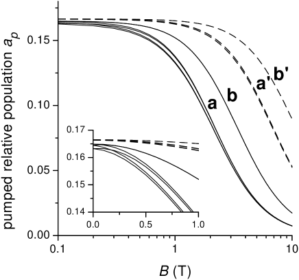
Figure 9: OP on a ${}^{3}\mathrm{He}$ level : the computed decrease of the relative population $a_{p}$ of the pumped level of ${}^{3}\mathrm{He}$ below its equilibrium value (1/6) is plotted as a function of $B$  for two values of the reduced pumping rate $\tau_{e}/\tau_{p}$ : 10^-2 (solid lines) and 10^-3 (dashed lines). For the 2 populations $a_{p}$=$a_{+}^{l}$ or $a_{-}^{h},$ the results fall on the same curve (labelled b or b^′ depending on $\tau_{e}/\tau_{p}$). For the 4 other populations, a significantly larger decrease is found (groups of curves a and a^′). The insert is an expanded view of the low-field region (with a linear $B$-scale).

A strong absorption decrease is found at high $B,$ due to larger population changes induces by OP when ME less efficiently transfers the angular momentum to the ground state (let us recall that we assume $M$=0, so that the ground state is a reservoir of infinite spin temperature). Population changes are found to be weaker for the two states $\mathrm{A}_{+}^{l}$ and $\mathrm{A}_{-}^{h}$, which both have $\left|0:\pm\right\rangle$ as the main component in high field (curves b and b^′ in figure 9).

When a ${}^{4}\mathrm{He}$ line is probed, the substitution and reduction performed above cannot be made. The full set of populations turns out to vary with the isotopic ratio $R.$ However, the OP effects are found to depend mostly on the product $R\tau_{e}/\tau_{p}$, as shown in figure 10 in the case of the state Y₃ ($m_{S}$=1). This influence of the isotopic composition extends over a wide field range, which justifies the use of isotopic mixtures to reduce the bias resulting from OP effects in our systematic quantitative measurements of ${}^{4}\mathrm{He}$ line intensities.

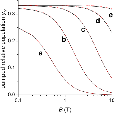
Figure 10: OP on a ${}^{4}\mathrm{He}$ level : the decrease of the ${}^{4}\mathrm{He}$ population $y_{3}$ below its equilibrium value (1/3) is plotted as a function of $B.$ The population has been computed for two values of the reduced pumping rate $\tau_{e}/\tau_{p}$ : 10^-2 (solid lines) and 10^-3 (dashed lines), and different values of $R$ (ranging from 100 to 10^-3). The population decrease mostly depends on the product $R\tau_{e}/\tau_{p}$ (10^-1,  10^-2, …10^-5 for curves a, b, … e).

Figure 11 displays a comparison of computed OP effects for the 3 sublevels of the ${}^{4}\mathrm{He}$ $2^{3}\mathrm{S}$ states. Results for the populations $y_{1}$ and $y_{3}$ are quite similar, except at large $R.$ Weaker OP effects are found for the population $y_{2},$ for which $m_{S}$=0. This feature is similar to the weaker OP effects found in ${}^{3}\mathrm{He}$ for the two states which have $m_{S}$=0, $m_{I}$=$\pm 1/2$ as main angular momenta components in high field (see figure 9).

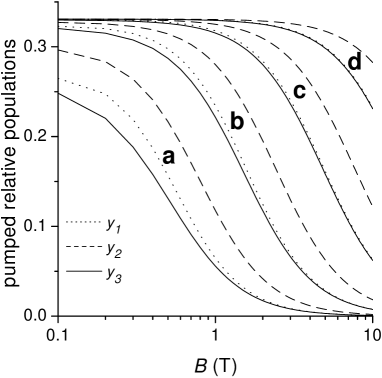
Figure 11: OP on a ${}^{4}\mathrm{He}$ level : the computed decrease of ${}^{4}\mathrm{He}$ populations $y_{1},$ $y_{2}$ and $y_{3}$ due to OP effects is plotted as a function of $B.$ The reduced pumping rate $\tau_{e}/\tau_{p}$ =10^-2 is that of the solid lines in figure 10. Four values of the isotopic ratio $R$ are used ($R\tau_{e}/\tau_{p}$ =10${}^{-2}\ \$to 10^-4 for curves a to d).

3 Experimental

In this part we present experimental results of laser absorption experiments probing the fine, hyperfine and Zeeman splittings of the 1083 nm transition in ${}^{3}\mathrm{He}$ and ${}^{4}\mathrm{He}$. Accurate microwave measurements Storry00 ; Kponou81 ; Prestage85 and high precision laser spectroscopy experiments Castillega00 ; Shiner95 ; Minardi99 ; Shiner94 are usually performed on helium atomic beams. In contrast, we have made unsophisticated absorption measurements using a single free-running laser diode on helium gas in cells at room temperature, under the usual operating conditions for nuclear polarisation of ${}^{3}\mathrm{He}$ by OP. An important consequence of these conditions is the Doppler broadening of all absorption lines. Each transition frequency $\omega_{ij}/2\pi$ (in the rest frames of the atoms) is replaced by a Gaussian distribution of width $\Delta:$

$$\Delta=\left(\omega_{ij}/2\pi\right)\sqrt{2k_{B}T/M_{at}c^{2}},$$ (44)

depending on the atomic mass $M_{at}$. At room temperature ($T$=300 K), the Doppler widths for ${}^{3}\mathrm{He}$ and ${}^{4}\mathrm{He}$ are $\Delta_{3}$=1.19 GHz and $\Delta_{4}$=1.03 GHz (the full widths at half maximum, FWHM, given by $2\Delta\sqrt{\ln 2},$ are respectively 1.98 and 1.72 GHz). The narrow Lorentzian resonant absorption profiles (with widths $\Gamma^{\prime}/2)$ in equations 2 and 9 are thus strongly modified, and broader Voigt profiles are obtained for isolated lines in standard absorption experiments. For $\Gamma^{\prime}\ll\Delta,$ these are almost Gaussian profiles of width $\Delta$. In the following, we first report on Doppler-free absorption measurements from which a good determination of frequency splittings is obtained, then on integrated absorption intensities in different magnetic fields. We finally demonstrate that absorption measurements may provide a convenient determination of the nuclear polarisation $M$.

3.1 Line positions: saturated absorption measurements

3.1.1 Experimental setup

The experiment arrangement is sketched in figure 12.

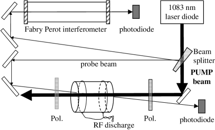
Figure 12: Main elements of a saturated absorption experiment. A magnetic field $B$ is applied either along the pump and probe beams, or perpendicular to the beams. Polarising elements (Pol.) consist of linear polarisers and/or quarter-wave plates depending on the desired polarisations of the pump and probe beams.

The helium gas samples are enclosed in sealed cylindrical Pyrex glass cells, 5 cm in diameter and 5 cm in length. Cells are filled after a careful cleaning procedure: bakeout at 700 K under high vacuum for several days, followed by 100 W RF (27 MHz) or microwave (2.4 GHz) discharges in helium with frequent gas changes until only helium lines are detected in the plasma fluorescence. Most results presented here have been recorded in cells filled with 0.53 mbar of ${}^{3}\mathrm{He}$ or helium mixture (25% ${}^{3}\mathrm{He}$, 75% ${}^{4}\mathrm{He}$). Different gas samples (from 0.2 to 30 mbar, from 10% to 100% ${}^{3}\mathrm{He}$) have also been used to study the effect of pressure and isotopic composition on the observed signals. A weak RF discharge ($<$1 W at 3 MHz) is used to populate the $2^{3}\mathrm{S}$ state in the cell during absorption measurements. The RF excitation is obtained using a pair of external electrodes. Aligning the RF electric field with $B$ provides a higher density of $2^{3}\mathrm{S}$ states and better OP results in high magnetic field.

Most data have been acquired using a specially designed air-core resistive magnet (100 mm bore diameter, with transverse optical access for 20 mm beams). In spite of a reduced footprint (30$\times$20 cm², axis height 15 cm) which conveniently permits installation on an optical table, this magnet provides a fair homogeneity. The computed relative inhomogeneity is $<$10^-3 over a 5 cm long cylindrical volume 1 cm in diameter (typical volume probed by the light beams in spectroscopy measurements), and $<$3$\times$10^-3 over the total cell volume. This usually induces low enough magnetic relaxation of nuclear polarisation in OP experiments. The field-to-current ratio was calibrated using optically detected NMR resonance of ${}^{3}\mathrm{He}$. Experiments for $B$ up to 0.12 T were performed with this coil. Several saturated absorption experiments have been repeated and extended up to 0.22 T using a standard electromagnet in the Institute of Physics in Krakow.

The laser source is a 50 mW laser diode (model 6702-H1 formerly manufactured by Spectra Diode Laboratories). Its output is collimated into a quasi-parallel beam (typically 2$\times$6 mm in size) using an anti-reflection coated lens ($f$=8 mm). A wedge-shaped plate is used to split the beam into a main pump beam (92% of the total intensity), a reference beam sent through a confocal Fabry Perot interferometer, and a probe beam (figure 12). A small aperture limiting the probe beam diameter is used to only probe atoms lying in the central region of the pump beam. A small angle is set between the counterpropagating beams. This angle and sufficient optical isolation from the interferometer are required to avoid any feedback of light onto the laser diode, so that the emitted laser frequency only depends on internal parameters of the laser. The polarisations of pump and probe beams are adjusted using combinations of  polarising cubes, 1/2-wave, 1/4-wave retarding plates. For all the measurements of the present work, the same polarisation was used for pump and probe beams. However valuable information on collisional processes can be obtained using different polarisation and/or different frequencies for the two beams.

The probe beam absorption is measured using a modulation technique. The RF discharge intensity is modulated at a frequency $f_{\mathrm{RF}}$ low enough for the density of the absorbing atoms $2^{3}\mathrm{S}$ to synchronously vary ($f_{\mathrm{RF}}\sim$100Hz). The signal from the photodiode monitoring the transmitted probe beam is analysed using a lock-in amplifier. The amplitude of the probe modulation thus measured, and the average value of the transmitted probe intensity are both sampled (at 20 Hz), digitised, and stored. Absorption spectra are obtained from the ratios of the probe modulation by the probe average intensity. This procedure strongly reduces effects of laser intensity changes and of optical thickness of the gas on the measured absorptions CourtadeTh .

With its DBR (Distributed Bragg Reflector) technology, this laser diode combines a good monochromaticity and easy frequency tuning. It could be further narrowed and stabilised using external selective elements, and thus used for high-resolution spectroscopy of the 1083 nm line of helium Minardi99 . Here we have simply used a free running diode, with a linewidth dominated by the Schalow-Townes broadening factor of order 2-3 MHz FWHM Prevedelli . The laser frequency depends on temperature and current with typical sensitivities 20 GHz/K and 0.5 GHz/mA respectively. To reduce temperature drifts, the diode is enclosed in a temperature regulated 1-dm³ shield. Using a custom made diode temperature and current controller, we obtain an overall temperature stability better than a mK, and a current stability of order a $\mu$A. Frequency drifts over several minutes and low frequency jitter are thus limited to 10 MHz at most.

The laser frequency is adjusted, locked or swept by temperature control using the on-chip Peltier cell and temperature sensor. The small deviation from linearity of the frequency response was systematically measured during the frequency sweeps by recording the peaks transmitted by the 150 MHz FSR interferometer. Figure 13 displays an example of such a measurement: for a control voltage $V$ (in Volts) the frequency offset (in GHz) is 52.5$\times$(1+0.048$V$)$V$. The linear term in this conversion factor is usually taken from more accurate zero-field line splitting measurements (see below), but this small non-linear correction is used to improve the determination of frequency scales for extended sweeps.

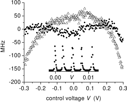
Figure 13: Insert : fraction of recording of the light intensity transmitted by the Fabry Perot interferometer during a temperature controlled laser frequency scan (1 V of control voltage approximately induces changes of 2.5 K in laser temperature and 50 GHz in emitted frequency). Main plot : residues of a linear fit (open triangles) or parabolic fit (solid circles) of all transmitted peak positions.

3.1.2 Zero-field measurements

Results presented in this section have in fact been obtained in the earth field in which Zeeman energy changes are of order 1 MHz or less and thus too small to affect the results given the accuracy of our measurements. A small permanent magnet is placed near the cell to strongly reduce the field homogeneity and thus prevent any nuclear polarisation to build up when the pump beam is absorbed. An example of frequency sweep over the whole ${}^{3}\mathrm{He}$ absorption spectrum is given in figure 14 (${}^{3}\mathrm{He}$ pressure: 0.53 mbar).

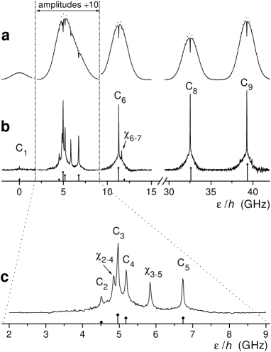
Figure 14: Zero-field saturated absorption spectrum of ${}^{3}\mathrm{He.}$ The upper traces (a) represent the probe absorption signals when the pump beam is applied (solid line) or blocked (dotted line). Traces b and c (an expanded section of trace b) are the difference of probe absorptions with and without the pump beam, with a $\times$4 vertical scale factor. The sections of the spectrum comprising the lines C₂ to C₅ provide a much larger signal and are displayed with a reduced amplitude. Frequency sweep rate is 160 MHz/s, a value ensuring sufficient signal quality and manageable laser frequency drifts. Transition lines are labelled C₁ to C₉, crossover resonances between C_i and C_j are labelled $\chi_{i-j}$. The vertical bars on the axes represent the computed line positions and intensities.

The frequency scale is determined using the accurately known value 3$A_{\mathrm{S}}$/2$=$6.7397 GHz of the C₈-C₉ splitting. The saturated absorption spectrum (solid line in figure 14a) combines the usual broad absorption lines and several narrow dips. The dips reveal a reduced absorption of the probe by atoms interacting with the pump beam. These are atoms with negligible velocity along the beam direction (Doppler-free resonances) or atoms with a velocity such that the Doppler shift is just half of the splitting of two transitions from or to a common level (crossover resonances). An absorption signal recorded without the pump beam (dotted line in figure 14a) only shows the broad features, which can be fit by a Doppler Gaussian profile for isolated lines (e.g. C₈ or C₉). It is used to obtain the narrow resonances in figure 14b by signal substraction. The width $\delta$ of the narrow resonances is 50 MHz FWHM in the conditions of figure 14. It can be attributed to several combined broadening processes, including pump saturation effects and signal acquisition filtering.

Broader line features, the “pedestals” on which narrow resonances stand, result from the combined effects of collisions in the gas. Fully elastic velocity changing collisions tend to impose the same population distribution in all velocity classes, and thus to identically decrease the probe absorption over the whole velocity profile. In contrast, ME collisions involving a ${}^{3}\mathrm{He}$ atom in a gas where the nuclear polarisation is $M$=0 induce a net loss of angular momentum (a uniform population distribution tends to be imposed by the infinite spin temperature, see section 2.2.3). In steady-state, the un-pumped velocity classes will thus acquire only part of the population changes imposed in the pumped velocity class. The relative amplitude of the resulting broad pedestal results from the competition of collisional transfer and collisional loss of orientation. One consequence is that it is almost pressure-independent, as was experimentally checked. Another consequence is that it strongly depends on ${}^{4}\mathrm{He}$ concentration in isotopic mixtures, as illustrated in figure 15.

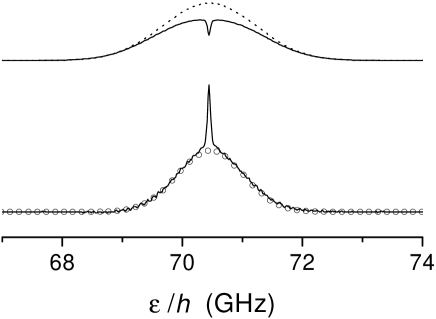
Figure 15: Zero-field saturated absorption spectrum of the D₀ line in a 25% ${}^{3}\mathrm{He}$ - 75% ${}^{4}\mathrm{He}$ mixture (same total pressure, 0.53 mbar, as for figure 14). The lower trace also displays the squared absorption amplitude (open circles), with an arbitrary weight adjusted to fit the saturated absorption pedestal (see text).

The much larger fractional amplitude of the pedestal results from the weaker depolarising effect of the ME collisions: only 25% of the exchange collisions occur in this case with a depolarised ${}^{3}\mathrm{He}$ atom and thus contribute to bleach the pump-induced population changes, while all collisions induce velocity changes. In figure 15 is also displayed the squared absorption profile, which closely matches the shape of the pedestal. This is a general feature also observed in ${}^{3}\mathrm{He}$ spectra, which results from the linear response to the rather low pump power. Assuming that the relative population changes are proportional to the absorbed pump power, frequency detuning reduces by the same Doppler profile factor both these population changes and the probed total population. The resulting squared Doppler profile is still Gaussian, but with reduced width $\Delta/\sqrt{2}.$

From this detailed analysis of the signal shapes we infer two main results. First, very little systematic frequency shift is expected to result from the distortion of the narrow Doppler-free resonances by the broad line pedestals of neighbouring transitions (no shift at all for isolated lines). It can be estimated to be of order $\delta^{2}/\Delta,$ i.e. of order 1 MHz and thus negligible in these experiments. Second, population changes in the whole velocity profile remain limited in pure ${}^{3}\mathrm{He}$ or in ${}^{3}\mathrm{He}$-rich isotopic mixtures. They amount for instance to a 7 % change for the C₉ transition when the pump beam is applied, as illustrated in figure 14 (difference between dotted and solid line). They are significantly larger in a helium mixture, e.g 30 % for the conditions of figure 15. These OP effects on the populations would be reduced for a reduced pump power, and the direct effect of the attenuated ($\div$25) probe itself can be expected to be correspondingly reduced, and hence negligible under similar conditions. However, this would be untrue in pure ${}^{4}\mathrm{He}$ in which strong population relaxation is difficult to impose, and precise absorption or saturated absorption experiments are less conveniently performed. A strong magnetic field would also enhance the perturbing effects of the probe beam, as was discussed in section 2.2.4 and will be demonstrated in section 3.2.4.

A series of identical sweeps including the C₁-C₇ lines, similar to that in figure 14c, was performed to check for reproducibility. The frequency scales were determined using the C₂-C₆ splittings (these transitions connect the two hyperfine levels of the $2^{3}\mathrm{S}$ state to the same excited level, see figure 3, and are thus separated by 6.7397 GHz just as C₈-C₉). To directly probe hyperfine level splittings in the $2^{3}\mathrm{P}$ state we consider the line separations C₂-C₄ and C₃-C${}_{5},$ which directly measure the level energy differences between the lower pairs of $2^{3}\mathrm{P}$ levels (see the zero field level diagram in figure 2). We also consider the separation of the crossover resonances $\chi_{2-4}$-$\chi_{3-5}$, actually computed from differences of the four line positions, which measures an independent energy difference between these levels. Comparison to the values computed using the 3-parameter hyperfine term in the Hamiltonian (section 2.1.3) is shown in figure 16.

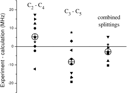
Figure 16: Difference between measured and computed hyperfine splittings in the $2^{3}\mathrm{P}$ state of ${}^{3}\mathrm{He}$ in zero field for selected pairs of individual or combined line splittings (see text). Each closed symbol corresponds to a different experiment. The large open symbols are the statistical averages.

For the two simple splittings, data scatter is $\pm$15 MHz about the average. It is smaller for the third combined splitting, which involves averaging pairs of line position measurements and thus a statistically reduced uncertainty. The three averages have a 6 MHz r.m.s. difference with the computed values, which is consistent with statistical uncertainty. This analysis shows that our unsophisticated spectroscopic measurements are quite accurate and have very little systematic error in the frequency determinations (at most a few MHz over several GHz). It also justifies the use of the correction term beyond the contact interaction term in the hyperfine contribution (equation 6) since our experimental errors are lower than the effect of this correction term (figure 7).

3.1.3 Field effect on line positions

The most obvious effect of an applied magnetic field is to considerably increase the number of observed narrow lines (Doppler-free lines and intercombination lines) in the saturated absorption recordings. For simplicity, we only present in figure 17 selected results for the set of ${}^{3}\mathrm{He}$ lines originating at low field from C₈ and C${}_{9}.$ These are the most efficient optical transitions for OP of ${}^{3}\mathrm{He}$, and thus are of special interest. Furthermore, the analyses of transition intensity measurements described in sections 3.2.2 and 3.3 request an accurate knowledge of all line positions for these transitions.

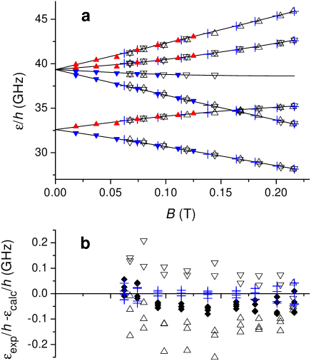
Figure 17: a : Plot of frequency shifts on the ${}^{3}\mathrm{He}$ $\mathrm{C}_{8}$ and $\mathrm{C}_{9}$ lines in an applied magnetic field measured by a saturated absorption technique. Solid lines : computed Zeeman shifts (same as in figure 6). Up and down triangles : data for $\sigma_{+}$ and $\sigma_{-}$ polarisations of light beams. Solid and open symbols : measurement using the air-core and iron yoke magnets respectively. Crosses : result of corrections applied the open symbol data set (see text). b : Differences between experimental and computed values for the measurements in the iron yoke magnet are plotted as a function of $B.$ Open symbols : raw data (no correction) ; filled symbols : data with field corrections only ; crosses : data with field and frequency corrections (see text).

To reduce the number of observed lines and thus facilitate data processing, the same circular polarisation ($\sigma_{+}$ or $\sigma_{-}$) was used for the pump and the probe beam, and two measurements were thus performed for each field value. For the higher field data (iron yoke magnet, open symbols in figure 17a) the use of an imperfect circular polarisation made it possible to usually observe all intense lines in each measurement. Zero field scans were performed between measurements to evaluate the slow drift of the laser frequency and provide reference measurements for the Zeeman shifts.

For the measurements in the air-core magnet (up to 0.125 T), the agreement between computed and measured line positions $\epsilon/h$ is fair, but affected by fluctuating frequency offsets. The r.m.s. differences are quite large (50 MHz and 110 MHz for $\sigma_{+}$ and $\sigma_{-}$ probes respectively), but the largest contribution to these differences can be attributed to a global frequency offset from scan to scan. Estimating the offset of each scan from the average of the 3 recorded line positions, the remaining differences are significantly reduced (9 MHz r.m.s. for $\sigma_{+}$ and $\sigma_{-}$). The accuracy of these line position measurements is thus comparable to that of the zero-field measurements (figure 16).

For the measurements in the iron yoke electromagnet (up to 0.25 T), a similar frequency offset adjustment is not sufficient to significantly reduce the differences between measured and computed line positions (figure 17b). For instance, they amount to 130 MHz r.m.s. for the $\sigma_{+}$ measurements (open up triangles). Moreover, splittings within a given scan consistently differ from the computed ones. Assuming that the magnetic field is not exactly proportional to the applied current due to the presence of a soft iron yoke in the magnet, we use the largest measured splitting on the C₉ line (the transitions originating from the sublevels $m_{F}$=$\pm$3/2) to determine the actual value of the magnetic field during each scan. Solid symbols in figure 17b are computed differences for these actual values of the magnetic field. Crosses (figures 17a and 17b) correspond to fully corrected data, allowing also for frequency offset adjusments. The final remaining differences (22 MHz r.m.s.) are still larger than in the air-core magnet, yet this agreement is sufficient to support our field correction and offset adjustment procedures in view of the line intensity measurements described in the following section.

3.2 Line intensities

3.2.1 Experimental setup

The experimental arrangement is either the one sketched in figure 12, in which the pump beam is blocked and only a weak probe beam (usually 0.1-1 mW/cm²) is transmitted through the cell, or a simplified version of the setup when no saturated absorption measurement is performed.

The magnetic field is obtained by different means depending on its intensity. Data at moderate field (up to 0.22 T) data have been acquired using the resistive magnets described in section 3.1.1. Higher field measurements have been performed in the bore and fringe field of a 1.5 T MRI superconducting magnet CIERM . With the laser source and all the electronics remaining in a low-field region several meters away from the magnet bore, cells were successively placed at five locations on the magnet axis with field values ranging from $B$=6 mT to 1.5 T. The 1.5 T value (in the bore) is accurately known from the routinely measured ${}^{1}\mathrm{H}$ NMR frequency (63.830 MHz, hence 1.4992 T). The lower field intensities, 6 mT and 0.4 T, have been measured using a Hall probe with a nominal accuracy of 1%. The intermediate values, 0.95 T and 1.33 T, are deduced from the measured Zeeman splittings with a similar accuracy of 1%. Due to the steep magnetic field decrease near the edge of the magnet bore, large gradients cause a significant inhomogeneous broadening of the absorption lines in some situations discussed in section 3.2.3. For these high field measurements, the Fabry Perot interferometer was not implemented and no accurate on-site check of the laser frequency scale was performed. Instead, the usual corrections determined during the saturated absorption measurements (see section 3.1.1 and figure 13) are used for the analysis of the recorded absorption spectra.

A systematic study of the effect of experimental conditions such as gas pressure, RF discharge intensity, and probe beam power and intensity, has been performed both in low field (the earth field) and at 0.08 T. The main characteristic features of the recorded spectra have been found to be quite insensitive to these parameters. Absorption spectra have been analysed in detail to accurately deduce the relative populations of different sublevels (from the ratios of line intensities) and the average atomic density of atoms in the $2^{3}\mathrm{S}$ state in the probe beam (from its absorption). A careful analysis of lineshapes and linewidths reveals three different systematic effects which are discussed in the next three sections.

3.2.2 Effect of imperfect ${}^{3}\mathrm{He}$ isotopic purity

Evidence of a systematic effect on absorption profiles was observed in experiments with nominally pure ${}^{3}\mathrm{He}$ gas. A typical recording of the C₈ and C₉ absorption lines for $B$=0 and residuals to different Gaussian fits are shown in figure 18.

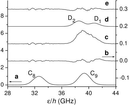
Figure 18: Zero-field absorption measurement on the C₈ and C₉ lines in nominally pure ${}^{3}\mathrm{He}$ at 0.53 mbar. a : absorption signal (the vertical scale is 20 times less sensitive than for the other traces). b : residue plot of independent Gaussian fits to the two lines. c : residue plot of the same fit as in plot b for C₈ and the corresponding computed C₉ profile. d : computed D₂-D₁ profile with a $\div$200 amplitude scaling corresponding to the measured traces of ${}^{4}\mathrm{He}$ (see text). e : residue plot of independent Gaussian fits to the two lines after correction for the ${}^{4}\mathrm{He}$ contribution.

A straightforward fit by two independent Gaussian profiles to the recorded lines (trace a) systematically provides a 1.5-2 % larger width and an unsatisfactory fit for the C₉ transition (trace b, residue plot). Moreover, the ratio of fitted line strengths (areas) is 7.8% larger than the value computed using table 9 in the Appendix (1.374 instead of 1.274). Conversely, fitting on the C₈ component and assigning the expected linewidth, amplitude and frequency shift to the C₉ component provides the residue plot of trace c, which suggests the existence of an additional contribution to absorption. All this is explained by the presence of traces of ${}^{4}\mathrm{He}$, which are independently observed by absorption measurements on the isolated D₀ line. Indeed this small amount of ${}^{4}\mathrm{He}$ (isotopic ratio $R$=0.2 to 0.5 %) affects the absorption measurement performed on ${}^{3}\mathrm{He}$ due to the intense lines which lie within one Doppler width of the C₉ line (trace d: computed absorption lines of  ${}^{4}\mathrm{He}$ for $R$=0.2 %). The reduction of the ${}^{3}\mathrm{He}$ gas purity is attributed to the cell cleaning process, which involves several strong discharges performed in ${}^{4}\mathrm{He}$ prior to final filling with pure ${}^{3}\mathrm{He}$. Reversible penetration of helium into the glass walls is believed to be responsible for the subsequent presence of a small (and surprisingly unsteady) proportion of ${}^{4}\mathrm{He}$ in the gas. When the appropriate correction is introduced to substract the contribution of ${}^{4}\mathrm{He}$ lines from the absorption spectra, the fit by two independent Gaussian profiles is significantly improved (trace e) and the linewidths are found to be equal within $\pm$0.2 %. For the recording of figure 18a one obtains a Doppler width $\Delta$=1.198 GHz, corresponding to a temperature of 304 K in the gas (consistent with the ambient temperature and the power deposition of the RF discharge in the plasma).

The ratio of the line amplitudes after this correction is closer to the ratio of computed transition intensities, still 3.5$\pm$0.2% larger in this example. A series of measurements performed in a row provides very close results, with a scatter consistent with the quoted statistical uncertainty of each analysis. In contrast, a measurement performed in the same cell after several days may lead to a different proportion of ${}^{4}\mathrm{He}$ and a different ratio of transitions intensities (for instance $R$=0.35% and a ratio of intensities 2.9$\pm$0.1% smaller than the computed one).

Consequences of the presence of a small proportion of ${}^{4}\mathrm{He}$ on the lineshapes and intensities of recorded spectra are indeed also observed in an applied magnetic field, as shown in figure 19 for $B$=0.111 T.

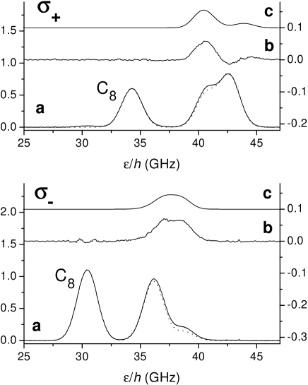
Figure 19: Absorption measurements on the C₈ and C₉ lines performed in a field $B$=0.111 T in nominally pure ${}^{3}\mathrm{He}$ at 0.53 mbar for circular polarisations (upper graph : $\sigma_{+}$, lower graph : $\sigma_{-}$). Traces a correspond to the raw absorption signals (solid lines) and computed profiles (dotted lines, see text). Traces b are differences (residue plots) between absorption signals, corrected for light polarisation defects, and computed profiles. Traces c are the computed profiles for pure ${}^{4}\mathrm{He}$, scaled down in order to correspond to an isotopic ratio $R$=0.4%. Expanded vertical scales ($\times$5, right hand side axes) are used for traces b and c.

The recorded absorption signals are similar to the computed ones (dotted lines), but two significant differences appear. First, a small line is visible for instance in the upper graph around $\varepsilon/h$=30 GHz, where no $\sigma_{+}$ transition should be observed. This is due to an imperfect circular polarisation of the probe beam in the cell, resulting in part from stress-induced circular dichroism in the cell windows (measured to be of order 0.2%). The amount of light with the wrong polarisation is determined for each recording, and each signal is corrected by substracting the appropriate fraction of the signal with the other circular polarisation (0.79% and 0.18% corrections for $\sigma_{+}$ and $\sigma_{-}$ recordings in figure 19). Second, the corrected signals may then tentatively be fit by the sum of three Gaussian profiles centred on the frequencies independently determined in a saturated absorption experiment (see figure 17). But, as is the case in zero field, this procedure does not provide satisfactory results for the amplitudes and linewidths of the split C₉ lines (corresponding to the transitions originating from any of the lowest levels of the $2^{3}\mathrm{S}$ state, A₁ to A₄, to the highest levels of the $2^{3}\mathrm{P}$ state, B₁₇ and B₁₈). In figure 19, traces b display the differences between the corrected signals and the computed sums of three Gaussian profiles with a common linewidth and with amplitudes proportional to the nominal transition probabilities in this field. Two global amplitudes and the linewidth ($\Delta$=1.221 GHz) are adjusted to fit the two C₈ transitions, and the resulting differences are best accounted for assuming a proportion $R$=0.4% of ${}^{4}\mathrm{He}$ in the gas (traces c in figure 19). In order to better reproduce the experimental recordings, the amplitudes of the split C₉ lines are finally allowed to vary. Fits with excellent reduced $\chi^{2}$ and no visible feature in the residues are obtained and the obtained ratios of intensities are given in table 1 for this typical recording .

polarisation $\sigma_{-}$ $\sigma_{+}$ computed $T_{6,18}$ $T_{5,17}$ C₈ intensity 0.3757 0.18803 computed $T_{4,17}$ $T_{3,18}$ $T_{2,17}$ $T_{1,18}$ C₉ intensity 0.31311 0.04731 0.16111 0.25107 C₈/C₉ comp. 0.83340 0.12592 0.85683 1.33527 ratio meas. 0.85198 0.15275 0.86360 1.30055 deviation +2.2 % +21 % +0.8 % $-$3.6 %

Table 1: Computed line intensities $T_{ij}$ for $B$=0.1111 T and their ratios are compared to the experimental line amplitude ratios of figure 19.

The same kind of discrepancy as in zero field is obtained for the strong components of the transitions; it happens to be much worse for the weakest line in some recordings, including that of figure 19, for reasons which are not understood.

In an attempt to test whether the remaining line intensity disagreements with the computed values may result from imperfect corrections for the presence of ${}^{4}\mathrm{He}$, or from difficulties due to fitting several overlapping lines, we have also probed the well resolved $\mathrm{D}_{0}$ line of ${}^{4}\mathrm{He}$ in a gas mixture in the 0-0.12 T field range. Using a circularly polarised probe beam, the two transitions connecting levels Y₁ and Y₃ to Z₉ ($\sigma_{+}$ and $\sigma_{-}$ polarisations respectively) are split in frequency by 56 GHz/T (see section 2.1.2). The ratio of the corresponding line intensities is computed to be approximately given in this field range by:

$$T_{3,9}^{(4)}/T_{1,9}^{(4)}\approx 1+1.88B+2.02B^{2},$$ (45)

where $B$ is the field intensity in Tesla. The results of a series of absorption measurements for a transverse probe beam (with linear perpendicular polarisation) are displayed in figure 20.

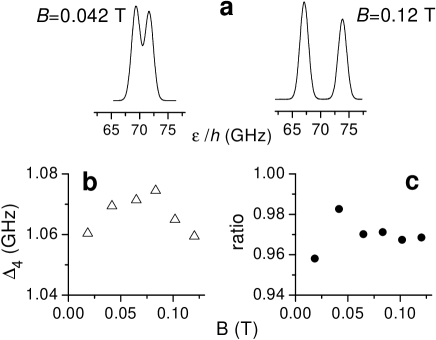
Figure 20: Absorption measurements on the D₀ line of ${}^{4}\mathrm{He}$ performed in fields up to $B$=0.12 T with a lin$\bot$ polarised probe beam in a ${}^{3}\mathrm{He}$-${}^{4}\mathrm{He}$ mixture at 0.53 mbar (isotopic ratio $R$=3). a : Recordings of absorption signals are given for two values of the field. The lower plots display the results of Gaussian fits to the signals. b : Doppler width $\Delta_{4}$, c : ratios of measured to computed relative line amplitudes $\left(A_{\sigma+}/A_{\sigma-}\right)/\left(T_{3,9}^{(4)}/T_{1,9}^{(4)}\right).$

The absorption signals are fit by the sum of three Gaussian profiles centred on the transition frequencies (measured in a saturated absorption experiment). This allows for a small amount of $\pi$ polarisation in the probe beam, which experimentally arises from imperfect alignment of the direction of the polarisation with respect to $B.$ In spite of this drawback, the transverse probe beam configuration is preferred to a longitudinal one, for which polarisation defects may directly affect the ratio of line amplitudes.

The common linewidth $\Delta_{4}$=1.067 $\pm$0.006 GHz (figure 20b, corresponding to a temperature of 321 K) is found to be independent of the field. The ratio $A_{\sigma+}/A_{\sigma-}$ of the measured line amplitudes for the $\sigma_{+}$ and $\sigma_{-}$ polarisation components is found to increase with $B$ as expected from equation 45, with however a slightly lower value ($\sim$3%, figure 20c).

To summarise the results of this section, the difference of measured line intensities in our experiments with respect to the computed ones is usually small (of order $\pm$3%) after correcting for the presence of some ${}^{4}\mathrm{He}$ in our ${}^{3}\mathrm{He}$ cells and for the observed light polarisation imperfections. This difference does not arise from signal-to-noise limitations and its origin is not known. This may set a practical limit to the accuracy with which an absolute measurement of population ratios can be made using this experimental technique. Similar discrepancies are also observed at higher fields, situations for which the additional systematic effects described in the following sections must first be discussed.

3.2.3 Effects of magnetic field gradients

As previously mentioned (section 3.2.1), absorption experiments above 0.25 T have been performed in the fringe field of a 1.5 T magnet. The exact field map of this magnet was not measured, but the field decreases from 1.33 T to 0.95 T in only 25 cm, so that field gradients along the axis may exceed 15 mT/cm at some locations. In contrast, field variations in transverse planes are much smaller in the vicinity of the field axis. As a result, a negligible broadening of absorption lines is induced by the field gradient for perpendicular probe beams ($\sigma$ or $\pi$ polarisation for a linear polarisation perpendicular or parallel to $B$). For probe beams propagating along the field axis ($\sigma$ polarisation for a linear polarisation, $\sigma_{+}$ or $\sigma_{-}$ polarisation for a circular polarisation), the range of fields $\delta B$ applied to the probed atoms is the product of the field gradient by the cell length. This field spread $\delta B$ induces spreads $\delta\epsilon_{ij}/h$ of optical transition frequencies which are proportional to $\delta B$ and to the derivatives $d\epsilon_{ij}/dB.$ Each spread $\delta\epsilon_{ij}/h$ thus depends on the probed transition as illustrated in figure 21 for $B$=0.95 T.

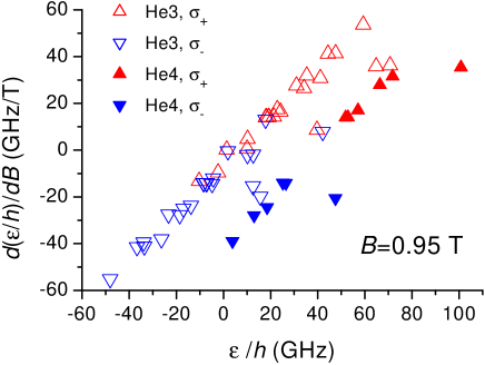
Figure 21: Computed field-derivatives of the transitions energies $\epsilon_{ij}/h$ are plotted for all ${}^{3}\mathrm{He}$ and ${}^{4}\mathrm{He}$ circular polarisation transitions as a function of $\epsilon_{ij}/h$ for $B$=0.95 T. Inhomogeneous line broadenings proportional to these values are induced by a field gradient.

The resulting absorption profiles are given by the convolution of the Doppler velocity distribution and of the frequency spread functions, computed from the density distribution of metastable atoms, the field gradient at the cell location and the derivatives $d\epsilon_{ij}/dB.$ Assuming for simplicity a uniform density of atoms in the $2^{3}\mathrm{S}$ state, computed broadened absorption profiles only depend on the dimensionless ratio $\delta\epsilon_{ij}/h\Delta$ of the transition frequency spread to the Doppler width. Figures 22a and 22b display examples of computed profiles (absorption as a function of this reduced detuning).

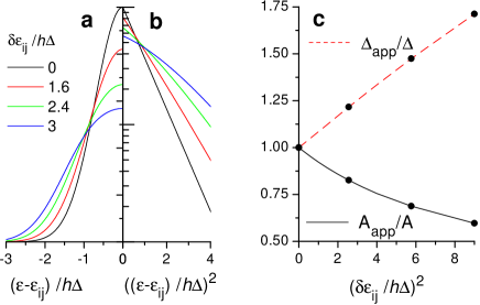
Figure 22: a : Computed absorption (half-)profiles in a magnetic field gradient resulting from the convolution of a Gaussian Doppler profile (width $\Delta$) and of a uniform spread of the resonance frequency (over a width $\delta\epsilon_{ij}/h$). b : The same profiles are plotted in semi-logarithmic scale as a function of the square of the detuning. A Gaussian profile appears as a straight line. c : Apparent linewidths $\Delta_{app}$ and amplitudes $A_{app}$ of these computed profiles are plotted as a function of the square of the reduced resonance frequency spreads. The solid symbols correspond to the profiles displayed in a and b.

For increasing frequency spreads, profiles become broader and their maximum amplitude decreases (the area is strictly independent of $\delta\epsilon_{ij}/h\Delta$). Deviation from a true Gaussian profile is more clearly seen in figure 22b as a deviation from a straight line. To test the procedure used in the analysis of experimental data, one may fit a Gaussian function to these computed profiles. The apparent linewidths and amplitudes thus obtained, $\Delta_{app}$ and $A_{app},$ are plotted in figure 22c. For small frequency spreads, $\Delta_{app}$ and $1/A_{app}$ are almost proportional to $\delta\epsilon_{ij}^{2}.$ However, significant deviations appear at large $\delta\epsilon_{ij}$, and the product $\Delta_{app}A_{app}$ is not strictly constant (it increases by 2 % for $\delta\epsilon_{ij}/h\Delta\sim$3). This means that whenever frequency spreads cannot be avoided (e.g. using a transverse probe beam), fitting procedures to Gaussian profiles introduce systematic errors. Computation of line areas would provide the true line intensities, but this procedure cannot be used to separately obtain the intensities of ill-resolved transitions.

Figure 23 displays part of an absorption measurement performed at $B$=0.95 T with a longitudinal $\sigma$-polarised probe beam.

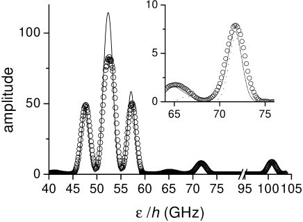
Figure 23: Part of an absorption spectrum recorded at $B$=0.95 T in a ${}^{3}\mathrm{He}$-${}^{4}\mathrm{He}$ mixture at 2.13 mbar (isotopic ratio $R$=3) using a longitudinal probe beam (open symbols). The solid curve is the spectrum computed for this $R,$ assuming thermal Doppler widths for the different lines. Its amplitude is scaled to reproduce that of the 47 GHz line. Experimental broadening of the absorption lines is directly found on the 101 GHz line, and suggested by the residual absorption between the main lines (non-zero signal at 50 and 55 GHz), which is 2-3 times larger than computed. The insert is an expanded portion of the spectrum, in which several ${}^{3}\mathrm{He}$ and ${}^{4}\mathrm{He}$ lines overlap (the computed absorption of pure ${}^{4}\mathrm{He}$ is displayed as a dotted line). Experimental broadening of the absorption lines also clearly appears for this part of the spectrum.

It includes the two split D₀ transitions connecting levels Y₁ and Y₃ to Z₉ : the $\sigma_{+}$ ${}^{4}\mathrm{He}$ line with highest $\epsilon/h$ (101 GHz), and $\sigma_{-}$ ${}^{4}\mathrm{He}$ line with highest $\epsilon/h$ (47 GHz), respectively. The recorded absorption signal (symbols) roughly correspond to the profile computed assuming the nominal Doppler widths $\Delta$ and neglecting frequency spreads (solid line). Clear amplitude differences are however observed, in particular for the most intense line. They can be attributed to OP effects, and will be discussed in detail in the next section (3.2.4). Moreover, significant linewidth differences appear, for instance on the isolated most shifted ${}^{4}\mathrm{He}$ line (fitted apparent linewidth $\Delta_{app}$=1.42 GHz, 30% larger than $\Delta_{4}$). Most of the other lines actually result from the overlap of several atomic transitions, and a straightforward Gaussian fit is not relevant. For example, the computed total absorption around $\epsilon/h$=72 GHz (insert in figure 23, solid line) results from the two ${}^{4}\mathrm{He}$ transitions at 66.7 and 72.1 GHz (dotted line) and the two ${}^{3}\mathrm{He}$ transitions  at 65.2 and 71.1 GHz.

To better analyse the effect of the probe beam direction on the shape and widths of different lines, we plot in figure 24 the absorption data using the same method as in figure 22b.

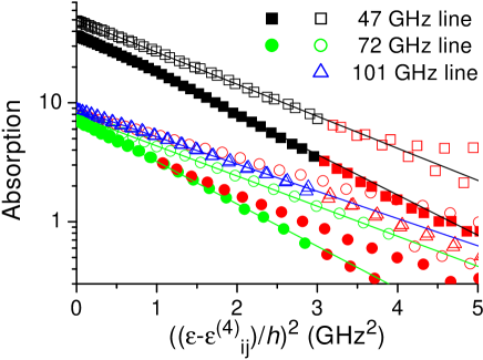
Figure 24: Semi-logarithmic plot of absorption data recorded at $B$=0.95 T in a ${}^{3}\mathrm{He}$-${}^{4}\mathrm{He}$ mixture at 2.13 mbar (isotopic ratio $R$=3). They are presented for 3 different ${}^{4}\mathrm{He}$ lines as a function of the square of the frequency mistuning $\left(\epsilon-\epsilon_{ij}^{(4)}\right)/h.$ Open symbols : data of figure 23, longitudinal probe beam. Solid symbols : data for a transverse probe beam. The straight lines represent Gaussian absorption profiles, and the values of their slopes are used to extract the apparent linewidths $\Delta_{app}.$ The smallest linewidths, consistent with the ${}^{4}\mathrm{He}$ Doppler width, are obtained for a transverse probe ($\Delta_{4}$=1.13 and 1.105 GHz for the 47 and 72 GHz lines). Larger apparent linewidths are obtained for a longitudinal probe ($\Delta_{app}$=1.27, 1.31 and 1.42 GHz for the 47, 72 and 101 GHz lines).

The open symbols correspond to three of the lines in figure 23, with a probe beam along the direction field, and the solid symbols to lines from a similar recording with a perpendicular probe beam. Apart from the asymmetries on the 71 GHz lines which result from the additional ${}^{3}\mathrm{He}$ line on the low-frequency side of the absorption profile (which is thus not retained in the analysis), satisfactory linear fits reveal Gaussian-like profiles and provide the values of the corresponding linewidths. The experiments performed with a transverse probe provide data with the steepest slopes and hence the smallest linewidths, while those using a longitudinal probe lead to larger apparent linewidths as expected . Using the convolution results of figure 22c, the frequency spreads $\delta\epsilon_{ij}/h$ for these lines are computed to be 1.4, 1.65 and 1.85 GHz respectively. From the derivatives $d\epsilon_{ij}/dB$ for these transitions (figure 21), one computes that a field spread $\delta B$=52 mT would produce frequency spreads of 1.08, 1.65 and 1.85 GHz, corresponding to the observed broadenings for the 72 and 101 GHz lines. The additional apparent broadening for the 47 GHz experimental line may be attributed to OP effects for this rather intense line (see the next section 3.2.4). For the estimated value of the field gradient (15 mT/cm), this 52 mT field spread would be obtained for an effective cell length of 3.5 cm. This is quite satisfactory since the density of atoms in the metastable $2^{3}\mathrm{S}$ state vanishes at the cell walls, so that most of the probed atoms lie within a distance shorter than the actual gap between the end windows of our 5 cm-long cells (external length).

To summarise the results obtained in this section, the expected effects of strong field gradients on absorption lines have indeed been observed. They introduce a systematic broadening and amplitude decrease of absorption signals which can be significant (up to 30 % changes in our experiments), and must be considered in quantitative analyses. For isolated lines, area measurements are not affected by the transition frequency spreads. However, most lines usually overlap in a recorded absorption spectrum (especially in an isotopic mixture), and the quantitative analysis of such spectra is in practice too inaccurate if the different linewidths are not known. It is thus important to only use a transverse probe beam configuration whenever accurate absorption measurements are needed and a field gradient is present. The same argument would also apply to saturated absorption measurements, for which even limited frequency spreads (e.g. of order 100 MHz) would strongly decrease the signal amplitudes.

3.2.4 Effects of optical pumping

A comparison of absorption recordings at $B$=0 and 1.5 T is presented in figure 25.

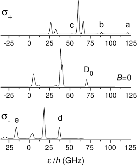
Figure 25: Recordings of complete absorption spectra at $B$=0 and 1.5 T for circular polarisations in a ${}^{3}\mathrm{He}$-${}^{4}\mathrm{He}$ mixture at 2.13 mbar (isotopic ratio $R$=3). The lines labelled a to e are especially considered in the analysis of OP effects. The ${}^{4}\mathrm{He}$ transitions with the highest energy (involving the Z₉ level) considered in figure 20 for moderate fields are labelled a and d at 1.5 T, and correspond to the D₀ line at zero field. The assignment of the lines at zero field can be made using figure 3.

As expected in such a high magnetic field, the absorption spectra are deeply modified and strongly depend on the probe light polarisation. Line shifts of order of the fine structure splittings, and large changes in the intensities of the absorption lines are observed, for instance on the well-resolved transitions to the excited Z₉ level (labelled a, D₀ and d in figure 25, which we shall generically call D₀ transitions). For these lines, the computed transition intensities and the corresponding weights in the total spectra are given in table 2.

line d  (D₀, $\sigma_{-}$) D₀ ($B$=0) a  (D₀, $\sigma_{+}$) $T_{i9}$ 0.7722 0.3333 0.06459 weight (calc.) 19.31 % 8.333 % 1.615 % weight (exp.) 16.6 % 7.9 % 1.8 %

Table 2: Computed line intensities $T_{i9}$ of the D₀ line for $B$=0 and 1.5 T. The weights in the spectra (fraction of the line area over the total area) are computed for an isotopic ratio $R$=3 corresponding to the experimental conditions. The last line displays the experimental weights for the measurements shown in figure 25.

It is not possible to directly compare absorption signals at $B$=0 and 1.5 T because the plasma intensity and distribution in the cell are strongly modified in high field. However, according to the sum rules of equation 10, the average density of atoms in the $2^{3}\mathrm{S}$ state along the probe beam is deduced by integrating the absorption signal over the whole spectrum. This is used to scale the absorption amplitudes in figure 25 and have a meaningful comparison of line weights in table 2. While there is a satisfactory agreement with expectations for all line weights at $B$=0, the ratio of the weight of the strong (D${}_{0},$ $\sigma_{-}$) absorption line d to that of the weak (D${}_{0},$ $\sigma_{+}$) line a is substantially smaller than computed.

The measurements displayed in figure 25 have been performed with a rather intense probe beam, so that OP effects may play a significant role. As for all experiments performed in low field, we can assume that OP creates no nuclear polarisation $M$ for the ground state ${}^{3}\mathrm{He}$ atoms. It is not possible to enforce rapid nuclear relaxation as is done in low field (section 3.1.2) by imposing a strong relative field inhomogeneity at 1.5 T. However the angular momentum deposited in the cell by the absorption of a fraction of the probe beam could only lead to a very slow growth rate of $M$ for our experimental conditions. As a result, only a very small nuclear polarisation $M$ can be reached in a frequency sweep during the time spent on an absorption line ($\sim$5 s). Negligible changes of the Zeeman populations and hence of absorption signal intensities are induced by this process. In contrast, the OP effects in the $2^{3}\mathrm{S}$ metastable state described in section 2.2.4 may have a strong influence on the distribution of the Zeeman populations, and thus significantly decrease the absorption (see figure 10).

To discuss and analyse in detail these OP effects at 1.5 T, we show in figure 26 (symbols) parts of the experimental spectra extracted from figure 25, together with different computed profiles which are discussed below.

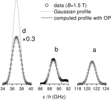
Figure 26: Expanded plot of selected absorption profiles from experimental recordings at 1.5 T (open symbols). The labelling of the lines is that of figure 25. The vertical scale has been reduced ($\times$0.3) for the strongest line d (the actual ratio of the maximum absorptions of lines d and a is 7.0). Dotted lines : computed Gaussian profiles for these transitions. Solid lines : computed profiles taking into account OP effects with the parameters given in the text (hardly distinguishable from the dotted Gaussian profiles for lines a and b).

It is important to note that in spite of the double-pass configuration in the cell used to enhance absorption signals, no narrow saturated absorption dips appear in the data. This is different from what is observed at low field when a counterpropagating pump beam induces population changes in a given velocity class, and when velocity changing collisions only partly redistribute these changes over the whole Doppler profile (see section 3.1.2 and figures 14 - 15). We shall thus assume that in the conditions of figure 25 no correlation is introduced by the probe beam between atomic velocity and Zeeman population changes, i.e. that any out-of-equilibrium orientation produced by OP due to the probe is uniformly redistributed among all atoms in the Doppler profile. The pumping time $\tau_{p}$ introduced in equations 42 and 43 can thus be computed from the photon absorption rates defined in equations 2 and 9 using an averaging procedure similar to that of Nacher85 . The averaging is performed over the atomic velocity projection $v$ along the probe beam, which introduces the Doppler shift $\omega v/c$ for the atomic transition angular frequencies $\omega$=$\omega_{ij}^{(4)}$ and $\omega_{ij}$ in equations 2 and 9. For ${}^{3}\mathrm{He}$ transitions, one obtains:

$$\frac{1}{\tau_{p}}=\frac{4\pi\alpha f}{m_{e}\omega\Gamma^{\prime}}~{}~{}\frac{T_{ij}I_{las}}{\bar{v}\sqrt{\pi}}\int_{-\infty}^{\infty}\frac{\left(\Gamma^{\prime}/2\right)^{2}e^{-(v/\bar{v})^{2}}dv~{}}{\left(\Gamma^{\prime}/2\right)^{2}+\left(\omega-\omega_{ij}-\omega_{ij}v/c\right)^{2}}$$ (46)

where the mean velocity $\bar{v}=2\pi c\Delta_{3}/\omega_{ij}$ is related to the Doppler width defined in equation 44. For a single-frequency laser and a small enough damping rate of the optical transition coherence ($\Gamma^{\prime}/2\ll 2\pi\Delta_{3}$), the integral is easily computed:

$$\frac{1}{\tau_{p}}\simeq\frac{\sqrt{\pi}\alpha f}{m_{e}\omega\Delta_{3}}~{}T_{ij}I_{las}~{}e^{-(\left(\omega-\omega_{ij}\right)/2\pi\Delta_{3})^{2}}.$$ (47)

A similar result is obtained for ${}^{4}\mathrm{He}$ transitions by substitution of $\Delta_{4},$ $T_{ij}^{(4)}$ and $\omega_{ij}^{(4)}$ in equation 47. The numerical value of the first factor appearing in the pumping rate expression is for ${}^{4}\mathrm{He}$:

$$\frac{\sqrt{\pi}\alpha f}{m_{e}\omega\Delta_{4}}~{}=4.269\times 10^{3}~{}\mathrm{s}^{-1}/(\mathrm{W/m}^{2}),$$ (48)

and it is 15 % smaller for ${}^{3}\mathrm{He}$ due to the larger value of the Doppler width.

For a given laser intensity, the pumping rate is thus expected to be proportional to the transition intensity $T_{ij}$ and, for each absorption line, to decrease with increasing detuning from transition frequencies of atoms at rest. Relying on the OP model of section 2.2.4, Zeeman populations can be numerically computed as a function of the pumping rate. The absorption signals, which are proportional to the probed populations, to $T_{ij}$ and to the Gaussian factor in equation 47, can then in principle be computed using a single global scaling parameter (the number density of atoms in the $2^{3}\mathrm{S}$ state).

In our experiments, the laser intensity $I_{las}$ of the probe beam at the cell location could not be precisely measured, and instead was deduced from the comparison of the measured ratio of the maximum absorptions of the $\sigma_{-}$ and $\sigma_{+}$ D₀ lines, labelled d and a in figures 25 and 26, to the computed ratio which would be obtained in the absence of OP effects, i.e. for $y_{1}$=$y_{3}$=1/3 ($y_{3}T_{3,9}/y_{1}T_{1,9}$=7.0 instead of $T_{3,9}/T_{1,9}$=11.96). The value $\left(\tau_{e}/\tau_{p}\right)/T_{ij}$=3.28$\times$10^-3 is numerically obtained from this comparison of OP effects on these lines at resonance (the two values for $T_{ij}$ are given in table 2). The exchange rate $1/\tau_{e}$ is computed using equation 27 and the value of the exchange rate $1/\tau_{e}^{0}$ in a pure ${}^{3}\mathrm{He}$ gas at the operating pressure(3.75$\times$10⁶ s^-1/mbar JDR71 ):

$$1/\tau_{e}=1/\tau_{e}^{0}\left(1+R\left(\mu-1\right)\right).$$ (49)

For the conditions of the experiment (isotopic ratio $R$=3, total pressure 2.13 mbar) $\tau_{e}$=1.04$\times$10^-7 s, hence $1/(\tau_{p}T_{ij})$ =3.15$\times$10⁴ s and $I_{las}$=7.4 W/m² or 0.74 mW/cm², which is quite consistent with its independently estimated value. For this value of $I_{las},$ OP effects are computed for all lines as a function of the detuning from resonance, and the resulting absorption profiles precisely agree with the experimental data (figure 26, solid lines, compared to the Doppler profiles, dotted lines). This agreement over the whole profiles is better seen in figure 27.

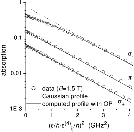
Figure 27: Semi-logarithmic plot of absorption data (open symbols) recorded at $B$=1.5 T in a ${}^{3}\mathrm{He}$-${}^{4}\mathrm{He}$ mixture at 2.13 mbar (isotopic ratio $R$=3). They are presented for 3 different ${}^{4}\mathrm{He}$ lines (D₀, 3 light polarisations) as a function of the square of the frequency detuning $\epsilon/h-\epsilon_{ij}^{(4)}/h.$ The dotted straight lines represent gaussian absorption profiles, the solid lines are the computed profiles with OP effects (see text).

There is a slight systematic deviation for all lines at large detuning, where absorption is larger than computed. This may be due to a temperature slightly above room temperature (as is systematically observed in other experiments), and to the difference between the true atomic (Voigt) profile and a Gaussian one. The agreement is otherwise very good and fully supports the collisional redistribution assumption used to derive equation 47. These measurements can also be viewed as indirect checks of the variation of the population of the pumped sublevel with the pumping rate, such as plotted in figures 10 and 11, up to a 45 % population reduction for $y_{3}$. The influence of $I_{las}$ was indeed also directly measured by using a linear $\sigma$ polarisation instead of a circular one, thus reducing the effective pump power by a factor 2 on isolated lines. All measured OP effects are reduced according to calculations, with for instance a 29 % maximum population reduction for $y_{3}$ on the $\sigma_{-}$ D₀ line.

OP effects for other transitions also agree with expectations. For instance, probing the population $y_{2}$ with a $\pi$ polarisation (figure 27) induces relatively small OP effects in spite of a significant transition intensity. This is consistent with the reduced sensitivity of the Y₂ state to OP which was noticed in section 2.2.4 (figure 11). Most ${}^{3}\mathrm{He}$ transitions are difficult to analyse due to the proximity of several overlapping lines, but the lines c and e in figure 25 can be considered to evaluate OP effects. Line c is an isolated line probing the A₅ state, so weak that no significant OP effect is expected (a 0.2 % maximum population reduction for $a_{5}$), and observed. In contrast, line e consists of 4 lines (two with $\epsilon/h\sim$-16.1 GHz, two with $\epsilon/h\sim$-14.9 GHz), each with a transition intensity $\sim$1. Experimentally, the ratio of the maximum absorptions of lines e and c is 40.2, 4 % lower than expected from transition intensities, thus suggesting a 4 % relative decrease of the probed populations. However these transitions concern 4 different sublevels in the $2^{3}\mathrm{S}$ state, this is an average decrease for the populations in these sublevels. Furthermore, the simple OP model of section 2.2.4 cannot be directly applied since it assumes that a single level is pumped. Still, if the A₅ state alone was pumped with the probe intensity used in the experiment, a computed 3.2 % maximum population reduction would be obtained for $a_{5}$, in reasonable agreement with the small observed OP effects.

Let us finally mention that OP effects have been observed to have all the expected features at lower magnetic field. For instance, for the same laser intensity $I_{las}$ as at 1.5 T, the maximum population reduction for $y_{3}$ on the (D₀, $\sigma_{-}$) line is 38 % at 1.3 T, 26 % at 0.95 T and 8 % at 0.4 T. The much weaker effects expected for other transitions could not clearly be observed, especially in the presence of strong field gradients which also affect the apparent line intensities and shapes as discussed in the previous section.

To summarise the results of this section, the computed effects of optical pumping in the $2^{3}\mathrm{S}$ state have been observed and quantitatively verified in some detail. This supports the validity of the assumptions made on the effect of metastability exchange collisions on the Zeeman populations and of the simple OP model considered in section 2.2. It also confirms that orientation is fully redistributed by collisions over the whole velocity profile in high field. This can be understood if one considers that ME collisions usually strongly modify the velocities of the colliding atoms, but that due to hyperfine decoupling little angular momentum is transferred to the nuclear spin. An intuitive measure of this decoupling can be deduced from the high efficiency of OP processes at small pumping rate: a 45 % population decrease can be obtained at 1.5 T for $\tau_{e}/\tau_{p}$=1/400, which means that relaxation of electronic orientation typically requires 400 exchange collisions (or $\sim$100 collisions with an unpolarised ground state ${}^{3}\mathrm{He}$ atom). One consequence is that performing saturated absorption measurements similar to those of section 3.1 to probe ${}^{4}\mathrm{He}$ transitions becomes increasingly difficult in fields above 0.5-1 T, and certainly requires the presence of a larger amount of ${}^{3}\mathrm{He}$ than in our experiments (an isotopic ratio $R\ll$1). Finally, a practical result of this study of OP effects is that the attenuation level of a probe beam required to perform an unperturbed measurement of relative populations is well determined. It strongly depends on the probed isotope and on the chosen transition, and on the gas composition and pressure, but a laser intensity $I_{las}$ typically 100 times lower (i.e. 10 $\mu$W/cm²) than the highest one we have used must be chosen to have a 1 % accuracy on all population measurements up to 1.5 T.

3.3 Optical measurement of nuclear polarisation

In this section we address the measurement of the nuclear polarisation $M$ of the ground state of ${}^{3}\mathrm{He}$, such as can be efficiently prepared by performing OP of the $2^{3}\mathrm{S}$ state, both in pure ${}^{3}\mathrm{He}$ and in isotopic mixtures.

NMR is a valuable technique which can be used to directly measure the nuclear magnetisation resulting from the polarisation. It is however usually not well suited to systematic studies of OP dynamics and efficiency: it has a reduced sensitivity for a low pressure gas, it induces polarisation losses at each measurement and thus cannot continuously measure $M$, and it is affected by the noise-generating plasma discharge used for OP. In addition, it requires a high absolute homogeneity of the magnetic field $B$, and a retuning or redesign of the NMR spectrometer at each change of the field value.

In contrast, optical measurement techniques have a very high sensitivity to changes in the electronic states of the excited states of helium in the plasma, even in a low pressure gas. The standard optical detection technique Bigelow92 ; Pavlovic70 mentioned in the introduction, in which the circular polarisation of a chosen helium spectral line emitted by the plasma is measured and the nuclear polarisation is inferred is simple to implement and provides an accurate non-destructive measurement of $M$. It relies on hyperfine coupling to transfer angular momentum from nuclear to electronic spins in the excited state which emits the monitored spectral line. The decoupling effect of an applied magnetic field unfortunately reduces the efficiency of this angular momentum transfer, which is also sensitive to depolarising collisions. The usefulness of this technique is thus restricted to low fields ($\lesssim$10 mT), low gas pressures ($\lesssim$5 mbar) and limited ${}^{4}\mathrm{He}$ isotopic ratios ($R\lesssim$1) to avoid a significant sensitivity loss ($\div$2 for each of the quoted limits). Different optical methods, which rely on absorption measurements on the $2^{3}\mathrm{S}$ - $2^{3}\mathrm{P}$ transition, have been successfully used to quantitatively determine the nuclear polarisation of ${}^{3}\mathrm{He}$ Colegrove63 ; Bigelow92 ; Greenhow64 ; Daniels71 . It is a method of this kind, designed to operate for arbitrary magnetic fields and for all isotopic mixtures, which we describe and discuss in the rest of this article.

3.3.1 Principle

Optical absorption measurement methods provide information both on the total number density of atoms in the $2^{3}\mathrm{S}$ state and on the relative populations of the probed sublevels. In usual situations, the population distribution in the $2^{3}\mathrm{S}$ state is strongly coupled by ME collisions to that in the ground state, characterised by $M$. These populations would exactly be ruled by a spin temperature distribution (see section 2.2.3) in the absence of OP or relaxation processes. For simplicity, we shall assume that these additional processes have a negligible effect compared to that of ME. The validity of this assumption will be discussed in the final section 3.3.3.

When two absorption measurements directly probe two populations of atoms in the $2^{3}\mathrm{S}$ state (for instance at low field when the line C₈ or D₀ is probed with $\sigma_{+}$ and $\sigma_{-}$ circular polarisations), the derivation of $M$ is a straightforward procedure. When transitions simultaneously probe several sublevels (e.g. in low field with $\sigma$ polarisation on any line, with any polarisation on line C₉, etc…), the measurements of two independent combinations of populations can still be used to infer the nuclear polarisation $M$, but specific calculations are then required Bigelow92 . Here, we are mostly interested in measurements at high enough magnetic fields for the Zeeman shifts to remove all level degeneracies ($B\gtrsim$50 mT). It is thus very easy to selectively probe a single level by an adequate choice of the transition frequency and of the polarisation of the light.

With the spin temperature 1/$\beta$ defined in section 2.2.3, the nuclear polarisation is given by:

$$M=\left(e^{\beta}-1\right)/\left(e^{\beta}+1\right).$$ (50)

Assuming that the two measured absorption signals, $S$ and $S^{\prime}$, are simply proportional to the number densities of atoms in the probed sublevels (averaged in the volume of the probe beam), we can relate them to the total number density and to the relative populations. When ${}^{3}\mathrm{He}$ atoms are probed, one obtains:

$$S=Kn_{3}a\quad\mathrm{and}\quad S^{\prime}=K^{\prime}n_{3}a^{\prime},$$ (51)

where only the total number density $n_{3}$ and the relative populations $a$ and $a^{\prime}$ of the two probed sublevels vary with $M$. The $M$-independent coefficients $K$ and $K^{\prime}$ depend on the probed transitions; they are proportional to the transition intensities and thus depend on the chosen transitions and they vary with the magnetic field. The ratio $S^{\prime}/S$ only depends on the ratio of transition intensities and of relative populations (see equation 40):

$$S^{\prime}/S=K^{\prime}/Ke^{\beta(m_{F}^{\prime}-m_{F})},$$ (52)

where $m_{F}$ and $m_{F}^{\prime}$ are the total angular momentum projections in the two probed states. To eliminate systematic errors resulting from an inaccurate determination of the ratio $K^{\prime}/K$, it is often convenient to also measure absorption signals, $S_{0}$ and $S_{0}^{\prime}$, in the unpolarised system ($M$=0, hence $S_{0}^{\prime}/S_{0}=K^{\prime}/K$). The spin temperature can thus be directly deduced from ratios of measured absorption signals:

$$e^{\beta}=\left(S^{\prime}S_{0}/SS_{0}^{\prime}\right)^{1/(m_{F}^{\prime}-m_{F})},$$ (53)

provided that $m_{F}^{\prime}\neq m_{F}.$ The nuclear polarisation can then be obtained using equation 50. The total number density $n_{3}$ in the $2^{3}\mathrm{S}$ state can in turn be computed from equations 40, 51 and 52. In the following we only discuss its relative variation with $M$:

$$\frac{n_{3}(M)}{n_{3}(0)}=\frac{S}{S_{0}}\frac{e^{2\beta}+2e^{\beta}+2e^{-\beta}+e^{-2\beta}}{6e^{\beta m_{F}}}.$$ (54)

Similar results are indeed obtained when ${}^{4}\mathrm{He}$ atoms are probed to measure two relative populations, $y$ and $y^{\prime}$, among the three sublevels in the $2^{3}\mathrm{S}$ state. In this case, the angular momentum projections in equations 52 and 53 must be replaced by $m_{S}$ and $m_{S}^{\prime}$, and equation 54 is replaced by:

$$\frac{n_{4}(M)}{n_{4}(0)}=\frac{S}{S_{0}}\frac{e^{\beta}+1+e^{-\beta}}{3e^{\beta m_{S}}}.$$ (55)

3.3.2 Examples of operation

As a demonstration of the performance of an absorption-based optical measurement of $M$ in non-standard conditions, we report here on experimental measurements performed at 0.0925 T. This field value is high enough for the Zeeman splittings to be at least of the order of the Doppler line widths, so that generic problems arising from high-field operation are present. The main difference with low-field techniques is that the two absorption measurements required to record the signals $S$ and $S^{\prime}$ must be performed using different probe laser frequencies (a few line crossings at some field values, e.g. around 0.16 T - see figure 17 - may be used to avoid this constraint, but this will not be considered in the following). Before describing experimental schemes to obtain such dual-frequency measurements, we present examples of continuous frequency scans of the probe laser in steady-state OP situations.

Figure 28a displays recordings of absorption signals on the C₈ and C₉ ${}^{3}\mathrm{He}$ lines for a $\pi$ polarisation of the transverse probe.

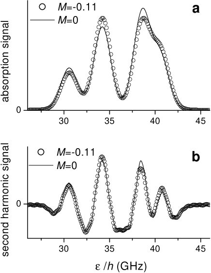
Figure 28: a : Experimental recordings of absorption signals obtained at 0.0925 T in pure ${}^{3}\mathrm{He}$ (pressure 8.5 mbar) for $M$=0 (solid line) or in a steady-state OP situation (open symbols). The OP is performed using a laser diode (different from the one used to probe absorption) tuned on the maximum absorption of the ($\sigma_{-},$ C₉) transition. The incident pump power is 30 mW, and the transmitted beam is back reflected once through the cell. Lock-in detection is performed at the modulation frequency $f_{\mathrm{RF}}$ of the RF discharge. b : Experimental recordings of signals obtained with a frequency-modulated probe beam and second-harmonic phase-sensitive detection (see text) in the same conditions.

They are obtained with the same technique as for line intensity measurements (section 3.2.1), using a modulation (at a frequency $f_{\mathrm{RF}}\sim$100 Hz) of the RF discharge excitation of the plasma and a phase-sensitive analysis at $f_{\mathrm{RF}}$ of the transmitted probe intensity. The recorded spectra are quite similar to those of figure 19, but four lines are obtained for this $\pi$ polarisation. A fit of the spectra by a sum of four Gaussian lines is used to obtain the relative line intensities given in table 3.

$\epsilon/h$ (GHz) 30.61 34.24 38.60 40.60 level, $m_{F}$ A₆, + A₅, $-$ A₃, + A₂, $-$ $S_{0}/T_{ij}$ 1.003 0.991 0.989 1.018 $S/T_{ij}$ 0.890 1.098 0.884 1.127 $S/S_{0}$ 0.888 1.109 0.894 1.108 combination $a_{6}/a_{5}$ $a_{6}/a_{2}$ $a_{3}/a_{5}$ $a_{3}/a_{2}$ $M$ for $S_{0}$ 0.006 $-$0.001 $-$0.007 $-$0.014 $M$ for $S$ $-$0.105 $-$0.108 $-$0.117 $-$0.121 $M$ for $S/S_{0}$ $-$0.111 $-$0.107 $-$0.110 $-$0.107

Table 3: Table of normalised relative line intensities $S_{0}/T_{ij}$ and $S/T_{ij}$ obtained from fits of the two recordings of figure 28a. The nuclear polarisation $M$ is computed from ratios of intensities for the four relevant combinations of lines ($m_{F}^{\prime}\neq m_{F}$). From the ratios $S/S_{0}$ (last line), the nuclear polarisation is deduced to be $M$=$-$0.109$\pm$0.002. This negative polarisations is obtained due to the use of $\sigma_{-}$ OP light.

As for the absorption measurements discussed in section 3.2.2, several systematic effects actually limit the accuracy of the measurements of relative line intensities (e.g. imperfect light polarisation or ${}^{3}\mathrm{He}$ purity). A $\pm$1.5 % deviation from the computed intensity ratios is observed for the $M$=0 recording in figure 19 (first line in table 3). This accounts for the observed scatter in the determinations of $M$ deduced from the ratios of signal amplitudes (“$M$ for $S$” values in table 3), and justifies the use of the absorption measurements at null polarisation and of equation 53 to actually compute $M$ (last line in table 3).

Replacing a continuous frequency scan by operation at two fixed frequencies requires accurate independent settings of the laser frequencies to probe the centres of the absorption lines. With a different modulation scheme, in which the laser frequency is modulated over a small fraction of the Doppler width at a frequency $f_{\mathrm{probe}}\sim$1 kHz, a phase-sensitive analysis at $f_{\mathrm{probe}}$ of the transmitted probe intensity provides an error signal proportional to the derivative of the absorption signal. This error signal allows to lock the laser frequency on any absorption line. A second harmonic phase-sensitive analysis (at $2f_{\mathrm{probe}}$) provides a signal proportional to the second derivative of the absorption signal. This is displayed in figure 28b for the same conditions as those of the absorption measurement in figure 28a. The four transitions appear to be better resolved, and the amplitude variations can similarly be used to deduce the polarisation $M$. The respective advantages of the two modulation schemes will be discussed in the next section.

In isotopic mixtures the same transitions could still be probed, but the overlap of the intense ${}^{4}\mathrm{He}$ lines precludes any reliable analysis of the C₉ transition. Instead we present recordings of absorption spectra on the D₀ lines in figure 29 for a transverse probe beam with equal weights on $\sigma$ and $\pi$ polarisations.

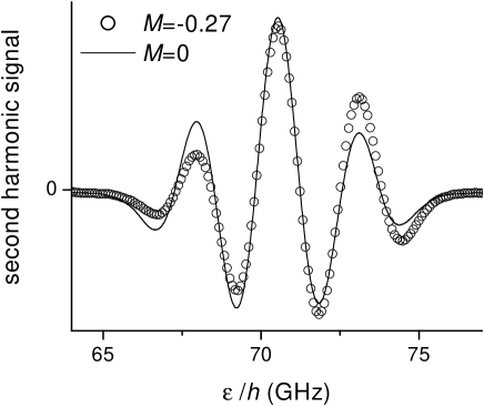
Figure 29: Experimental recordings of absorption signals 0.0925 T in an isotopic mixture ($R$=3, total pressure 8.5 mbar) for $M$=0 (solid line) or in a steady-state OP situation (open symbols). $\sigma$ and $\pi$ polarisations are equally present in the transverse probe beam. The OP is performed in the same way as for the recordings in figure 28 but on the ($\sigma_{-},$ D₀) transition.

While the same laser power is used for OP, a much larger nuclear polarisation ($M$=0.27) is deduced from this measurement in an isotopic mixture. This higher efficiency is similar to that systematically observed in low field OP experiments Stoltz , and is related to the more efficient absorption of the pumping light by the ($\sigma_{-}$,D₀) line.

Frequency scans over 20 GHz as displayed in figures 28 and 29 are performed in $\sim$100 s and can be used only to characterise steady-state situations. A simple method to track the dynamics of buildup or decay of $M$ in an OP experiment consists in actually repeating identical experiments with the probe laser frequency tuned to different transitions. The result of the analysis of two successively performed absorption recordings is given in figure 30.

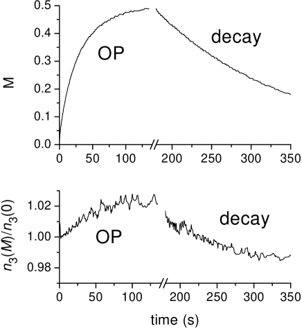
Figure 30: Nuclear polarisation $M$ and relative changes in total metastable density $n_{3}$ deduced from successive measurements of absorption signals by states A₅ and A₃ ($B$=0.0925 T, ${}^{3}\mathrm{He}$ pressure 1.07 mbar). The OP is performed on the ($\sigma_{+},$ C₉) transition with 150 mW of incident pumping power starting from an unpolarised gas (this sets the initial time $t$=0). The pumping beam is blocked after 180 s and $M$ exponentially decays back to 0 ($T_{1}$=156 s). Here polarisation is positive due to the choice of $\sigma_{+}$ OP light.

The probed lines in these measurements are the two most intense lines in figure 28a. The recorded signals are obtained with a standard modulation of the RF discharge excitation and a phase-sensitive analysis at $f_{\mathrm{RF}}$ of the transmitted probe intensity. A higher nuclear polarisation is obtained here for two reasons: the gas pressure is lower, and a fibre amplifier is used to increase the pumping beam power Chernikov .

Small changes of the number density $n_{3}$ are derived from the recordings. They result in part from a slow drift in the RF discharge conditions, since in the analysis $n_{3}(0)$ is obtained from the absorptions measured for the $M$=0 situations at the beginning of the recordings. This drift accounts for the $\sim$1 % difference observed over the total duration of the recordings ($>$700 s). Another part ($\sim$2 %) of the change of $n_{3}$ in figure 30 is clearly correlated to the value of the nuclear polarisation. It is known that the electronic orientation in the $2^{3}\mathrm{S}$ state has an influence on the rate of ionising collisions in the plasma:

$$\begin{array}[c]{ccccccccc}\mathrm{He}^{\mathrm{\ast}}&+&\mathrm{He}^{\mathrm{\ast}}&\rightarrow&\mathrm{He}&+&\mathrm{He}^{\mathrm{+}}&+&\mathrm{e}^{\mathrm{-}}\end{array}$$ (56)

(which would ultimately be forbidden in a fully polarised system Schearer70 ). Such an effect probably explains the systematically observed variations of $n_{3}$ with $M$ (here a small increase). However these variations (even their sign) strongly depend on the RF discharge intensity Bigelow92 and are thus difficult to quantitatively predict. This makes the simultaneous measurements of $M$ and $n_{3}$ of special interest for an accurate characterisation of OP kinetics.

3.3.3 Discussion

The frequency scans in figures 28a and 28b illustrate the difference arising from the chosen absorption measurement method: modulation of the RF discharge intensity and detection at $f_{\mathrm{RF}}$, or modulation of the probe frequency and detection at $2f_{\mathrm{probe}}$. The signal-to-noise ratio of the phase-sensitive detection at $f_{\mathrm{RF}}$ is observed to be higher when both amplitudes of the modulations are optimally set. Detection at $f_{\mathrm{RF}}$ may hence be preferred, but this choice is not mandatory (a fair enough signal-to-noise ratio can be obtained, e.g. in figure 29).

Whatever the chosen detection scheme, a modulation of the probe frequency may be applied to obtain a frequency error signal from a phase-sensitive detection at $f_{\mathrm{probe}}$. This allows to precisely adjust the probe frequency on the centre of isolated absorption lines, but is affected by the presence of any neighbouring lines (the effect depends on their distance and relative intensity). Whenever ill-resolved lines are probed to deduce relative populations of individual states, a careful analysis must be performed and appropriate corrections must be applied to the measured signals. These corrections are usually smaller for signals detected at $2f_{\mathrm{probe}}$ when the distance to the nearest line is smaller than the Doppler width $\Delta.$ Conversely, smaller corrections are required for a detection at $f_{\mathrm{RF}}$ if this distance is larger than 1.3$\Delta,$ as is the case for the C₉ doublet in Figure 28 (the exact crossover distance depends on the relative amplitude of the perturbing line). This may seem surprising since ill-resolved lines have narrower features with a detection at $2f_{\mathrm{probe}}$. However it is only the central part of the second derivative of a Gaussian profile which appears to be narrower than the profile itself. Side lobes actually extend beyond the Doppler width, and as a result there may be a significant crosstalk between apparently resolved lines. Indeed, the choice of a detection scheme impacts both on the data analysis and on the accuracy of the results only when measurements at two fixed frequencies are performed: for a complete frequency scan of a set of lines, integration of signals obtained by a detection at $2f_{\mathrm{probe}}$ can be used to exactly reconstruct the usual absorption spectra.

We have tested several methods to obtain time-resolved results with dual-frequency operation of the probe laser. The one used for the recordings in figure 30, which consists in repeating once every measurement, is very simple to implement but is time consuming. However, since the measured values of the atomic density $n_{3}$ and $n_{4}$ usually vary very little with the polarisation, one may alternatively neglect this variation and only perform one absorption measurement. Using equation 54 or 55 with its left-hand site set to 1, the spin-temperature (and hence $M$) can then be obtained from this single absorption measurement. For the measurement of figure 30, this approximation would have resulted in a maximum relative error of 2 % on $M$ and 1 % on the decay rate $T_{1}$.

For situations where very accurate measurements are required, or where the plasma conditions and hence $n_{3}$ and $n_{4}$ may substantially change in the course of an experiment, alternating operation of the probe laser on two frequencies can be obtained by two techniques. A temperature change of the DBR diode can be used to induce the required frequency change (see section 3.1.1), with a typical response time is of order 0.1 s. Following a frequency change of a few GHz, the frequency is actually sufficiently stable to provide a meaningful absorption signal after $\sim$1 s of dead time. This means that the period of the probe frequency changes cannot be shorter that a few seconds, and that the technique is not suitable to measure fast pumping transients of the kind obtained using powerful pumping lasers hypint . A change of the current in the DBR diode can also be used to induce the required frequency change. This is best done at a high enough frequency for the temperature of the device to remain constant ($>$1 kHz), and very fast OP transients can be monitored with this technique. However, the current changes also drive significant power changes of the probe beam. The full elimination of this effect in the absorption measurements requires a careful signal acquisition and analysis, and the absolute accuracy of the results is somewhat reduced compared to the previous techniques.

We finally come back to the initial assumption made in this section, namely that relaxation and OP processes do not affect the ME-ruled distribution of populations in the $2^{3}\mathrm{S}$ state, and discuss their perturbing influence on the optical absorption measurements.

Relaxation of the spin variables in the $2^{3}\mathrm{S}$ state would drive the spin distribution to its true thermal (Boltzmann) equilibrium in the applied field in the absence of ME collisions. Even for $B$=1.5 T and for electronic spins, this equilibrium corresponds to a small polarisation ($\leq$1 %) compared to $M$, so that the effect of relaxation is to reduce the orientation in the probed $2^{3}\mathrm{S}$ state. This leads to under-estimating the true value of the ground state nuclear polarisation with absorption-based optical measurements.

Conversely, OP with an intense pump laser results in an overpolarisation of the pumped $2^{3}\mathrm{S}$ atoms with respect to the spin temperature population distribution (this is the driving process which actually transfers angular momentum to the ground state reservoir of atoms through ME collisions). We have indeed demonstrated in section 3.2.4 that even a moderate laser intensity can induce strong deviations from equilibrium of the population distributions in high magnetic field. However this overpolarisation is a local effect which can simply be measured, and eliminated by displacing the probe beam so as not to overlap the pump beam. Figure 30 clearly shows that blocking the pumping beam to let the nuclear polarisation decay does not change the measured relative populations nor the inferred value for $M$.

Experimentally, the effects of relaxation and OP which we have observed at $B$=0.0925 T are similar to those observed in low field Bigelow92 , and do not significantly affect our optical measurement technique. This remains to be quantitatively assessed in higher fields and at higher pressures, for which hyperfine decoupling and additional relaxation processes might decrease the efficacy of ME collisions to impose a single spin temperature for all populations. Still, based on our systematic study of OP effects up to 1.5 T, we believe that an absorption measurement technique can provide reliable results, especially if one probes the atomic states least sensitive to OP effects, and thus most efficiently coupled to the ground state polarisation (the ${}^{3}\mathrm{He}$ $2^{3}\mathrm{S}$ states $\mathrm{A}_{+}^{l}$ and $\mathrm{A}_{-}^{h}$, as shown in figure 9).

4 Prospects

From a theoretical point of view, we have developed and tested convenient tools to numerically obtain the eigenstates of the $2^{3}\mathrm{S}$ and $2^{3}\mathrm{P}$ levels in ${}^{3}\mathrm{He}$ and ${}^{4}\mathrm{He}$ and explore the characteristic features of the 1083 nm transition in an arbitrary magnetic field. We have also extended the quantitative treatment of ME collisions by deriving rate equations for populations of all sublevels of the $2^{3}\mathrm{S}$ state which are valid for isotopic mixtures in an arbitrary magnetic field. The use of an elementary OP model for the case $M$=0 led to quantitative predictions which have been accurately verified experimentally. A more elaborate OP model, similar to the one introduced for pure ${}^{3}\mathrm{He}$ in low field Nacher85 , can now be developed. This work is in progress, based on the rate equations describing the effects of ME collisions and absorption / emission of light which we have obtained and on an adequate phenomenological treatment of relaxation phenomena.

Experimentally, we have demonstrated that the use of a DBR laser diode and of simple techniques based on standard or Doppler-free absorption measurement can provide a wealth of spectroscopic information on the 1083 nm transition in helium up to high magnetic fields.

Saturated absorption experiments (or velocity-selective OP measurements) have been performed in this work only as a means to perform Doppler-free measurement of transition frequencies, to check for the soundness of our experimental techniques. However the complex signals which we have obtained, combining narrow lines and broad pedestals, also provide quantitative information on collisional redistribution of orientation between atoms of different velocity classes in the $2^{3}\mathrm{S}$ state. These collisions are a key process when OP is performed at high pumping intensity and saturation effects are important hypint . A detailed study is currently being made using independent pump and probe laser frequencies to fully characterise the collisional transfer of orientation and the saturation effects. This work will also provide useful guidance for designing improved laser sources for high power OP.

A detailed study of several systematic effects on absorption measurements has allowed us to assess the accuracy of relative population measurements in various situations. It could be expected that hyperfine decoupling would hamper angular momentum transfer by ME collisions at very high field. We have demonstrated that ME collisions actually have a very different efficacy for coupling populations in the $2^{3}\mathrm{S}$ state to the nuclear polarisation in the ground state depending on the value of the magnetic field, the helium isotope and the implied $2^{3}\mathrm{S}$ state sublevel. Based on these techniques and results, and using the optical measurement methods described in the last section of this article, a systematic study of OP of helium in non-standard conditions (high magnetic field, high pressure) can now be performed. One of the motivations of this study is the observation, mentioned in the introduction, that higher nuclear polarisations may be obtained by applying a stronger field (0.1 T) than usual. We believe that a systematic study will help to elucidate the nature of relaxation processes in the plasma, and may lead to reduce their effect in situations of practical interest for applications requiring hyperpolarised ${}^{3}\mathrm{He}$ .

Appendix: tables and matrices

The tables and matrices used in the body of the text are collected in this Appendix.

Fine-structure term parameters

are listed in tables 4 and 5:

$2^{3}\mathrm{P}_{\mathrm{0}}$ $2^{3}\mathrm{P}_{\mathrm{1}}$ $2^{3}\mathrm{P}_{\mathrm{2}}$ $2^{1}\mathrm{P}$ $2^{3}\mathrm{P}_{\mathrm{0}}$ $E_{0}$ 0 0 $2^{3}\mathrm{P}_{\mathrm{1}}$ 0 $E_{1}$ 0 $2^{3}\mathrm{P}_{\mathrm{2}}$ 0 0 $E_{2}$ $2^{3}\mathrm{P}_{\mathrm{0}}$ $E_{0}$ 0 0 0 $2^{3}\mathrm{P}_{\mathrm{1}}$ 0 $E_{1}^{\prime}$ 0 $E_{M}$ $2^{3}\mathrm{P}_{\mathrm{2}}$ 0 0 $E_{2}$ 0 $2^{1}\mathrm{P}$ 0 $E_{M}$ 0 $\Delta$

Table 4: $m_{J}$-independent matrix elements of the fine-structure term $H_{fs}$ in the $\left\{\left|J;m_{J}\right\rangle\right\}$ basis, used to compute the $2^{3}\mathrm{P}$ state structure. $E_{0},$ $E_{1},$ $E_{2}$ are the true energies of the $2^{3}\mathrm{P}_{0,1,2}$ levels in zero $B$ field. The last 4 lines of the table provide the expression of the effective Hamiltonian explicitly considering the $2^{1}\mathrm{P}$—$2^{3}\mathrm{P}$ mixing, with additional parameters $\Delta,$ $E_{M}$ and $E_{1}^{\prime}.$

${}^{4}\mathrm{He}$ (MHz) ${}^{3}\mathrm{He}$ (MHz) reference $E_{2}$ 0 0 $E_{1}$ 2291.175 2291.926 Storry00 ; Castillega00 $E_{0}$ 29616.950 29616.675 Minardi99 $\Delta$ 6.1423$\times$10⁷ 6.1431$\times$10⁷ Hinds85 $E_{M}$ -17035 -17037 Hinds85 $E_{1}^{\prime}$ 2295.899 2296.651 see caption

Table 5: Values of the energies for ${}^{4}\mathrm{He}$ and ${}^{3}\mathrm{He}$ are given with reference to that of the $2^{3}\mathrm{P}_{2}$ level of each isotope. We use the most recent and accurate values whenever possible, and mass effects are evaluated as corrections Hinds85 ; Hijikata88 . $E_{1}$ and $E_{1}^{\prime}$ are almost exactly 1 MHz larger, and $E_{M}$ 1000 times larger, than the values of reference Hinds85 , probably due to misprints in the article. $E_{1}^{\prime}$ is not a free parameter since the eigenvalue $E_{1}$ must be obtained. It is given by $E_{1}^{\prime}=E_{1}+E_{M}^{2}/\left(\Delta-E_{1}\right).$

The Zeeman Hamiltonian,

including relativistic corrections of $O\left(\alpha^{2}\right),$ consists of a linear term $H_{1}$ and a quadratic term $H_{2}.$ The linear term contains a correction with respect to the simple expression in equations 1 and 5:

$$H_{1}=H_{Z}+\mu_{B}g_{x}\left(SO^{(2)}\right)\cdot B,$$ (A1)

in which the tensor operator $O^{(2)}$ involves $L$ Lhuillier76 ; Yan94 ; Lewis70 . Due to this additional term, $H_{1}$ is more easily expressed in the coupled $\left|J,m_{J}\right\rangle$ basis, as is the quadratic term $H_{2}.$ $H_{1}$+$H_{2}$ has non-zero elements only between sublevels of equal $m_{J},$ which involve five different $g$-factors in the $2^{3}\mathrm{P}$ state, and two in the $2^{3}\mathrm{S}$ state, all listed in table III of Yan94 . In the present work, this full expression is used only to evaluate the error resulting from neglected terms involving $g_{x}$ and $H_{2}$. The values listed in table 6 which are used for $g_{S}^{\prime}$ and $g_{L}^{\prime}$ are taken from Yan94 , limiting the number of significant digits in order to be consistent with having neglected $g_{x}^{\prime}.$ The mass-dependence of $g_{L}^{\prime}$ is also computed from results of Yan94 , separating out the mass-dependent term:

$$g_{L}=1-\frac{m}{M_{i}}\left\{1+\frac{2F_{1}}{\sqrt{6}}\left(\frac{M_{i}}{M_{4}}-1\right)\right\}+\delta g_{L},$$ (A2)

in which $M_{i}$ stands for the mass of either isotope ($i$=3,4) and $\delta g_{L}$ is the correction for ${}^{4}\mathrm{He}$ given in the reference.

$g_{S}^{\prime}$ $g_{L}^{\prime}\left({}^{4}\mathrm{He}\right)$ $g_{L}^{\prime}\left({}^{3}\mathrm{He}\right)$ $2^{3}\mathrm{S}$ 2.002237319 0 0 $2^{3}\mathrm{P}$ 2.002238838 0.999873626 0.999827935

Table 6: Values of the $g$-factors used in the simplified form of the Zeeman Hamiltonian given in equations 1 and 5. The nuclear term in equation 5 involves $g_{I}$=2.31748$\times$10${}^{-3}.$ The value of the Bohr magneton in frequency units is $\mu_{B}$=13996.242 MHz/T DrakeHB .

The transition matrix elements $T_{m_{S}j}^{(4)}$ and $T_{ij}$

are obtained using the eigenstates of the $2^{3}\mathrm{S}$ and $2^{3}\mathrm{P}$ states and the selection rule operator $T(e_{\lambda})$:

$$T_{m_{S}j}^{(4)} =\left|\left\langle m_{S}\left|T(e_{\lambda})\right|Z_{j}\right\rangle\right|^{2}$$ (A3)

$$T_{ij} =\left|\left\langle A_{i}\left|T(e_{\lambda})\right|B_{j}\right\rangle\right|^{2},$$ (A4)

with matrix elements of $T(e_{\lambda})$ given by:

$$\left\langle m_{S}\left|T(e_{\lambda})\right|m_{S}^{\prime},m_{L}\right\rangle=\delta(m_{S},m_{S}^{\prime})\times\Sigma(e_{\lambda},m_{L})$$ (A5)

for ${}^{4}\mathrm{He}$, and by:

$$\left\langle m_{S}:m_{I}\left|T(e_{\lambda})\right|m_{S}^{\prime},m_{L}:m_{I}^{\prime}\right\rangle=\\ \delta(m_{S},m_{S}^{\prime})\delta(m_{I},m_{I}^{\prime})\times\Sigma(e_{\lambda},m_{L}),$$ (57)

for ${}^{3}\mathrm{He}$, with $\Sigma(e_{\lambda},m_{L})$ as given in table 7.

$m_{L}$=1 $m_{L}$=0 $m_{L}$=-1 $\sigma_{+}$ 1 0 0 $\pi$ 0 1 0 $\sigma_{-}$ 0 0 1

Table 7: Selection rules allow transitions only if angular momentum is conserved, depending on the polarisation state of the light, $e_{\lambda}=\sigma_{+},$ $\sigma_{-}$ or $\pi,$ and on $m_{L}.$

The matrix $F_{6}$

which represents the contact interaction term of the hyperfine Hamiltonian $H_{hfs}$ (equation 6) in the decoupled $\left\{\left|m_{S}:m_{I}\right\rangle\right\}$ basis and the values of the hyperfine coupling constants $A_{\mathrm{S}}$ and $A_{\mathrm{P}}$ for the $2^{3}\mathrm{S}$ and $2^{3}\mathrm{P}$ states respectively are given in table 8:

	$m_{S}:m_{I}$
$m_{S}$:$m_{I}$	$1$:$+$	$0$:$+$	$-1$:$+$	$1$:$-$	$0$:$-$	$-1:-$
$1$:$+$	1/2
$0$:$+$				1/$\sqrt{2}$
$-1$:$+$			-1/2		1/$\sqrt{2}$
$1$:$-$		1/$\sqrt{2}$		-1/2
$0$:$-$			1/$\sqrt{2}$
$-1$:$-$						1/2

Table 8: Matrix elements of $F_{6}/A_{\mathrm{S}}$ (equation 7). Values of the hyperfine coupling constants of equation 6 are $A_{\mathrm{S}}$= $-4493.134$ MHz Rosner70 and $A_{\mathrm{P}}$=$-4283.026$ MHz, 0.019% lower than the value the corresponding parameter $C$ of reference Prestage85 to account for singlet admixture effects (see text).

Computed line positions and intensities

for $B$=0 which are represented in figure 3 are listed in table 9. The results for ${}^{3}\mathrm{He}$ slightly differ from previously published data Nacher85 due to the use of a more accurate Hamiltonian.

	$\epsilon/h$ (GHz)	Intensity
C1	0	0.03566
C2	4.51159	0.37482
C3	4.95920	2
C4	5.18076	1.29767
C5	6.73970	1.29767
C6	11.25129	0.29185
C7	11.92046	0.03566
C8	32.60452	0.29185
C9	39.34422	0.37482
D2	38.53362	5/3
D1	40.82479	1
D0	70.44174	1/3

Table 9: Optical transition energies and intensities for $B$=0. The energies $\epsilon$ are referenced to that of the C₁ transition, the intensities are the partial sums of the transition matrix elements $T_{ij}$ for each line, and obey the total sum rule of equation 10.

The matrix elements $\left\langle J,m_{J}\left|P_{4}\right|m_{L},m_{S}\right\rangle$

of the transformation operator $P_{4}$ from the $\left(L,S\right)$ to the $\left(J\right)$ representation for the $2^{3}\mathrm{P}$ state of ${}^{4}\mathrm{He}$ are given in table 10 . The additional term $H_{hfs}^{cor}$ in equation 6 is given in table 11. It only involves 2 parameters $d$ and $e$, similar to parameters $D/2$ and $E/5$ defined by the Yale group Hinds85 but with values adjusted to effectively take couplings to singlet states into account with this simple model.

	$m_{L},m_{S}$
$J$;$m_{J}$	1,1	0,1	$-$1,1	1,0	0,0	$-$1,0	1,$-$1	0,$-$1	$-$1,$-$1
2;2	1
2;1		1/$\sqrt{2}$		1/$\sqrt{2}$
2;0			1/$\sqrt{6}$		2/$\sqrt{6}$		1/$\sqrt{6}$
2;$-$1						1/$\sqrt{2}$		1/$\sqrt{2}$
2;$-$2									1
1;1		$-$1/$\sqrt{2}$		1/$\sqrt{2}$
1;0			$-$1/$\sqrt{2}$				1/$\sqrt{2}$
1;$-$1						$-$1/$\sqrt{2}$		1/$\sqrt{2}$
0;0			1/$\sqrt{3}$		$-$1/$\sqrt{3}$		1/$\sqrt{3}$

Table 10: Matrix elements of the transformation operator $P_{4}$ (in equation 4). The inverse transformation is given by the transposed matrix : $P_{4}^{-1}\left(i,j\right)$=$P_{4}\left(j,i\right).$

	$m_{L},m_{S}:+$
$m_{L}$,$m_{S}$:$m_{I}$	1,1	0,1	$-$1,1	1,0	0,0	$-$1,0	1,$-$1	0,$-$1	$-$1,$-$1
1,1:+	$d$+2$e$
0,1:+		$-$4$e$		3$e$
$-$1,1:+			$-$$d$+2$e$		$-$3$e$
1,0:+		3$e$		$d$
0,0:+			$-$3$e$		0		3$e$
$-$1,0:+						$-$$d$		$-$3$e$
1,$-$1:+					3$e$		$d$$-$2$e$
0,$-$1:+						$-$3$e$		4$e$
$-$1,$-$1:+									$-$$d$$-$2$e$
1,1:$-$		$\sqrt{2}$($d$+3$e$)		$-$$\sqrt{2}e$
0,1:$-$			$\sqrt{2}$($d$$-$3$e$)		2$\sqrt{2}e$
$-$1,1:$-$						$-$$\sqrt{2}e$
1,0:$-$			6$\sqrt{2}e$		$\sqrt{2}d$		$-$$\sqrt{2}e$
0,0:$-$						$\sqrt{2}d$		2$\sqrt{2}e$
$-$1,0:$-$									$-$$\sqrt{2}e$
1,$-$1:$-$						6$\sqrt{2}e$		$\sqrt{2}$($d$$-$3$e$)
0,$-$1:$-$									$\sqrt{2}$($d$+3$e$)
$-$1,$-$1:$-$

Table 11: Matrix elements of $H_{hfs}^{cor}$ in equation 6. Half of the matrix is explicitely given, the missing elements being obtained using the matrix symmetries with respect to the two diagonals (the same matrix element is obtained when all six signs of angular momentum projections are changed). The values of the parameters are $d$=$-$14.507 MHz and $e$= 1.4861 MHz, slightly larger than the values of the corresponding parameters $D/2$ and $E/5$ of reference Prestage85 (see text).

Given the total Hamiltonian in the $2^{3}\mathrm{S}$ state,

which couples only states $\left|m_{S}:m_{I}\right\rangle$ of given $m_{F}=m_{S}+m_{I},$ a simple analytical expression of the eigenstates and of the energies can be derived. To simplify the following expressions, we introduce the reduced magnetic field $b$ (note that $A_{\mathrm{S}}<0$) and the nuclear correction $\epsilon$:

$$b =-g_{S}^{{}^{\prime}}\mu_{B}B/A_{\mathrm{S}}$$ (A7)

$$\epsilon =g_{I}/2g_{S}^{{}^{\prime}}.$$ (A8)

The $m_{F}=\pm 3/2$ states, $\left|-1:-\right\rangle$ and $\left|1:+\right\rangle,$ are eigenvalues with energies $\left(1/2\pm\beta\left(1+\epsilon\right)\right)A_{\mathrm{S}}.$ In the $m_{F}=+1/2$ subspace, the matrix of the reduced Hamiltonian $H_{6}/A_{\mathrm{S}}$ on the basis $\left\{\left|0:+\right\rangle,\left|1:-\right\rangle\right\}$ is:

$$\left(\begin{array}[c]{cc}-b\epsilon&1/\sqrt{2}\\ 1/\sqrt{2}&\ -b\left(1-\epsilon\right)-1/2\end{array}\right)$$ (A9)

(the matrix for $m_{F}=-1/2$ on the basis $\left\{\left|0:-\right\rangle,\left|-1:+\right\rangle\right\}$ is obtained replacing $\beta$ by -$\beta$ in equation A9). The level energies are:

$$W_{+}^{h,l}=-\frac{A_{\mathrm{S}}}{4}\left(1+2b\right.\\ \pm\sqrt{9+4b+4b^{2}-8b\epsilon-16b^{2}\epsilon\left(1-\epsilon\right)})$$ (58)

$$W_{-}^{h,l}=-\frac{A_{\mathrm{S}}}{4}\left(1-2b\right.\\ \pm\sqrt{9-4b+4b^{2}+8b\epsilon-16b^{2}\epsilon\left(1-\epsilon\right)})\allowbreak,$$ (59)

in which the upper indices $h\$and $l$ refer to the higher and lower energies respectively, and the lower index is the sign of $m_{F}.$ With different notations, these expressions would be identical to those given in reference Prestage85 but for a misprint (a missing factor 1/2 in the last line of their equation 3). Here, both $W_{+}^{h}$ and $W_{-}^{h}$ are obtained for positive sign in the second lines of equations 58 and 59. The field dependence of all energies is shown in figure 2 in the main text. The corresponding eigenstates can be simply written introducing the field-dependent angles $\theta_{+}$ and $\theta_{-}$:

$$\tan\theta_{+} =-\sqrt{2}\left(W_{+}^{h}/A_{\mathrm{S}}+1/2+b\left(1-\epsilon\right)\right)$$ (A12)

$$\tan\theta_{-} =-\sqrt{2}\left(W_{-}^{h}/A_{\mathrm{S}}-b\epsilon\right)$$ (A13)

$$\mathrm{A}_{+}^{h} =-\sin\theta_{+}\left|0:+\right\rangle+\cos\theta_{+}\left|1:-\right\rangle$$ (A14)

$$\mathrm{A}_{+}^{l} =\cos\theta_{+}\left|0:+\right\rangle+\sin\theta_{+}\left|1:-\right\rangle$$ (A15)

$$\mathrm{A}_{-}^{h} =-\sin\theta_{-}\left|-1:+\right\rangle+\cos\theta_{-}\left|0:-\right\rangle$$ (A16)

$$\mathrm{A}_{-}^{l} =\cos\theta_{-}\left|-1:+\right\rangle+\sin\theta_{-}\left|0:-\right\rangle.$$ (A17)

The variation of the angles $\theta_{+}$ and $\theta_{-}$ in shown in figure 31.

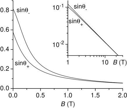
Figure 31: The level-mixing parameters $\sin\theta_{+}$ and $\sin\theta_{-}$ are plotted as a function of the magnetic field $B.$ Insert : asymptotic 1/$B$ decays at high field, with almost equal values of order 1.1$\times$10^-2 at 10 Tesla.

The large amount of state mixing due to hyperfine coupling at low field ($\sin^{2}\theta_{+}$=1/3, $\sin^{2}\theta_{-}$=2/3 for $B$=0) is strongly reduced above 1T ($\sin^{2}\theta_{\pm}\sim 0.012/B^{2}$). Our state naming convention in most of this article ($\mathrm{A}_{1}$ to $\mathrm{A}_{6}$ by increasing energies) introduces three field intervals due to two level crossings. The first crossing occurs at 0.1619 T between $\left|1:+\right\rangle$ and $\mathrm{A}_{-}^{h},$ the second one at 4.716 T between $\mathrm{A}_{-}^{h}$ and $\mathrm{A}_{+}^{l}.$ Altogether, three states are affected by these level crossings, as summarised in table 12.

$B\text{ (T)}$	$<\text{0.1619}$	0.1619–4.716	$>\text{4.716}$	$\text{any }B$
$\mathrm{A}_{1}$				$\left|-1:-\right\rangle$
$\mathrm{A}_{2}$				$\mathrm{A}_{-}^{l}$
$\mathrm{A}_{3}$	$\mathrm{A}_{+}^{l}$	$\mathrm{A}_{+}^{l}$	$\mathrm{A}_{-}^{h}$
$\mathrm{A}_{4}$	$\left|1:+\right\rangle$	$\mathrm{A}_{-}^{h}$	$\mathrm{A}_{+}^{l}$
$\mathrm{A}_{5}$	$\mathrm{A}_{-}^{h}$	$\left|1:+\right\rangle$	$\left|1:+\right\rangle$
$\mathrm{A}_{6}$				$\mathrm{A}_{+}^{h}$

Table 12: Table of correspondence between the state names used in this Appendix and the energy-ordered naming convention $\mathrm{A}_{1}$ to $\mathrm{A}_{6}$.

ME matrices:

we now provide the elements of the $B$-dependent ME matrices $L,$ $G^{4},$ $E^{3},$ $F^{3},$ $E^{4}$ and $F^{4}$ which appear in rate equations 34 to 36. The six relative populations $a_{i}$ of the text are here designated by $a_{--},$ $a_{-}^{l},$ $a_{+}^{l},$ $a_{++},$ $a_{-}^{h},$ $a_{+}^{h}.$ This indexing convention is the same for the state names and the corresponding populations, so that table 12 can be used to transform the indexing, or to determine the permutation of rows and columns required for $B>$0.1619 T between the matrices provided in tables 13 to 17 and those appearing in equations 34 to 36. For more compact expressions, we use the following notations:

$$c_{\pm}=\cos^{2}\theta_{\pm},~{}s_{\pm}=\sin^{2}\theta_{\pm}.$$ (A18)

These matrices are not fully independent. In particular, the steady-state solutions of equations 32 and 33, given in equations 38 and 39, are independent on the isotopic ratio $R.$ Substitution of the steady state solutions $y_{i}={\textstyle\sum_{k}}G_{ik}^{4}a_{k}$ of equation 35 in equation 36 can be used to show that $E^{3}=E^{4}\cdot G^{4}$ and $F^{3}=F^{4}\cdot G^{4},$ two field-independent relations which can be directly verified on the matrices given in tables 14 to 17.

$a_{--}$	$a_{-}^{l}$	$a_{+}^{l}$	$a_{++}$	$a_{-}^{h}$	$a_{+}^{h}$
-1	$c_{-}$-$s_{-}$	$c_{+}$-$s_{+}$	1	$s_{-}$-$c_{-}$	$s_{+}$-$c_{+}$

Table 13: Matrix elements of operator $L$ (equation 34).

	$a_{--}$	$a_{-}^{l}$	$a_{+}^{l}$	$a_{++}$	$a_{-}^{h}$	$a_{+}^{h}$
$y_{1}$	1	$c_{-}$	0	0	$s_{-}$	0
$y_{2}$	0	$s_{-}$	$c_{+}$	0	$c_{-}$	$s_{+}$
$y_{3}$	0	0	$s_{+}$	1	0	$c_{+}$

Table 14: Matrix elements of $G^{4}$ (equation 35).

		2$E^{4}$			2$F^{4}$
	$y_{1}$	$y_{2}$	$y_{3}$	$y_{1}$	$y_{2}$	$y_{3}$
$a_{--}$	1	0	0	-1	0	0
$a_{-}^{l}$	$c_{-}$	$s_{-}$	0	$c_{-}$	-$s_{-}$	0
$a_{+}^{l}$	0	$c_{+}$	$s_{+}$	0	$c_{+}$	-$s_{+}$
$a_{++}$	0	0	1	0	0	1
$a_{-}^{h}$	$s_{-}$	$c_{-}$	0	$s_{-}$	-$c_{-}$	0
$a_{+}^{h}$	0	$s_{+}$	$c_{+}$	0	$s_{+}$	-$c_{+}$

Table 15: Matrix elements of 2$E^{4}$ and 2$F^{4}$ (twice those of $E^{4}$ and $F^{4}$ in equation 36).

	$a_{--}$	$a_{-}^{l}$	$a_{+}^{l}$	$a_{++}$	$a_{-}^{h}$	$a_{+}^{h}$
$a_{--}$	1	$c_{-}$	0	0	$s_{-}$	0
$a_{-}^{l}$	$c_{-}$	$c_{-}^{2}$+$s_{-}^{2}$	$c_{+}s_{-}$	0	2$c_{-}s_{-}$	$s_{+}s_{-}$
$a_{+}^{l}$	0	$c_{+}s_{-}$	$c_{+}^{2}$+$s_{+}^{2}$	$s_{+}$	$c_{+}c_{-}$	2$c_{+}s_{+}$
$a_{++}$	0	0	$s_{+}$	1	0	$c_{+}$
$a_{-}^{h}$	$s_{-}$	2$c_{-}s_{-}$	$c_{+}c_{-}$	0	$c_{-}^{2}$+$s_{-}^{2}$	$c_{-}s_{+}$
$a_{+}^{h}$	0	$s_{+}s_{-}$	2$c_{+}s_{+}$	$c_{+}$	$c_{-}s_{+}$	$c_{+}^{2}$+$s_{+}^{2}$

Table 16: Matrix elements of 2$E^{3}$ (twice those of $E^{3}$ in equation 36).

	$a_{--}$	$a_{-}^{l}$	$a_{+}^{l}$	$a_{++}$	$a_{-}^{h}$	$a_{+}^{h}$
$a_{--}$	-1	-$c_{-}$	0	0	-$s_{-}$	0
$a_{-}^{l}$	$c_{-}$	$c_{-}^{2}$-$s_{-}^{2}$	-$c_{+}s_{-}$	0	0	-$s_{+}s_{-}$
$a_{+}^{l}$	0	$c_{+}s_{-}$	$c_{+}^{2}$-$s_{+}^{2}$	-$s_{+}$	$c_{+}c_{-}$	0
$a_{++}$	0	0	$s_{+}$	1	0	$c_{+}$
$a_{-}^{h}$	$s_{-}$	0	-$c_{+}c_{-}$	0	$s_{-}^{2}$-$c_{-}^{2}$	-$c_{-}s_{+}$
$a_{+}^{h}$	0	$s_{+}s_{-}$	0	-$c_{+}$	$c_{-}s_{+}$	$s_{+}^{2}$-$c_{+}^{2}$

Table 17: Matrix elements of 2$F^{3}$ (twice those of $F^{3}$ in equation 36).

References

- (1) D. Rohe et al., Phys. Rev. Lett. 83 (1999) 4257.
- (2) J. Becker et al., Nuc. Instr. & Meth. A 402 (1998) 327.
- (3) G.L. Jones et al., Nuc. Instr. & Meth. A 440 (2000) 772.
- (4) G. Tastevin, Physica Scripta T86 (2000) 46.
- (5) T. Chupp and S. Swanson, Adv. At. Mol. Opt. Phys. 45 (2001) 51.
- (6) F.D. Colegrove, L.D. Schearer and G.K. Walters, Phys. Rev. 132 (1963) 2561.
- (7) P.-J. Nacher and M. Leduc, J. Phys. Paris 46 (1985) 2057.
- (8) N.P. Bigelow, P.J. Nacher and M. Leduc, J. Phys. II France 2 (1992) 2159.
- (9) M Leduc, S.B. Crampton, P.J. Nacher and F. Laloë, Nuclear Sci. App. 1 (1983) 1.
- (10) J. Becker et al., Nucl. Instr. and Meth. A 346 (1994) 45.
- (11) P.-J. Nacher, G. Tastevin, X. Maitre, X. Dollat, B. Lemaire and J. Olejnik, Eur. Radiol. 9 (1999) B18.
- (12) T. R. Gentile et al., Magn. Reson. Med. 43 (2000) 290.
- (13) L. Darrasse et al. in: Proc. Int. Soc. for Mag. Res. in Medicine, Sydney (1998) 449.
- (14) J.L. Flowers, B.W. Petley and M.G. Richards, J. Phys. B 23 (1990) 1359.
- (15) J.L. Flowers, C.J. Bickley, P.W. Josephs-Franks and B.W. Petley, IEEE Trans. Instrum. Meas. 46 (1997) 104.
- (16) E. Courtade, F. Marion, P.J. Nacher, G. Tastevin, T. Dohnalik and K. Kiersnowski, Hyperfine Interactions 127 (2000) 451.
- (17) M. Pavlovic and F. Laloë, J. Phys. France 31 (1970) 173.
- (18) W.A. Fitzsimmons, N.F. Lane and G.K. Walters, Phys. Rev. A 19 (1968) 193.
- (19) R. Chapman and M. Bloom, Canad. J. Phys. 54 (1976) 861.
- (20) R. Barbé, PhD Thesis (1977) Paris.
- (21) P.-J. Nacher, PhD Thesis (1985) Paris.
- (22) E. Courtade, PhD Thesis (2001) Paris.
- (23) E. Courtade, P.-J. Nacher, C. Dedonder, C. Jouvet and T. Dohnalik, in preparation.
- (24) W.D. Philips and H. Metcalf, Phys. Rev. Lett. 48 (1982) 596.
- (25) A. Robert et al., Science 292 (2001) 461.
- (26) F. Pereira Dos Santos et al., Phys. Rev. Lett. 86 (2001) 3459.
- (27) C.H. Storry, M.C. George and E.A. Hessels, Phys. Rev. Lett. 84 (2000) 3274.
- (28) J. Castillega, D. Livingstone, A. Sanders and D. Shiner, Phys. Rev. Lett. 84 (2000) 4321.
- (29) D. Shiner, R. Dixson and V. Vedantham, Phys. Rev. Lett. 74 (1995) 3553.
- (30) C. Lhuillier, J.-P. Faroux and N. Billy, J. Physique 37 (1976) 335.
- (31) D.-H. Yang, P. McNicholl and H. Metcalf, Phys. Rev. A 33 (1986) 1725.
- (32) Z.-C. Yan and G.W.F. Drake, Phys. Rev A 50 (1994) R1980.
- (33) A. Kponou et al., Phys. Rev. A 24 (1981) 264 ; W. Frieze et al, ibid., 279.
- (34) J.D. Prestage, C.E. Johnson, E.A. Hinds and F.M.J. Pichanick, Phys. Rev. A.32 (1985) 2712.
- (35) I. Gonzalo and E. Santos, Phys. Rev. A 56 (1997) 3576.
- (36) E.A. Hinds, J.D. Prestage and F.M.J. Pichanick, Phys. Rev. A 32 (1985) 2615.
- (37) K. Hijikata and K. Ohtsuki, J. Phys. Soc. Jap. 57 (1988) 4141.
- (38) Atomic transition probabilities, W.L. Wiese, M.W. Smith and B.M. Glennon, National Standard Reference Data Series NBS 4 (1966).
- (39) Atomic, molecular, and optical physics handbook (AIP Press, G.W.F. Drake ed., 1996).
- (40) D. Bloch, G. Trenec and M. Leduc, J. Phys. B: At. Mol. Phys. 18 (1985) 1093.
- (41) See for instance W.H. Press et al., Numerical recipes in Fortran (Cambridge University Press, 1992) 460.
- (42) Source files or executable programs may be provided on request by one of the authors (P.-J. N.).
- (43) S.A. Lewis, F.M.J. Pichanick and V.W. Hughes, Phys. Rev. A 1 (1970) 86.
- (44) R.B. Partridge and G.W. Series, Proc. Phys. Soc. 88 (1966) 983.
- (45) J. Dupont-Roc, M. Leduc and F. Laloe, J. Physique 34 (1973) 961 and 977.
- (46) M. Pinard and F. Laloë, J. Physique 41 (1980) 799.
- (47) L.W. Anderson, F.M. Pipkin and J.C. Baird, Phys. Rev. 116 (1959) 87.
- (48) W. Happer, Rev. Mod. Phys. 44 (1972) 169.
- (49) J. Dupont-Roc, M. Leduc and F. Laloë, Phys. Rev. Lett. 27 (1971) 467.
- (50) C. Larat, PhD Thesis (1991) Paris.
- (51) F. Minardi et al., Phys. Rev. Lett. 82 (1999) 1112.
- (52) D. Shiner, R. Dixson and P. Zhao, Phys. Rev. Lett. 72 (1994) 1802.
- (53) M. Prevedelli, P. Cancio, G. Giusfredi, F.S. Pavone and M. Inguscio, Optics Commun. 125 (1996) 231.
- (54) This magnet is part of the GE Signa MRI system of the Centre Inter Etablissements de Résonance Magnétique in the Kremlin-Bicêtre hospital. We wish to thank J. Bittoun and his team for providing the opportunity to perform these high-field measurements.
- (55) E. Stoltz, M. Meyerhoff, N. Bigelow, M. Leduc, P.-J. Nacher and G. Tastevin, Appl. Phys. B63 (1996) 629.
- (56) R.C. Greenhow, Phys. Rev. 126 (1964) A660.
- (57) J.M. Daniels and R.S. Timsit, Can. J. Phys. 49 (1971) 539; R.S. Timsit and J.M. Daniels, Can. J. Phys. 49 (1971) 545.
- (58) S.V. Chernikov, J.R. Taylor, N.S. Platonov, V.P. Gaponstev, P.-J. Nacher, G. Tastevin, M. Leduc and M.J. Barlow, Electronics Lett. 33 (1997) 787.
- (59) L.D. Schearer and L.A. Riseberg, Phys. Lett. 33A (1970) 325.
- (60) M. Leduc, P.J. Nacher, G. Tastevin and E. Courtade, Hyperfine Interactions 127 (2000) 443.
- (61) S.D. Rosner and F.M. Pipkin, Phys. Rev. A 1 (1970) 571.