Non-invasive single-bunch matching and emittance monitor

Abstract

On-line monitoring of beam quality for high brightness beams is only possible using non-invasive instruments. For matching measurements, very few such instruments are available. One candidate is a quadrupole pick-up. Therefore, a new type of quadrupole pick-up has been developed for the 26 GeV Proton Synchrotron (PS) at CERN, and a measurement system consisting of two such pick-ups is now installed in this accelerator. Using the information from these pick-ups, it is possible to determine both injection matching and emittance in the horizontal and vertical planes, for each bunch separately. This paper presents the measurement method and some of the results from the first year of use, as well as comparisons with other measurement methods.

I Introduction and background

A quadrupole pick-up is a non-invasive device that measures the quadrupole moment

$$\kappa=\sigma^{2}_{x}-\sigma^{2}_{y}+\bar{x}^{2}-\bar{y}^{2}.$$ (1)

of the transverse beam distribution. Here, $\sigma_{x}$ and $\sigma_{y}$ are the r.m.s. beam dimensions in the horizontal and vertical directions, while $\bar{x}$ and $\bar{y}$ denote the beam position.

The practical use of quadrupole pick-ups was pioneered at SLACMiller et al. (1983), where six such pick-ups, distributed along the linac, were used. The emittance and Twiss parameters of a passing bunch were obtained from the pick-up measurements by solving a matrix equation, derived from the known transfer matrices between pick-ups.

In rings, the use of quadrupole pick-ups has largely focused on the frequency content of the raw signal. Beam width oscillations produce sidebands to the revolution frequency harmonics in the quadrupole signal, at a distance of twice the betatron frequency, and this can be used to detect injection mismatch. This was done at the CERN Antiproton Accumulator, where the phase and amplitude of the detected sidebands were also used to find a proper correction, using an empirical response matrixChohan et al. (1990). However, this measurement was complicated by the fact that the same sidebands can be produced by position oscillations, which demanded that position oscillations were kept very small.

In this paper, the idea behind the SLAC method is applied and further developed for use in rings. The quadrupole pick-ups used for the measurements presented here were specially developed for the CERN PS and optimized to measure the quadrupole momentJansson and Williams (2002).

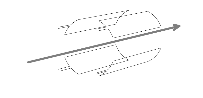
Figure 1: Location of the induction loops. The arrow symbolises the beam. For a centered, round beam no flux passes thru the loop and therefore no signal is induced. Therefore, the quadrupole signal due to beam ellipticity is easy to detect.

They consist of four induction loops oriented to be sensitive to the magnetic flux in the radial direction (see FIG. 1). Since the field from a centered round beam has a flux only in the azimuthal direction, only deviations from roundness or position induce a signal in the loops. Therefore each loop is directly sensitive to the quadrupole moment, unlike previous instruments where the quadrupole moment was extracted by detecting tiny differences between four large electrode signals.

Two pick-ups have been installed in consecutive straight sections of the machineJansson et al. (2001). The optical parameters at their locations are given in TABLE 1. As shown later, it is crucial that the pick-ups be installed at locations with different ratios between horizontal and vertical beta value. The phase advance between pick-ups is also an important input parameter in the data analysis. In order to minimize the dependence of this phase advance on the programmed machine tunes and the beam intensity (space charge detuning), the pick-ups were installed as close as possible to each other.

Table 1: Beta function values and horizontal dispersion at the pick-up locations. The horizontal and vertical phase advances between the two locations are also given. The pick-ups are installed in consecutive straight sections of the PS machine.

Name	$\beta_{x}$	$\beta_{y}$	$D_{x}$	$\Delta\mu_{x}$	$\Delta\mu_{y}$
QPU 03	22.0 m	12.5 m	3.04 m	0.365	0.368
QPU 04	12.6 m	21.9 m	2.30 m

The PS pick-ups provide both beam position and quadrupole moment information, with bunch-by-bunch resolution, over several hundred turns. Since the beam position is also measured, its contribution to the quadrupole moment can be subtracted, leaving only the beam-size related part, $\sigma_{x}^{2}-\sigma_{y}^{2}$. Throughout the rest of this paper, when referring to $\kappa$, it will be assumed that this ‘artificial centering’ has been performed, unless stated otherwise.

Figure 2: Quadrupole moment $\kappa$ measured with a PS pick-up immediately after injection, with and without correction for beam position. The initial beam-size oscillation is clearly visible in the corrected signal. Note the fast decoherence of beam size oscillations, due to direct space charge.

An example of a position-corrected measurement is shown in FIG. 2, where the usefulness of the correction is clear. The initial beam size oscillation due to injection mismatch is clearly visible in the corrected signal. Note that beam-size oscillations are sensitive to the direct space charge, which means that they have a larger tune-spread, and therefore decohere much faster than beam position oscillations. The difference in decoherence time between beam size and position oscillations is therefore a rather direct measure of the incoherent tune shift. The detuning of the quadrupole signal frequencies can also be used to measure the incoherent tune shift, as has been done in the Low Energy Antiproton Ring (LEAR) at CERNChanel (1996).

II Signal Acquisition and treatment

At the input to the data acquisition system, located in a building next to the machine, the analogue signals from the pick-up have the form

$$\Xi(t) = Z_{\Xi}\;\kappa(t-t_{\Xi})\;i(t-t_{\Xi})\quad\;\;\text{quad. moment}$$ (2)

$$\Delta_{x}(t) = Z_{\Delta}\;\bar{x}(t-t_{\Delta_{x}})\;i(t-t_{\Delta_{x}})\quad\text{hor. position}$$ (3)

$$\Delta_{y}(t) = Z_{\Delta}\;\bar{y}(t-t_{\Delta_{y}})\;i(t-t_{\Delta_{y}})\quad\text{ver. position}$$ (4)

where the $Z$s are the transfer impedances, $\kappa$, $\bar{x}$ and $\bar{y}$ are defined as before, and $i$ is the beam current. In the PS, the beam current is not measured by the pick-up itself, so a separate beam current reference signal

$$\Sigma(t)=Z_{\Sigma}\;i(t-t_{\Sigma})\quad\text{sum signal}$$ (5)

is taken from a nearby wall-current monitor. These analogue signals are sampled by digital oscilloscopes. The digitized signals are then re-sampled to correct for the signal timing differences $t_{\Xi}$, $t_{\Delta_{x}}$, $t_{\Delta_{x}}$ and $t_{\Sigma}$. These are mainly due to cable length differences, and have been measured both with a synthetic signal and using the beam.

The analysis of the data is made in a LabView program. In order to resolve single bunches, the data is treated in the time domain, considering each bunch passage separately. The first step in the analysis is to rid the signal of its intensity dependence, by normalizing to the measured beam current. The analysis is performed in two different ways, depending on whether the position and quadrupole moment are expected to be constant or varying along the bunch.

II.1 Position and size constant along bunch

If there is no variation in position and size along the bunch, and one assumes that the quadrupole pick-up and the wall current monitor have the same frequency response, then the shape a given pulse must be exactly the same in all signals (apart from a baseline offset and noise effects). The normalization problem then consists in determining the scaling factor between a pulse in the beam current signal and the corresponding pulse on the pick-up outputs.

To do this, time slices of about one RF period centered on the bunch are selected. Each selected slice is a vector of $N$ samples and, under the above assumption, corresponding slices are proportional to each other. The quadrupole moment can therefore be found as the least squares solution to an overdetermined matrix equation, which in the case of the quadrupole signal has the form

$$\begin{pmatrix}\Sigma_{1}&1\\ \Sigma_{2}&1\\ \vdots&\vdots\\ \Sigma_{N}&1\end{pmatrix}\cdot\begin{pmatrix}\kappa\\ c\end{pmatrix}=\frac{Z_{\Sigma}}{Z_{\kappa}}\begin{pmatrix}\Xi_{1}\\ \Xi_{2}\\ \vdots\\ \Xi_{N}\end{pmatrix}.$$ (6)

The constant $c$ depends on the base line difference and is not used. The same calculation is performed for the position signals, and the position contribution to the quadrupole moment is then subtracted.

An attractive feature of this method, apart from noise suppression, is that the base line is automatically, and unambiguously, corrected for. Differences in frequency response of the two instruments could be corrected by filtering the signals, if these responses are known. However, such sophisticated corrections would enhance noise, and are not necessary in the PS.

II.2 Position or size varying along bunch

Sometimes, there can be a variation in oscillation amplitude and phase along the bunch. At injection into the PS, there are two main causes for this

• The injection kicker pulse is not perfectly flat, which causes a variation of initial position along the bunch. The result is a fast position oscillation in those parts of the bunch that did not receive the correct kick.

• If the injected beam is longitudinally mismatched, the mismatched bunch will rotate in the bucket with the synchrotron frequency, causing the bunch length to oscillate. When the bunch is tilted in longitudinal phase space there is a correlation between energy and time, apparent as a variation of the mean energy along the bunch. The degree of correlation varies as the bunch rotates, and at a position with non-zero dispersion this gives rise to a slow head-tail oscillation at twice the synchrotron frequency. Both PS pick-ups are installed in dispersive regions, and are therefore sensitive to this effect.

• There can also be a variation of the beam dimensions along the bunch, as discussed toward the end of this paper.

In these cases, the basic assumption behind the algorithm described in the previous section is no longer valid. In fact, if the position varies along the bunch, any algorithm that calculates the average position and quadrupole moment of the bunch will give an erroneous result. Since

$$<x^{2}>\neq<x>^{2}$$ (7)

one can not simply use the average bunch position in Eq. (1) when correcting for the position. The correction must be done point-by-point along the bunch. For this purpose, a second normalization algorithm is used, which first establishes and subtracts the base line, and then calculates the position

$$x(t)=\frac{Z_{\Sigma}\,}{Z_{\Delta_{x}}}\frac{\Delta_{x}(t)}{\Sigma(t)}$$ (8)

as well as the quadrupole moment in each point. After this correction, an average beam quadrupole moment can be calculated, but it is also possible to study variations of the beam size along the bunch.

Figure 3: Quadrupole moment (uncorrected) versus expected beam position contribution. The squares and circles represent measurements made with the same pick-up on two different beams. The slope of the line is the same in both cases, and is very close to one (0.983).

III Beam-based calibration

III.1 Internal signal consistency

One can take advantage of the position dependence of the quadrupole moment to make a consistency check between the position and quadrupole moment measurement of the pick-up, using data with large beam position oscillations but stable beam size. Since the beam size oscillations damp away much faster than beam position oscillations, such data can easily be obtained at injection by an appropriate trigger delay. A plot of expected versus measured variation of the quadrupole moment with beam position is shown in FIG. 3, showing a good agreement. This test can easily be automated, and is a good indicator of whether the beam position correction works well.

III.2 Comparison with wire-scanners

Figure 4: Comparison between the measured value from the two quadrupole pick-ups and the expected results calculated from the emittances measured with the wire-scanners. The solid line is the ideal case, and the dotted line includes pick-up offsets measured in the lab prior to installation. All possible ways of combining the wire-scanner measurements are displayed. Note that the cases where the two wire-scanner results are inconsistent also are cases with large estimated systematic error.

The standard method for emittance measurement on a circulating beam in the PS is the fast wire-scanner. In order to test the calibration of the pick-ups, measurements were done on several different stable beams, approximately 15 ms after injection. The quadrupole pick-up signal was acquired over 200 machine turns, at the same time as the wire traversed the beam. The comparative measurement was performed on all the operational beams available in the machine, with the exception of the very high intensity beams that saturate the pick-up amplifiers. Thus there was a significant difference in both beam and machine parameters between the different measurements. This was done in an attempt to randomize any systematic errors. The beam parameters are given in TABLE 2, where the different beams have been tagged with their operational names.

Table 2: Parameters of beams used for comparative measurements. Emittances and momentum spread are 2$\sigma$ values.

Name	$\epsilon_{x}$	$\epsilon_{y}$	$\sigma_{\rm p}$	$I_{\rm bunch}$
SFTPRO	19 $\mu$m	12 $\mu$m	2.7 $\times 10^{-3}$	$2.7\times 10^{12}$
AD	25 $\mu$m	9 $\mu$m	2.7 $\times 10^{-3}$	$3.3\times 10^{12}$
LHC	3 $\mu$m	2.5 $\mu$m	2.2 $\times 10^{-3}$	$6.9\times 10^{11}$
EASTA	8 $\mu$m	1.4 $\mu$m	2.5 $\times 10^{-3}$	$1.4\times 10^{11}$
EASTB	7.5 $\mu$m	1.4 $\mu$m	1.6 $\times 10^{-3}$	$8.6\times 10^{10}$
EASTC	12 $\mu$m	3 $\mu$m	2.4 $\times 10^{-3}$	$4.2\times 10^{11}$

The r.m.s. variation in the measured quadrupole moments from turn to turn was of the order of 0.2-0.5 mm², depending on the beam intensity. Assuming that the beam size was perfectly stable, this gives an estimate of the single-turn resolution of the pick-up measurement. Also the wire-scanner measurements were stable, although for some beams there was a systematic disagreement between the two wire-scanners measuring in the same plane.

To compare the two instruments, the emittances measured with the wire-scanners were used to calculate the expected quadrupole moment at the locations of the pick-ups. The momentum spread required for both the wire scanner measurement and the subsequent calculation was obtained by a tomographic analysis of the bunch shapeHancock et al. (1998). The propagated systematic error was estimated on the assumption that the wire-scanner accuracy is 5% in emittance, the beta function at the pick-ups is known to 5%, the dispersion to 10% and the momentum spread to 3% accuracy. These estimates are rather optimistic, but give considerable propagated errors for certain measurement points. For simplicity, possible correlations between errors (e.g. beta function errors at different locations in the machine) were ignored, and all different error sources were added in quadrature. To accentuate the cases with wire-scanner disagreement, each of the four different ways of combining the two horizontal and two vertical wire-scanners was calculated separately and displayed as separate points. The result is shown in FIG. 4.

Overall, the measured data seem to indicate that the offsets are slightly smaller than measured in the lab, which could be explained by the fact that the pick-ups were dismantled in the lab to be moved to the machine. However, the effect is within the error-bar, and no strong conclusion can therefore be made. Moreover, the pick-ups have been dismantled and rebuilt in the lab, without effect on the measured offsets.

The point corresponding to the EASTC beam appears to disagree somewhat in both planes, although the effect is just about within the error-bar. There are a number of possible explanations for this:

• The PS is operated in a time-sharing mode, where a so-called super-cycle containing a certain number (usually 12) of beam cycles is repeated over and over again. At the time of the measurement, the super-cycle contained several instances of the EASTC beam, and it is known from experience that the position within the super-cycle can affect the beam characteristics. For this particular measurement, it is not guaranteed that the measurements with the two instruments were done on the same instance of the beam, whereas for all other measurements there was either only one instance of the beam in the super-cycle, or the acquisition was locked to a certain instance. Some fluctuations of the measured value were also observed.

• The EASTC beam has a large momentum spread and a horizontal tune close to an integer resonance. Theory indicates that the correction quadrupoles used to obtain this working point can perturb the dispersion function by more than 15%Carli , which would affect both the accuracy of the wire-scanner measurement, and the subsequent calculation of the expected quadrupole moment. Studies of this effect are planned for the 2002 run.

The general conclusion from the measurement series is that the wire-scanner and quadrupole pick-up agree within the error bar. The systematic errors due to optics parameters make it impossible to detect with certainty any difference in pick-up behavior between the laboratory measurements with a simulated beam, and the measurements on real beam in the machine. In order to calibrate the pick-ups accurately using the beam, the wire-scanners and the pick-up should be situated in the same straight section, which is excluded in the PS due to space limitations.

III.3 Comparison with turn-by-turn profile measurement

Comparative measurements of injection matching have been done using a SEM grid with a fast acquisition systemBenedikt et al. (2001), that can measure beam profiles turn-by-turn for a single bunch. This is a destructive device and can only be used in rare dedicated machine development sessions. It is also limited both in bandwidth and maximum beam intensity, and therefore it has not been possible to make a full systematic study on beams with different characteristics. Instead, a special beam was prepared, with low intensity to spare the grid, and long bunches due to the bandwidth limitations.

The SEM grid data was used to calculate the expected value of the quadrupole moment at the pick-up locations, using the beta values, dispersion, and relative phase advance in Table 1. The results are shown in FIG. 5, and show a rather good agreement with what was actually measured with the pick-ups. The small differences can be accounted for by systematic error sources, i.e. the optical parameters used in the comparison.

Figure 5: Beam size oscillations at injection measured with the quadrupole pick-ups and a turn-by-turn SEM grid. The SEM-grid beam size data were used to calculate the expected quadrupole moment at the pick-up locations. Beam position contributions and known pick-up offsets have been subtracted from the quadrupole moments.

IV Emittance measurement

When the circulating beam is stable, the quadrupole moments of a given bunch, as measured by the two pick-ups, are constant and given by

$$\kappa_{1} = \epsilon_{x}\bar{\beta}_{x\,1}-\epsilon_{y}\bar{\beta}_{y\,1}+\bar{D}^{2}_{x\,1}\sigma_{\rm p}^{2}$$

$$\kappa_{2} = \epsilon_{x}\bar{\beta}_{x\,2}-\epsilon_{y}\bar{\beta}_{y\,2}+\bar{D}^{2}_{x\,2}\sigma_{\rm p}^{2}$$ (9)

where $\epsilon$ denotes the emittance, $\beta$ the beta value, $D$ the dispersion, and $\sigma_{\rm p}$ the relative momentum spread. The bar over certain parameters indicate that these are properties of the lattice, to be distinguished from the corresponding beam properties (typeset without the bar).

When the momentum spread is known, the system of equations can be solved for the emittances if

$$\frac{\bar{\beta}_{x\,1}}{\bar{\beta}_{y\,1}}\neq\frac{\bar{\beta}_{x\,2}}{\bar{\beta}_{y\,2}}$$ (10)

which explains the earlier statement about the requirement on the beta functions at the pick-up locations. If the ratio between horizontal and vertical beta function is significantly different at the two locations, the equations are numerically stable. Thus measuring the emittance of a stable circulating beam with quadrupole pick-ups is in fact rather straightforward.

Statistical errors due to random fluctuations in the measurement of $\kappa$ can, although they are usually small, be reduced by averaging over many consecutive beam passages. The dominant errors are therefore systematic, coming from offsets in the pick-ups and errors in the beta functions, lattice dispersion and momentum spread. The pick-up offsets are, however, known from test bench measurements. Furthermore, by comparing the amplitude of position oscillations as measured by the two pick-ups, the ratios $\bar{\beta}_{x\,1}/\bar{\beta}_{x\,2}$ and $\bar{\beta}_{y\,1}/\bar{\beta}_{y\,2}$ can be determined.

The main uncertainty is thus the absolute value of the beta function, as for almost any other emittance measurement (e.g. wire-scanner). The accuracy can therefore be expected to be comparable to that of a wire-scanner. An emittance measurement using the pick-up system is shown in FIG. 6, and compares well with wire-scanner results.

Note that with three pick-ups, suitably located, the momentum spread could also be measured.

Figure 6: Filamented emittance of a proton beam measured with quadrupole pick-ups (QPU) and wire-scanner (WS). There is a good agreement. The error bar is the standard deviation for 10 measurements. Figure from Jansson and Søby (2001).

V Matching measurement

Even though quadrupole pick-ups can be used to measure filamented emittance, the main reason for installing such instruments in the machine is to be able to measure betatron and dispersion matching at injection, as no other instrument (apart from the destructive SEM-grid) is able to do this. One would like not only to detect mismatch, but also to quantify the injection error in order to be able to correct it.

V.1 Matrix inversion method

To determine the parameters of the injected beam, the SLAC methodMiller et al. (1983) based on matrix inversion could be directly applied, since the quadrupole moment is measured on a single-pass basis. An advantage when performing this measurement in a ring, as compared to measuring in a linac, is that each pick-up can be used several times on the same bunch. Therefore it is enough to use two pick-ups instead of six, which reduces both the hardware cost and the systematic error sources. It is also straightforward to improve on statistics by increasing the number of measured turns, thereby reducing noise. Another advantage in a ring is that the periodic boundary conditions reduce the number of parameters needed to calculate the matrix. Many of these parameters (tunes, phase advance between pick-ups, ratios between beta function values) can also be easily measured, which means that the matrix can be experimentally verified.

However, the matrix method was developed for a linac, and does not take full advantage of the properties of a ring. Also, it does not include dispersion effects, and it is necessary to make assumptions on the space charge detuning when calculating the matrix.

V.2 Parametric fit method

In a ring, the turn by turn evolution of the beam envelope, and therefore the quadrupole moment, can be expressed in a rather simple analytical formula. Expanded in terms of the optical parameters, the quadrupole moment of a beam is given by

$$\kappa=\sigma_{x}^{2}-\sigma_{y}^{2}=\varepsilon_{x}\beta_{x}-\varepsilon_{y}\beta_{y}+\sigma_{p}^{2}D_{x}^{2}-\sigma_{p}^{2}D_{y}^{2}$$ (11)

assuming linear optics with no coupling between planes (note that there are no bars, i.e. the optical parameters here refer to the beam). If the beam is initially mismatched in terms of Twiss functions or dispersion, the value of $\kappa$ will vary with the number of revolutions $n$ performed asJansson (2001)

$$\kappa_{n}=\bar{\beta}_{x}(\varepsilon_{x}+\Delta\varepsilon_{x})-\bar{\beta}_{y}(\varepsilon_{y}+\Delta\varepsilon_{y})+\bar{D}^{2}_{x}\,\sigma_{\rm p}^{2}\\ +\bar{\beta}_{x}\varepsilon_{x}\delta_{\beta_{x}}\cos(2\nu_{x}n-\phi_{\beta_{x}})+\bar{\beta}_{x}\sigma_{\rm p}^{2}\delta_{D_{x}}^{2}\cos(2\nu_{x}n-2\phi_{D_{x}})\\ -\bar{\beta}_{y}\varepsilon_{y}\delta_{\beta_{y}}\cos(2\nu_{y}n-\phi_{\beta_{y}})-\bar{\beta}_{y}\sigma_{\rm p}^{2}\delta_{D_{y}}^{2}\cos(2\nu_{y}n-2\phi_{D_{y}})\\ +\sqrt{\bar{\beta}_{x}}\sigma_{\rm p}^{2}\bar{D}_{x}\,\delta_{D_{x}}\cos(\nu_{x}n-\phi_{D_{x}})$$ (12)

Here, $\nu_{x}$ and $\nu_{y}$ are the fractional tunes expressed in radians, and $\Delta\epsilon$ denotes the emittance increase caused by the mismatch. The first line contains constant terms, and also gives the steady state value that will be reached when the oscillating components have damped away.

The two middle lines of Eq. (12) are signal components at twice the horizontal and vertical betatron frequencies. They arise from both dispersion and betatron mismatch. The betatron mismatch is parametrized by

$$\vec{\delta}_{\beta_{x}}=\begin{pmatrix}\frac{\beta_{x}}{\bar{\beta}_{x}}-\frac{\bar{\beta}_{x}\gamma_{x}+\bar{\gamma}_{x}\beta_{x}-2\bar{\alpha}_{x}\alpha_{x}}{2}\\ \frac{\bar{\alpha}_{x}\beta_{x}-\alpha_{x}\bar{\beta}_{x}}{\bar{\beta}_{x}}\end{pmatrix}\approx\begin{pmatrix}\frac{\Delta\beta_{x}}{\bar{\beta}_{x}}\\ \bar{\alpha}_{x}\frac{\Delta\beta_{x}}{\bar{\beta}_{x}}-\Delta\alpha_{x}\end{pmatrix}$$ (13)

where the last approximation is valid for small mismatch. Here, the shorthand notation $\Delta\beta=\beta-\bar{\beta}$ and $\Delta\alpha=\alpha-\bar{\alpha}$ is used for the difference between lattice and beam value.

The fourth line of Eq. (12) is a signal at the horizontal betatron frequency, which is due to dispersion matching. This mismatch is parametrized by the vector

$$\vec{\delta}_{D_{x}}=\begin{pmatrix}\frac{\Delta D_{x}}{\sqrt{\bar{\beta}_{x}}}\\ \frac{\bar{\beta}_{x}\Delta D^{\prime}_{x}+\bar{\alpha}_{x}\Delta D_{x}}{\sqrt{\bar{\beta}_{x}}}\end{pmatrix}$$ (14)

where, again, shorthand notation ($\Delta D=D-\bar{D}$ and $\Delta D^{\prime}=D^{\prime}-\bar{D}^{\prime}$) is used. There is no corresponding signal at the vertical betatron frequency due to the absence of vertical lattice dispersion. Therefore, it is not possible to distinguish vertical dispersion mismatch from vertical betatron mismatch by studying the quadrupole signal. However, one does not usually expect a large vertical dispersion mismatch.

The steady state (filamented) emittance is given by

$$\varepsilon_{x}+\Delta\varepsilon_{x}=\varepsilon_{x}\frac{1}{2}\left(\bar{\beta}_{x}\gamma_{x}+\bar{\gamma}_{x}\beta_{x}-2\bar{\alpha}_{x}\alpha_{x}\right)+\\ +\sigma_{\rm p}^{2}\frac{(\Delta D_{x})^{2}+(\bar{\beta}_{x}\Delta D^{\prime}_{x}+\bar{\alpha}_{x}\Delta D_{x})^{2}}{\bar{\beta}_{x}}\approx\\ \approx\varepsilon_{x}+\varepsilon_{x}\frac{|\vec{\delta}_{\beta_{x}}|^{2}}{2}+\sigma^{2}_{\rm p}\frac{|\vec{\delta}_{D_{x}}|^{2}}{2}$$ (15)

where, again, the last approximation is valid for small betatron mismatch.

Figure 7: Theoretical expression for the quadrupole moment fitted to measured data. Here, seven turns (14 data points) were used to determine 10 free parameters (emittances, betatron and dispersion mismatches, and the tunes), but there is a relatively good match also for the subsequent turns. The measured detuning of the beam width oscillation frequencies were quite significant, $\Delta Q_{h}=0.01$ and $\Delta Q_{v}=0.05$ (as compared to the tunes measured from position oscillations).

By fitting the above function to the data, the injected emittances, the betatron mismatches in both planes, and the horizontal dispersion mismatch are directly obtained. The tunes can also be free parameters in the fit, which automatically estimates and corrects for space charge detuning. An example of a fit to measured data is shown in FIG. 7. A requirement for a good fit convergence is, as when measuring filamented emittance, that the ratio between beta functions should be different at the pick-up locations. Also, the tunes must be such that enough independent data points are obtained. In other words, if the quadrupole signal is repetitive, it must have a period larger than the minimum number of turns required for the fit. In the PS, this means that the working point $Q_{h}=Q_{v}=6.25$, which is close to the bare tune, should be avoided. The fit result is also less stable in the vicinity of this working point, and when the tune in only one of the planes is close to 6.25. With two pick-ups, at least five machine turns (10 data points) are required for the fit, if the tunes are also free parameters. Some more turns can be used to check the error, but the maximum number of turns is limited by decoherence, as discussed below.

Note that since the beam size oscillations due to dispersion mismatch are also detuned by space charge, measuring the dispersion component separately (by changing the energy of the beam and measuring the coherent response) would result in an accumulated phase error in the dispersion term.

V.3 The effect of decoherence

The fit function above does not include the effect of decoherence (damping) of the beam width oscillations. Fortunately, due to the physics of the decoherence process, the decay of the oscillation amplitudes is not exponential as for many other damping phenomena. If the beam is approximated by an ensemble of harmonic oscillators with a tune distribution $\rho(\Delta Q)$ and an average tune Q, its coherent response to an initial displacement is

$$x(s)=e^{i2\pi Qs}\underset{A(s)}{\underbrace{A_{0}\int_{-\infty}^{\infty}e^{i2\pi\Delta Qs}\rho(\Delta Q)\;d(\Delta Q)}}$$ (16)

and the derivative of the amplitude function

$$\frac{\partial A}{\partial s}\propto\int_{-\infty}^{\infty}e^{i2\pi\Delta Qs}\;\Delta Q\;\rho(\Delta Q)\;d(\Delta Q)$$ (17)

is zero at $s=0$, i.e. initially the amplitude is unchanged by the decoherence process. A plot of the amplitude versus time for some tune distributions is given in FIG. 8, showing that the initial behavior is also largely independent of the distribution.

Figure 8: Evolution of coherent amplitude during decoherence, for three different momentum (tune) distributions. Here, $\Delta Q$ is the r.m.s. tune spread and $n$ is the number of revolutions.

In reality, the tune of each individual particle is changing with time (e.g. due to synchrotron motion), and therefore the decoherence pattern is more complicated. However, synchrotron motion is negligible for the first few turns. Therefore, data analysis is greatly simplified and accuracy is improved, if one limits the number of turns to a rather small value. This also demonstrates an advantage of the fit method over an FFT analysis of the signals, since an FFT needs many points to achieve good frequency resolution.

V.4 Measurement results

Figure 9: Injected emittance, betatron and dispersion mismatch vectors for three different settings of a transfer line quadrupole. Note the large dispersion mismatch. The vectors illustrate the variation in mismatch that is expected for a correction of -10A (calculated from beam optics theory). There is a good agreement between expected and measured behavior, indicating that the measurement works well.

To test the injection matching measurement, a series of measurements was done with different settings of some focusing elements of the PS injection line. An example of such a measurement is shown in FIG. 9, where a quadrupole was changed in steps of $10\;$A, and the resulting variation of the fit parameters recorded. The variation of the different error vectors expected from beam optics theory is also shown, and there is a rather good agreement, both in direction and magnitude of the changes. The injected emittances are unchanged, as expected.

By using the theoretical response matrix for dispersion and betatron matching, a proper correction to the measured error can be calculatedGiovannozzi et al. (1998). So far, actual corrections of the measured mismatches have not been made, since the dominant error (the dispersion mismatch) can not be corrected without a complete change of optics of the entire line. Studies for a new dispersion matched optics are underway.

While the dispersion mismatch is large for all beams, due to the transfer line design, the level of betatron mismatch varies between different operational beams. Most high intensity beams measured were observed to be fairly well matched, whereas some lower intensity beams had a significant mismatch. This might be explained by the fact that mismatch is likely to cause losses for aperture limited beams, and therefore the process of intensity optimization leads to well-matched beams, although the mismatch is never directly measured. This indirect matching mechanism is absent for the future bright LHC beam, and it can therefore be expected to develop a relatively large mismatch if not continuously monitored and corrected.

VI Measurement within the bunch

As mentioned earlier, the transverse mean position can sometimes vary along the bunch. However, in some cases, also the beam size itself varies along the bunch. This is notably the case for high intensity beams that are highly non-Gaussian. For a Gaussian beam distribution, the transverse bunch width is constant along the bunch. This is because the multi-dimensional Gaussian is just a product of one-dimensional Gaussians. However, for a parabolic beam this is no longer true, as may be easily verified analytically. With the pick-ups, it is possible to measure the quadrupole moment as a function of position within the bunch. The measurement is good over most of the bunch, but naturally gets very noisy and prone to systematic errors in the head and tail, since these regions are sparsely populated. A measurement made on a stable beam is shown in FIG. 10. The plot also shows the same measurement with the dispersion contribution subtracted, indicating that the variation of beam size along the bunch is mainly due to variations in momentum spread. This fits with the fact that the longitudinal bunch distribution is usually non-Gaussian. Applying the methods discussed earlier on the dispersion corrected data, it is also possible to calculate the emittance variations along the bunch.

Figure 10: Quadrupole moment as a function of position within the bunch, with and without correction for dispersive contribution. The bunch shape is also indicated (solid line).

VII Conclusions

The quadrupole pick-ups recently built and installed in the PS machine have been evaluated in a series of measurements. These pick-ups measure both injection matching and emittance for a single, selected bunch in the machine. The measurement can be made parasitically, without perturbing the beam, because the devices are non-intercepting.

Comparison with other instruments in the machine show good agreement. All observed deviations are within the estimated systematic error bars. The systematic errors come mainly from the imperfect knowledge of beta value and dispersion needed to evaluate the data. Systematic errors are indeed expected to dominate the total error in the quadrupole pick-up measurement, as is the case for most emittance measurement devices.

For matching applications, the pick-ups can be used to determine phase and amplitude of horizontal and vertical betatron mismatch, as well as horizontal dispersion mismatch. This analysis can be done individually on each injected bunch. Since the mismatch is detected as an oscillation, the effect of systematic errors (e.g. pick-up offsets) is not very important.

As emittance measurement devices, the pick-ups have some interesting properties. The single turn resolution makes it possible to measure and follow the evolution of the emittance over many turns (limited only by acquisition memory). When measuring filamented emittance, it possible to reduce the effect of noise by averaging over many turns, and also to check that the beam is stable during the measurement, something that is assumed but not actually verified during a wire scanner measurement. More important, the pick-ups have no moving parts that wear out, as is the case for a wire-scanner. This makes it possible to create a watchdog application to monitor the evolution of the emittances pulse by pulse over a long period. In such an application, systematic errors are again of lesser importance, since variations rather than absolute values are sought.

The pick-ups can also be used to study variations of the emittance along the bunch, although this may be mainly of academic interest.