Translocation Properties of Primitive Molecular Machines and Their Relevance to the Structure of the Genetic Code

Abstract

We address the question, related with the origin of the genetic code, of why are there three bases per codon in the translation to protein process. As a followup to our previous work, [1, 2, 3] we approach this problem by considering the translocation properties of primitive molecular machines, which capture basic features of ribosomal/messenger RNA interactions, while operating under prebiotic conditions. Our model consists of a short one-dimensional chain of charged particles(rRNA antecedent) interacting with a polymer (mRNA antecedent) via electrostatic forces. The chain is subject to external forcing that causes it to move along the polymer which is fixed in a quasi one dimensional geometry. Our numerical and analytic studies of statistical properties of random chain/polymer potentials suggest that, under very general conditions, a dynamics is attained in which the chain moves along the polymer in steps of three monomers. By adjusting the model in order to consider present day genetic sequences, we show that the above property is enhanced for coding regions. Intergenic sequences display a behavior closer to the random situation. We argue that this dynamical property could be one of the underlying causes for the three base codon structure of the genetic code

^†The James Franck Institute, The University of Chicago 5640 South Ellis Avenue, Chicago, Il, 60637, US.
^§Instituto de Física, UNAM. Apdo. Postal 20-364, 01000 México D.F., México.
^¶Centro de Ciencias Físicas, UNAM. Apdo. Postal 48-3, 62251 Cuernavaca, Morelos, México.

Submitted to the Journal of Theoretical Biology.
November 2001.

1 Introduction

The origin of the genetic code has been a subject of intense research since its structure was completely elucidated in the early 1970’s. In subsequent years, the scientific community has produced several theories in order to explain why the genetic code has this structure. Among these theories, the most prominent ones are the stereochemical theory, the frozen-accident theory and the coevolutionary theory [4]-[9]. Roughly speaking, these theories try to account for the structure of the genetic code by looking at the interactions between codons and amino acids, the biosynthetic relationships among different amino acids and how the metabolic pathways between them have been selected throughout evolution. Nevertheless, the fact that all the codons are made up of three nucleotides, has mostly been taken for granted and barely brought into question.

One of the most widely used arguments found in the literature to explain the trinucleotide codon structure of the genetic code, was given by Sidney Brenner in 1961 [10, 11]. According to this argument, codons are made up of three nucleotides (or bases, for short) because there are 20 amino acids to be specified by the genetic information expressed by a 4 letter “alphabet” (the four bases A,G,C,U). If codons were composed of only two bases, there would be only 16 different combinations ($4^{2}$), which are not enough to specify for 20 amino acids. If instead, codons were made up of more than three bases, there would be at least 256 combinations ($4^{4}$), and these are too many for only 20 amino acids. Hence, less than three bases per codon are not enough, and more than three would imply an excessive degeneration of the code. The result coming out from this argument is that three bases per codon is the optimal “bit of information” that can be used in order to specify for the 20 different amino acids by means of a 4 letter “alphabet”.

The above argument, however, does not constitute an explanation by itself, mainly because it only moves the question of “why three?” to the questions of “why twenty?” or for that matter “why four?”. There is no reason for the genetic information to codify for only 20 amino acids since living organisms use more than those specified by the genetic code [12]. In addition, this argument assumes that all the codons must have the same length (number of bases), even though more efficient codes can be obtained by allowing the length of the codons to vary [13]. Finally, given that 20 amino acids have to be specified by using 4 different bases, Brenner’s argument leads to the simplest code that might be thought of. But even in such a case, simplicity has to be accounted for as a relevant criterium.

In this work we address the question of the origin of the three-base codon structure of the genetic code from a dynamical point of view. We consider a simple molecular machine model which captures some of the principal features of the interaction between primitive realizations of the ribosome and of the mRNA. Our main objective is to present a dynamical scenario, compatible with prebiotic conditions, of how the triplet structure of the genetic code could have arisen. The model we propose is a follow up of the one introduced by Aldana, Cocho and Martínez-Mekler [1, 2, 3] and is consistent with the current evidence suggesting the “RNA world” hypothesi1s [14]. In this scheme the crucial molecules involved in the prebiotic and protobiotic processes, that eventually led to codification and translation mechanisms of the genetic information, were RNA related.q

Figure 1: The molecular machine model. A one dimensional chain composed of $M$ monomers interacts with a one dimensional polymer, $N$ monomers in length. The charges $\{p_{i}\}$ along the chain, as well as the charges $\{q_{j}\}$ of the polymer are independent random variables. The chain is at a fixed perpendicular distance $\sigma$ from the polymer, but can move along the polymer. $x$ is the horizontal position of the chain with respect to the polymer.

In our model, based on the setup depicted in Fig. 1, a short one-dimensional polymer composed of $M$ monomers interacts with a much longer one, via electrostatic forces. In order to avoid confusion, from now on we will refer to the short polymer as “the chain”, and to the long polymer simply as “the polymer”. The electrostatic interaction between the chain and the polymer is due to the presence of electric charges, or multipolar moments, in the monomers of both the chain and the polymer.

The charges of the monomers of the chain and of the polymer are assigned at random following a uniform distribution. Therefore, the resulting chain-polymer interaction potential has a random profile. The chain is allowed to move along the polymer, but is constrained to remain at a fixed perpendicular distance $\sigma$ from it. Consequently, transport is one-dimensional. One of our main results is to show that under very general conditions, a dynamics is attained in which the chain moves along the polymer in effective “steps” whose mean length is three monomers. We argue that this dynamical feature may be one of the underlying causes of the three base codon structure of the genetic code.

This paper is organized as follows: section 2 describes in detail the model and the assumptions introduced. In section 3 we recall some statistical aspects of our previous analysis [1, 2, 3] of the random interaction potentials between the chain and the polymer for the simplest case in which the former is composed of just one particle ($M=1$). We exhibit numerically that, even in this simple case, the mean distance $\bar{d}$ between consecutive minima along the interaction potential is very close to three: $\bar{d}\sim 3$ (taking the monomer length as spatial unit). After retrieving the analytical expression for this distance [1], we then look into the probability ${\mathbf{P}}_{m}(d)$ of two neighboring potential minima being separated by a distance $d$. Subindex $m$ refers to the number of different types of monomers in the polymer and in the chain. This probability function shows that, even though the mean distance $\bar{d}$ is close to three, the most probable distance between consecutive minima is $d^{*}=2$ for $m>2$. In section 4 the monomer charges along the polymer are assigned in correspondence with protein-coding regions of the genome of real organisms (e.g. Drosophila or E. coli) instead of at random. For this case, the probability function ${\mathbf{P}}_{m}(d)$ is modified so that not only the mean distance is $\bar{d}\sim 3$, but also the most probable one happens to be $d^{*}=3$.

In section 5 we introduce the more realistic case $M>1$, which takes into account the fact that the ribosome is not a point particle, that it has spatial structure and presents several simultaneous contact points between its own rRNA and the mRNA polymer. For small chain lengths ($M\sim 10$), the probability distribution ${\mathbf{P}}_{m}(d)$ is indicative of wide fluctuations and has a form strongly dependent on the particular assignment of charges in the chain. One of our main findings is that for such chains the most likely configurations are those in which both, the mean distance $\bar{d}$ and the most probable one $d^{*}$ are equal to three, even when the monomer charges along the polymer and the chain are assigned at random. In section 6 we analyze the dynamics resulting from the model when an external force is pulling the chain, forcing it to move as a rigid object along the polymer. The power spectrum of the velocity of the chain reveals that, under some very general circumstances, for small chain lengths ($M\sim 10$), there is a sharp periodicity in the dynamics of the system, with a slowing down of the velocity of the chain every three monomers. Finally, section 7 is devoted to the discussion of the results and their relevance to the origin of the genetic code.

2 The model

The model we propose consists of a chain of $M$ monomers interacting with a very long polymer composed of $N$ monomers, with $N\rightarrow\infty$ (see Fig.1). The chain is constrained to remain at a given distance $\sigma$ perpendicular to the polymer and is allowed to move in along the polymer, we shall define $x$ as its position in this direction relative to the polymer. We will denote the monomer charges in the chain and in the polymer by $\{p_{i}\}$ and $\{q_{j}\}$, respectively. We should mention that by “charge” we do not necessarily mean Coulomb charge. Both $\{p_{i}\}$ and $\{q_{j}\}$ could be dipolar moments, induced polarizabilities, or similar quantities resulting from electrostatic interactions between chain monomers and polymer monomers with potentials of the form $1/r^{\alpha}$, where $\alpha$ characterizes the “charge” type.

We will assume that all the monomers in the chain, and separately, all the monomers in the polymer, are of the same nature, namely, all of them are either Coulomb charges, or dipolar moments, or polarizable molecules, etc. In addition, taking into account that in the origin of life conditions the genetic molecules were not yet likely to convey any structured information, we will consider the charges $\{p_{i}\}$ and $\{q_{j}\}$ to be discrete independent random variables, acquiring one of the $m$ different values $\xi_{1},\ \xi_{2},\ \dots,\ \xi_{m}$ with the same probability. Hence, the probability function $P(q)$ for both, the $\{p_{i}\}$ and $\{q_{j}\}$ variables, will be

$$P(q)=\frac{1}{m}\sum_{j=1}^{m}\delta(q-\xi_{j})$$ (1)

where $\delta(q)$ is the Dirac delta function. In general, in this work we will take the values $\xi_{1},\ \xi_{2},\ \dots,\ \xi_{m}$ as integers. Parameter $m$ represents the number of different types of monomers from which the polymer and the chain are made of. For the case of real genetic sequences $m=4$, but we will not restrict the value of $m$ to be 4.

All the monomers will have the same length $L$, which we take as the spatial unit of measure: $L=1$. We also assume the charge in each of the monomers to be uniformly distributed along the length $L$, so that the charge density $\lambda_{j}(x)$ in the jth-monomer of the polymer, for example, is a constant whose value is $\lambda_{j}(x)=q_{j}/L$. Nevertheless, it is worth mentioning that the dynamics of the model does not depend strongly on the particular shape of the monomer charge density $\lambda_{j}(x)$, as long it is a smooth function of $x$ (“smooth” in the sense of differentiability).

With the preceding assumptions, the interaction potential $V_{ij}(x)$ between the ith-monomer in the chain and the jth-monomer in the polymer is given by

$$V_{ij}(x)=Kp_{i}q_{j}\int_{x+i-1}^{x+i}\int_{j-1}^{j}\frac{dx^{\prime}dx^{\prime\prime}}{\left[(x^{\prime}-x^{\prime\prime})^{2}+\sigma^{2}\right]^{\alpha/2}}$$ (2)

where $K$ is a constant whose value depends on the unit system used to measure the physical quantities. In the above expression, $L$ has already been set equal to $1$. Parameter $\alpha$ characterizes the kind of interaction between the chain and the polymer: $\alpha=1$ corresponds to an ion-ion interaction, $\alpha=2$ represents an ion-dipole interaction, and so forth. Note that this parameter does not depend on the indices $i$ and $j$, since all the monomers in the chain are of the same nature and those in the polymer are themselves of the same nature, differing from each other only in the value of the charge they contain. The overall interaction potential $V_{\sigma}^{\alpha}(x)$ between the whole chain and the entire polymer is given by the superposition of the individual potentials $V_{ij}(x)$:

$$V_{\sigma}^{\alpha}(x)=\sum_{i=1}^{M}\sum_{j=1}^{N}V_{ij}(x)$$ (3)

Equations (2) and (3) establish the type of random potentials we will be considering. Our first aim is to analyze the spatial structure of these potentials, giving their statistical characterization. This will be done in the three following sections. Subsequently, we will consider the dynamics of the chain moving along the polymer interacting with it by means of a random potential, subject to an external driving force and seek under what conditions, if any, transport in “steps” of three monomers can be achieved.

3 Random potentials: $M=1$

Let us start with the simplest case $M=1$, in which the chain consists of just one monomer. We will refer to this case as the “single-monomer-chain” case, and to the chain simply as “the particle”. The reason to consider this simple situation is twofold: on one hand, it is useful in order to introduce the relevant ideas behind the model. On the other hand, it is simple enough as to obtain exact analytical results in a more o less straightforward way. In previous work we have already analyzed some statistical properties of the random potentials given by expressions (2) and (3) for the case $M=1$ [1, 2, 3]. After a short review of some of those results we center our attention on the probability distribution ${\mathbf{P}}_{m}(d)$.

The overall particle-polymer interaction potential is given by

$$V_{\sigma}^{\alpha}(x)=\sum_{j=1}^{N}q_{j}\int_{x}^{x+1}\int_{j-1}^{j}\frac{dx^{\prime}dx^{\prime\prime}}{\left[(x^{\prime}-x^{\prime\prime})^{2}+\sigma^{2}\right]^{\alpha/2}}$$ (4)

Note that in the previous expression we have set $Kp_{1}$, the only charge in the chain, equal to one. Fig.2 shows three graphs of the potential $V_{\sigma}^{\alpha}(x)$ for $\sigma=0.5$ and different values of the parameter $\alpha$. To generate these graphs, the following probability function for the charges $\{q_{j}\}$ was used:

$$P(q)=\frac{1}{6}\sum_{\mu=-3}^{3}\delta(q-\mu)$$ (5)

namely, each one of the variables $\{q_{j}\}$ acquired one of the six different values $\{\pm 1,\pm 2,\pm 3\}$ with probability $1/6$ ($m=6$). In Fig.2, the random realization of the charges $\{q_{j}\}$ along the polymer was the same for the three graphs. As can be seen from this figure, the distribution of maxima and minima along the potential does not change by varying the value of the parameter $\alpha$, in the sense that all the maxima and minima remain essentially at the same positions. What occurs as $\alpha$ takes larger and larger values is that the potential becomes a step-like function.

Figure 2: Particle-polymer interaction potential for $\sigma=0.2$ and different values of $\alpha$. (a) $\alpha=1$; (b) $\alpha=3$; (c) $\alpha=5$. The charges along the polymer, selected at random, are the same in the three graphs shown. Note that as $\alpha$ increases, the potential becomes a step-like function, but the positions of the maxima and minima do not change. Also note that there are 33 potential minima distributed along 100 monomers. Therefore the mean distance between consecutive minima is $\bar{d}=100/33=3.03$.

Fig.3 presents an analogous situation, but now keeping $\alpha$ constant ($\alpha=2$) and varying $\sigma$. The behavior of the potential is similar to the previous case: the potential becomes a step-like function as $\sigma$ decreases and the positions of the maxima and minima are not appreciably modified.

The above considerations exhibit that for small values of $\sigma$, say $0<\sigma\leq 1$, the distribution of maxima and minima along the potential is entirely determined by the distribution of charges along the polymer and is independent of the particular values acquired by the parameters $\alpha$ and $\sigma$. Therefore, in order to find out the distribution of maxima and minima along the interaction potential, it is possible to substitute the continuous random potential given by expressions (2) and (3), by the equivalent step-like potential defined by

$$V(x)=\sum_{j=1}^{N}V_{j}\left[H\left(x-(j-1)\right)-H(x-j)\right]$$ (6)

where $H(x)$ is the Heaviside function, and $V_{j}$ is a random variable whose value is directly proportional to the charge $q_{j}$ of the jth-monomer in the polymer:

$$V_{j}=Kp_{1}q_{j}$$ (7)

where $p_{1}$ is the charge of the particle (the only monomer in the chain).

Figure 3: Particle-polymer interaction potential for $\alpha=2$ and different values of $\sigma$. (a) $\sigma=0.2$; (b) $\sigma=0.1$; (c) $\sigma=0.01$. As $\sigma$ acquires smaller values, the interaction potential becomes a step-like function. As before, the distribution of maxima and minima does not change when $\sigma\rightarrow 0$. Note that in this case there are 34 minima in the interval $[0,100]$. Therefore, the mean distance between neighboring minima is $\bar{d}=100/34=2.94$.

Since the random charges $\{q_{j}\}$ are statistically independent, so are the $\{V_{j}\}$. Expression (6), which we will refer to as the step-like limit, is suitable for the analytical determination of the probability function of the distances between consecutive potential minima. This probability function gives important information concerning the dynamics of the system. If some external force is acting on the particle (or the chain), forcing it to move in one direction (right or left) along the polymer, the particle will spend more time in the energy minima than in the maxima. Such a movement may be interpreted by considering the particle as “jumping” from one minimum to the next (see Fig.4). It is worth noticing that the mean distance between consecutive minima in the potentials shown in Fig.2 and Fig.3 is nearly three. In Fig.2 there are 33 minima distributed among 100 monomers, and consequently the mean distance between consecutive minima in this case is $\bar{d}=100/33\simeq 3.03$. Analogously, the mean distance between neighboring minima in Fig.3 is $\bar{d}=100/34\simeq 2.94$. Therefore, it is expected that in its motion along the polymer, the velocity of the particle will slow down, on average, every three monomers, being momentarily “trapped” in each of the potential minima.

Figure 4: In a one dimensional potential, the dynamics is determined by the distribution of maxima and minima. If a molecule is moving along the potential and is subject to an external force, it will spend more time in the potential minima than in the maxima. This kind of motion can be considered as if the molecule were “jumping” from one minimum to the next.

Figure 5: In the step-like limit, the probability function ${\mathbf{P}}_{m}(d)$ can be calculated by counting all the possible configurations like the one shown in this figure. (a) Two minima, one at $V_{j}$ and the other at $V_{j+d}$ are separated by a distance $d$, with no other minima in between. (b) The extended minimum on the right is due to the fact that several adjacent monomers acquired the same charge value. The distance $d$ will be measured between the mid points of the two minima.

By using the step-like limit, in reference [1] we have shown that the mean distance $\bar{d}$ between consecutive potential minima for a long polymer (the large N limit) is given by

$$\bar{d}=\frac{6m}{2m-1}$$ (8)

where $m$ is the number of different monomer types. The above equation shows that the mean distance $\bar{d}$ is always between 3 and 4, and approaches 3 asymptotically as $m\rightarrow\infty$. In particular, for $m=4$ (the biological value) we have $\bar{d}\simeq 3.43$.

In order to characterize the fluctuations around the mean distance $\bar{d}$, it is useful to compute the probability distribution function ${\mathbf{P}}_{m}(d)$, which we recall, gives the probability of two consecutive minima being separated by a distance $d$ when there are $m$ different types of monomers. In the step-like limit, this computation is carried out by counting all the configurations of the step-like variables $\{V_{j}\}$ in which there are two minima, one at $V_{j}$ and the other at $V_{j+d}$, with no other minima in between. The situation is illustrated in Fig.5a. Since in the step-like limit the interaction potential is constant along every monomer, we will adopt the convention to measure the distance $d$ between two adjacent minima from the mid point of the first minimum to the mid point of the second one, as illustrated in Fig.5b. With the above convention, the resulting distances $d$ can only acquire integer or half-integer values. For a finite number $m$ of different charges, the explicit calculation of the probability function ${\mathbf{P}}_{m}(d)$ consists mainly on counting configurations, though conceptually straightforward, it involves a considerable amount of algebra. Here we present the final expressions:

$${\mathbf{P}}_{m}(d)=\frac{6}{2m-1}\sum_{k=0}^{d-2}\frac{2k+1}{m^{k+d+2}}N_{m}(d-k)$$ (9)

if $d$ is integer: $d=2,\ 3,\ 4,\dots$, and

$${\mathbf{P}}_{m}(d)=\frac{12}{2m-1}\sum_{k=0}^{d^{\prime}-2}\frac{2k+1}{m^{k+d^{\prime}+3}}N_{m}(d^{\prime}-k)$$ (10)

if $d$ is half-integer: $d=5/2,\ d=7/2,\ d=9/2,\dots$, where $d^{\prime}=Int[d]$. In the above expressions, $N_{m}(d)$ is a polynomial whose degree and coefficients depend on $m$. For $m=2$, $m=3$ and $m=4$ the polynomials are given by

$$N_{2}(d) = 1$$

$$N_{3}(d) = 1+2d+2d^{2}$$ (11)

$$N_{4}(d) = -2+\frac{1}{8}\left[30d+73d^{2}+22d^{3}+3d^{4}\right]$$

For the case of $m=\infty$ we have also derived a closed expression [15], which has a much simpler form:

$${\mathbf{P}}_{\infty}(d)=3\frac{2^{d}}{(d+3)!}\left(d^{2}+d-2\right)$$ (12)

Figure 6: Probability function ${\mathbf{P}}_{m}(d)$ for different values of $m$. These graphs correspond to the case in which the charges along the polymer are assigned at random. Note that for $m>2$, the most probable distance $d^{*}$ occurs at $d^{*}=2$.

The preceding distributions are plotted in Fig.6. It can be seen from this figure that the most probable distance $d^{*}$ between consecutive potential minima is $d^{*}=2$, except for the case $m=2$ in which $d^{*}=3$. Hence, according to the transport mechanism suggested in Fig.4, whenever there are more than two different types of monomers, the particle will move along the polymer in “jumps” whose mean length is close to three, but whose most probable length is actually two. The difference between the mean distance $\bar{d}$ and the most probable distance $d^{*}$ is due to the presence of “tails” in the probability function ${\mathbf{P}}_{m}(d)$. Namely, to the fact that ${\mathbf{P}}_{m}(d)$ has non zero values even for large $d$. Nevertheless, in section 5 we will show that these “tails” can be shrunk almost to zero when the chain is made up of more than one particle ($M>1$). This is one of the main results of this paper.

To end this section, it is worth mentioning that half-integer distances between two neighboring minima occur when one or both of these minima extend over several monomers (see Fig.5b). In these configurations, the charges of the adjacent monomers constituting the extended minimum have the same value. Configurations in which groups of adjacent equally charged monomers occur, are less likely than configurations in which adjacent monomers have different charges, and the former tend to disappear as $m$ increases (see Fig.6).

4 Real genetic sequences: $M=1$

The charges $\{q_{j}\}$ along the polymer can be assigned in correspondence with the genetic sequence of an organism, rather than in a random way. The purpose of doing so is to find out how the potential minima and maxima along real genetic sequences are distributed, and to compare the resulting distribution with the one corresponding to the random case. Since genetic sequences are made out of four different bases (A, U, C and G) we consider four different possible values $\xi_{1},\ \xi_{2},\ \xi_{3},\ \xi_{4}$ for the charges $\{q_{j}\}$, i.e. $m=4$. To proceed further, it is necessary to establish a correspondence between the charge values $\xi_{1},\dots,\xi_{4}$ and the four bases A, U, C and G. An arbitrary look up table is the following:

$$\begin{array}[]{c|c}\mbox{base}&\mbox{charge value}\\ \hline\cr\mbox{A}&-2\\ \mbox{U}&-1\\ \mbox{C}&+1\\ \mbox{G}&+2\end{array}$$ (13)

With the above correspondence, if the jth-base in a given genetic sequence happens to be A, for example, then the charge of the corresponding jth-monomer in the polymer will be $q_{j}=-2$.

Figure 7: Probability function ${\mathbf{P}}_{4}(d)$ computed by assigning the charges in the polymer in correspondence with genetic sequences of the Drosophila malanogaster genome. (a) The genetic sequence used is a concatenation of several protein-coding genes. For this sequence, the mean distance between consecutive minima in the potential is $\bar{d}\simeq 3.15$. Note the probability function has its highest value at $d^{*}=3$. (b) In this case the sequence is an intergenic region of the genome (non-coding) with mean distance $\bar{d}\simeq 3.43$ and most probable value $d^{*}=2$.

Figure Fig.7a shows the probability distribution ${\mathbf{P}}_{4}(d)$ computed numerically by using a Drosophila melanogaster protein-coding sequence, 45500 bases in length (several genes were concatenated to construct this sequence). The mean distance between consecutive potential minima for this sequence is $\bar{d}\simeq 3.15$ and, as follows from the figure, the most probable distance is $d^{*}=3$. Therefore, in the “real sequence case” not only is the mean distance $\bar{d}$ very close to 3, but also the most probable distance $d^{*}$ turns out to be 3. A comparison of Fig.6c with Fig.7a, shows that for protein-coding genetic sequences, the potential minima along the polymer are more often separated by three monomers than in the random case. When protein-coding sequences are used, the value of ${\mathbf{P}}_{4}(d)$ increases at $d=3$ and decreases at $d=2$.

The above behavior does not occur when non-coding sequences of the genome are used for the monomer charge assignment along the polymer. Fig.7b shows the probability function ${\mathbf{P}}_{4}(d)$ for the case in which the monomer charges are in correspondence with an intergenic sequence of the Drosophila’s genome. The length of the sequence is again 45500 bases. As can be seen from the figure, in this case the probability function ${\mathbf{P}}_{4}(d)$ looks much more like the one obtained in the random case.

It is important to remark that the behavior of ${\mathbf{P}}_{4}(d)$ exhibited in Fig.7a for real protein-coding sequences does not depend on the particular correspondence (13) between bases and charge values being used, as long as they are of similar order of magnitude and they can allow for an order relation. These conditions hold for the four bases A, T, C and G which have charges of the same order of magnitude [16]and are fulfilled by our present choice of $\{\pm 1,\pm 2\}$. The order relation is necessary for the interaction potential to have maxima and minima. It is worth asking the effect that changes in the order relation have on the probability function ${\mathbf{P}}_{4}(d)$. There are 24 possible order relations among the four bases A, T, C, and G ($4!$ permutations). The 24 probability functions ${\mathbf{P}}_{4}(d)$ corresponding to these permutations are plotted in Fig.8a for Drosophila’s protein-coding sequence. As can be seen from the figure, the probability functions basically overlap, independently of the particular order relation between the bases, with a peak at $d^{*}=3$. The invariance of ${\mathbf{P}}_{4}(d)$ under base permutations also holds for non-coding sequences as is shown in Fig. 8.b., where $d^{*}=2$ for intergenic sequences of Drosophila Drosophila’s. This value of $d^{*}$ suggests that non-coding sequences behave as random structures.

Figure 8: Plot of the 24 probability functions ${\mathbf{P}}_{4}(d)$ corresponding to the 24 permutations of the charge values given in table (13) using: (a) Drosophila’s protein-coding sequence and (b) Drosophila’s non-coding sequence (intergenic). Note that the shape of the probability function is invariant under the permutations.

Figure 9: Probability functions obtained when protein-coding sequences of different organisms are used for the assignment of monomer charges in the polymer. Note that in all the cases, the probability function reaches its maximum value at $d^{*}=3$. The above seems to be a generic property of protein-coding sequences.

The “peaking at $d^{*}=3$” of the probability function ${\mathbf{P}}_{4}(d)$ seems to be a general characteristic associated with the protein-coding sequences of living organisms, not only with Drosophila. In Fig.9 we show the probability functions obtained from protein-coding sequences of different organisms, and in all the cases the probability functions present their highest value at $d^{*}=3$ (the mean distance $\bar{d}$ is also very close to $3$). The fact that the above characteristic is absent in non-coding genetic sequences may be interpreted in evolutionary terms. Genetic sequences directly involved in the protein-translation processes were selected (among other things) as to bring the distance between consecutive potential minima closer to 3, both in mean and frequency of occurrence. This interpretation raises a question: how likely is it to obtain a randomly generated sequence with a structure similar to that of protein-coding sequences? In other words, if we generate a random sequence and compute its probability function ${\mathbf{P}}_{m}(d)$, how likely is it to come up with a probability function peaking at $d^{*}=3$?.

In order to answer this question, we define the parameters $p_{3/2}$ and $p_{3/4}$ as

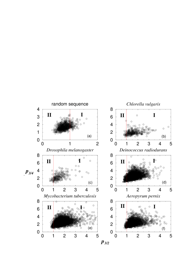
Figure 10: Fluctuations of the probability function ${\mathbf{P}}_{4}(d)$ exhibited through the parameters $p_{3/2}$ and $p_{3/4}$. (a) Plot of $p_{3/2}$ versus $p_{3/4}$ for 4500 random sequences, each one 500 bases in length. (b)-(f) The same as above but using protein-coding sequences of different organisms. The number of points vary in each graph since the available genetic sequences used in the calculations had different lengths. These sequences were divided into small pieces, each one composed of 500 bases. Note that for protein-coding sequences, the majority of the points fall in region I, for which both $p_{3/2}$ and $p_{3/4}$ are greater than 1. Note also the scale on the axes.

$$p_{3/2} = \frac{{\mathbf{P}}_{4}(3)}{{\mathbf{P}}_{4}(2)}$$

$$p_{3/4} = \frac{{\mathbf{P}}_{4}(3)}{{\mathbf{P}}_{4}(4)}$$

If the probability function ${\mathbf{P}}_{4}(d)$ associated with a given sequence has its highest value at $d^{*}=3$, then the corresponding parameters $p_{3/2}$ and $p_{3/4}$ will both be greater than one. Otherwise, one or both of these parameters will be smaller than one.

Fig.10a is a plot of $p_{3/2}$ vs. $p_{3/4}$ for 1000 random sequences, each one consisting of 500 bases (which is a typical length of sequences coding functional proteins [17]). It can be seen from the figure that only a small fraction of the points (about 0.224) fall in region I, for which $p_{3/2}>1$ and $p_{3/4}>1$. The rest of the points fall in region II, in which $p_{3/2}<1$ and $p_{3/4}>1$. Therefore, the probability of having a random sequence, 500 bases long, whose consecutive potential minima are more often separated by a distance $d^{*}=3$, is close to $0.224$.

On the other hand, Figs.10b-f show similar graphs, but using protein-coding sequences of real organisms. These graphs were constructed by analyzing short coding sequences 500 bases in length. The fraction of points falling in region I ($p_{3/2}>1$ and $p_{3/4}>1$) for the different organisms of Fig.10 is summarized in the following table:

Organism	Frac. region I
random sequence	0.224000
Chlorella vulg.	0.788235
Drosophila	0.780220
Deinococcus rad.	0.803525
Myc. tuberculosis	0.802643
Aeropyrum pernix	0.719973

These results show that protein-coding sequences are much more likely to have their consecutive potential minima separated by a distance $d^{*}=3$.

To end this section, we should make a further comment. The fact that the most probable distance $d^{*}$ between consecutive potential minima is $d^{*}=3$ for protein-coding sequences, is a consequence of the order in which the bases or codons appear along the sequence and are not related to the relative weight (fraction) of their occurrence. For example, Fig.11a shows the probability function ${\mathbf{P}}_{4}(d)$ corresponding to a protein-coding sequence of Escherichia coli, 45000 bases in length. In Fig.11b the codon composition, expressed as fractional occurrence, of this sequence is depicted. To construct this last graph, we labelled each codon in an arbitrary way, by assigning an integer number, from 0 for AAA up to 63 for GGG. On the horizontal axis the number of the codon is plotted, and on the vertical axis its fractional occurrence on the E. coli sequence. Finally, Fig.11c shows the probability function ${\mathbf{P}}_{4}(d)$ corresponding to a random sequence, of the same length and codon composition as the one used in Fig.11a. As can be seen, for the “randomized” E. coli sequence the most probable distance is no longer $d^{*}=3$ as in Fig.11a, but $d^{*}=2$.

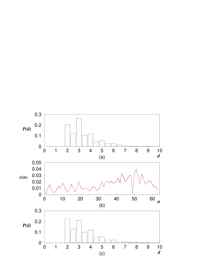
Figure 11: (a) Probability function corresponding to a protein-coding sequence of Escherichia coli. (b) Codon composition $c(n)$ of this E. coli sequence. Each codon was labeled with an integer number $n$, from 0 for AAA up to 63 for GGG. The horizontal axis is the codon number $n$ and the vertical axis is the codon composition $c(n)$ expressed as the fractional occurrence of codon $n$. (c) Probability function corresponding to a random sequence with the same codon composition as in (b). Note that for this randomized sequence, the peak at $d=3$ is lost.

5 Extended chain: $M>1$

In this section we consider the case in which the chain is composed of more than one single monomer. As mentioned before, this reflects the fact that the ribosome is not a point particle after all. At each given time, the ribosome interacts with the mRNA at several points, giving rise to a collective interaction. Electron microscopy has revealed that the mRNA thread passes across the ribosome throughout a tunnel about 10nm long and 2nm in diameter [17]. Since nucleotide length is about 0.5nm, around 20 nucleotides may be in a position to interact simultaneously with the ribosome. Taking the above into account, we will work with a small chain, assuming $M=10$ as a reasonable length.

In the step-like limit, the interaction potential equation can be written by equation (3) now with the variables $\{V_{j}\}$ given by:

$$V_{j}=Kq_{j}\sum_{i=1}^{M}p_{i}$$ (15)

The main modification caused by using equation (15) instead of (7) for the random variables $\{V_{j}\}$ is that they are no longer statistically independent. Due to the collective interaction between the chain and the polymer, these variables are strongly correlated. This makes the problem of finding the probability function ${\mathbf{P}}_{m}(d)$ too difficult for analytical treatment. Therefore, we will present only numerical results.

Figure 12: Two graphs of the probability function ${\mathbf{P}}_{4}(d)$ corresponding to two different realizations of monomer charges for a 10-monomer chain interacting with a 500 monomer polymer. As can be seen, the shape of the probability function depends strongly on the particular realization of charges in the chain. The mean distance $\bar{d}$ is $\bar{d}\simeq 2.36$ for (a) and $\bar{d}\simeq 2.98$ for (b).

In our simulations, ${\mathbf{P}}_{m}(d)$ presents an erratic behavior. The shape of this function strongly depends on the particular realization of monomer charges in the chain. For example, Fig.12a shows the probability function ${\mathbf{P}}_{m}(d)$ for a polymer 500 monomers in length and a particular realization of charges in a 10-monomer chain. The charge values we used to generate these graphs were $\{\pm 1,\pm 2\}$. Fig.12b shows a similar graph but for a different realization of charges along the chain (the realization of charges in the polymer was the same in both cases). As can be seen, these two graphs differ considerably: the first presents a very sharp maximum at $d^{*}=2$, whereas the second does so at $d^{*}=3$. Wide fluctuations in the probability function ${\mathbf{P}}_{m}(d)$ were always present in our numerical simulations.

This fluctuating behavior did not occur in the single-monomer-chain case. It is apparent from Fig.10a that the fluctuations of the probability function ${\mathbf{P}}_{m}(d)$ in that case are rather small: the probability function has its highest value at $d^{*}=2$ for the majority of the realizations (77.6$\%$) in the case $M=1$. Also, the fluctuations are concentrated in a small region of the $(p_{3/2},p_{3/4})$ plane.

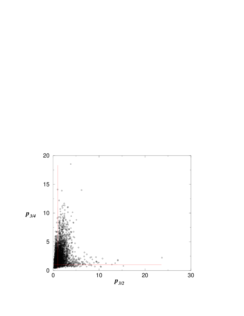
Figure 13: Fluctuations of the probability function exhibited by the parameters $p_{3/2}$ and $p_{3/4}$ for the extended-chain case. A 10-particle chain was used along with a polymer 500 monomers in extent. The graph shows the above parameters for 4500 realizations or monomer charges in the chain. Note that the points spread out over a much wider region than in Fig.10a. Also, in this case the majority of the points fall in the region for which $p_{3/2}>1$ and $p_{3/4}>1$.

In order to have an idea of the magnitude of the fluctuations of the probability function ${\mathbf{P}}_{m}(d)$ in the extended-chain case, we can make use of the parameters $p_{3/2}$ and $p_{3/4}$ defined in expression (LABEL:p32). The fluctuations of the probability function in the extenden-chain case are shown in Fig.13. To construct this figure, a polymer 500 monomers in length was used along with a 10-monomer chain. The charge values in the polymer as well as in the chain were again $\{\pm 1,\pm 2\}$. The parameters $p_{3/2}$ and $p_{3/4}$ were calculated for 4500 charge realizations in the chain (the realization of charges in the polymer was the same in all the cases). Fig.13 is the plot of $p_{3/2}$ versus $p_{3/4}$ for these 4500 realizations. Two remarks are worth mentioning about this figure:

• The points are spread out over a much wider region than in the single-monomer-chain case (Fig.10a).

• The majority of the points fall in the region in which both $p_{3/2}>1$ and $p_{3/4}>1$.

The following table shows the fractions of the points falling in each of the four regions of the graph:

Region	Fraction
$p_{3/2}>1$, $p_{3/4}>1$	0.52978
$p_{3/2}<1$, $p_{3/4}>1$	0.33800
$p_{3/2}>1$, $p_{3/4}<1$	0.07778
$p_{3/2}<1$, $p_{3/4}<1$	0.05444

Therefore, when a collective interaction between the polymer and the chain prevails, a remarkable property arises: The probability of having a random interaction potential, whose consecutive minima are more often separated by three monomers, is the largest.

6 Dynamics

Recent experimental evidence suggests that the ribosome-mRNA system presents a ratchet-like behavior in the protein synthesis translocation process [18]. In this view, the ribosome is tightly attached to the mRNA thread in the absence of GTP. This is so because the channel in the ribosome through which the mRNA passes, is more or less closed. When a GTP molecule is supplied (and transformed into GDP), this channel opens leaving the mRNA thread free to move one codon. Subsequently the mRNA passage in the ribosome closes again, trapping the mRNA molecule.

In this clamping mechanism several physicochemical factors are involved, which if taken into account in detail would lead to complex dynamical equations hard to handle. In this work our approach is to look into the behavior of oversimplified molecular models which might capture some of the essential dynamical features of the system and may shed some light on how this mechanism could have arisen in the origin of life conditions.

In our modelling the dynamics of the system is governed by the application of an external force $F_{ex}$ to the chain in the horizontal direction, i.e. parallel to the polymer. By this means the chain will be forced to move along the polymer. In principle, the force $F_{ex}$ may be time dependent, but we will restrict ourselves to a constant term. This force might come from a chemical pump (like GDP) or from any other electromagnetic force present in prebiotic conditions. The only purpose of this force in our model is to drive the chain along the polymer (which is assumed to be fixed, $N\rightarrow\infty$ limit), avoiding it from getting trapped in some of the minima of the polymer-chain interaction potential $V(x)$. Therefore, we will also assume that $F_{ex}$ satisfies $|F_{ex}|>$ max$|\partial V(x)/\partial x|$.

Our analysis relies on Newton’s equation of motion in a high friction regime, where inertial effects can be neglected. This regime actually exists in biological molecular ratchets similar to the one we are considering [19, 20]. Under such conditions, the Newton’s equation of motion acquires the form

$$\gamma\frac{dx}{dt}=-\frac{\partial V_{\sigma}^{\alpha}(x)}{\partial x}+F_{ex}$$ (16)

where $\gamma$ is the friction coefficient. In what follows, we will set $\gamma=1$, which is equivalent to setting the measure of the time unit. The above, though a deterministic equation, gives rise to a random dynamics due to the randomness of the interaction potential $V_{\sigma}^{\alpha}(x)$. In order to start analyzing this random dynamics, let us consider first the single-monomer-chain case $M=1$. In this case, as before, we will refer to the chain simply as “the particle”.

6.1 Single-monomer chain: $M=1$. Random sequences.

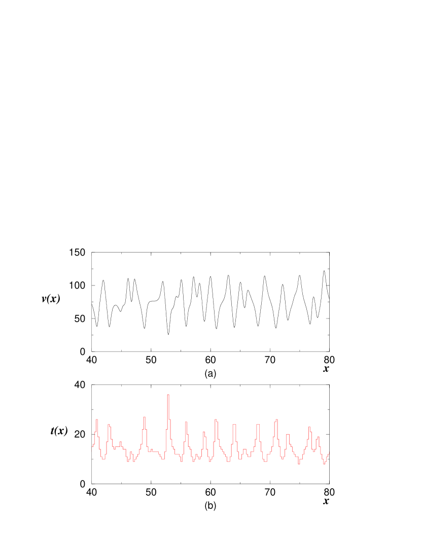
Figure 14: (a) Typical realization of the velocity of the particle along the polymer as a function of the position $x$. (b) Local transit time $t$ as a function of the position $x$. Note that the particle effectively spends more time in certain regions of the polymer than in others. Also, note the regularity in the positions of the maxima of the local transit time.

In Fig.14a we show a typical realization of the velocity of the particle $v(x)$ as a function of its position $x$ along the polymer. This graph was constructed by solving numerically the equation of motion (16), using the fourth order Runge-Kuta method. The parameter values used were $\alpha=2$ and $\sigma=0.5$, and the monomer charge values were $\{\pm 1,\pm 2\}$ (case $m=4$). Fig.14b shows the local-transit times of the particle along a short segment of the polymer (40 monomers in length). This transit time is represented in arbitrary units, and was computed by counting how many time steps the particle spent in every spatial interval $\Delta x$ throughout the polymer. In the graph shown, the value of $\Delta x$ was $\Delta x=0.25$. It is apparent from this figure that, in its way along the polymer, the particle spends more time in certain regions than in others, the former being more or less regularly spaced along the polymer.

In order to find out the spatial regularities in the dynamics of the system, it is convenient to take the Fourier transform of the velocity $v(x)$ of the particle. Let us call $\hat{v}(k)$ the Fourier transform of $v(x)$, $k$ being the Fourier variable conjugate to $x$.

Figure 15: Power spectrum of the velocity of the particle along the polymer, for two random realizations of monomer charges in the polymer. Note that there exist dominant frequencies $k^{*}$ even though the charges of the polymer were assigned at random. These dominant frequencies correspond to spatial regularities $\lambda^{*}=2\pi/k^{*}$ with values (a) $\lambda^{*}\simeq 3.29$ and (b) $\lambda^{*}\simeq 3.30$.

Fig.15 shows the Fourier power spectrum of the velocity, $|\hat{v}(k)|^{2}$, for two different realizations of monomer charges in the polymer. The parameter values in Fig.15a and Fig.15b are $\{\sigma=0.5,\ \alpha=1\}$ and $\{\sigma=0.5,\ \alpha=4\}$ respectively. These graphs were computed for the case $m=4$, using the charge values $\{\pm 1,\pm 2\}$. From the figure, it is evident that there exists a dominant frequency $k^{*}$ in the power spectrum of the velocity (the highest peak), whose corresponding spatial periodicity is $\lambda^{*}=2\pi/k^{*}\sim 3.3$. The power spectrum reveals a dynamical regularity in the motion of the particle throughout the polymer. This regularity is inherited from the one present in the random potential, in the sense that the particle spends more time in the minima than in the maxima. The consequence is a slowing down of the velocity nearly every three monomers, which is reflected in the power spectrum. Our interpretation is that the peak occurring in the power spectrum of the velocity conveys the information on the average distance $\bar{d}$ between consecutive potential minima, which for the case $m=4$ is $\bar{d}\sim 3.4$.

6.2 Single-monomer chain: $M=1$. Real sequences.

As in section 4, we can assign the charges along the polymer in correspondence with the genetic sequence of real organisms. In order to do that, we will use the same base-charge correspondence as in expression (13). The objective is to find out how the dynamics of the system changes when using real genetic sequences instead of random ones. In what follows, the value of the parameters $\alpha$ and $\sigma$ will be $\alpha=1$, $\sigma=0.5$.

Figure 16: Power spectrum of the velocity of the particle using protein-coding sequences of different organisms to assign the charges on the polymer. Note the very sharp peaks in all the spectra. The above means that the dynamics generated by protein-coding sequences presents very well defined periodicities. Also, note that these spatial periodicities are almost equal to 3. The peak around $k=4$ is a resonant frequency (second harmonic) of the first peak.

Figure 17: Power spectrum of the velocity of the particle using non-coding sequences of S. cerevisiade (yeast) and C. elegans (worm). In this case the spatial periodicity is weaker (or absent) than in Fig.16. It seems that the non-coding sequences of real organisms have a random like structure.

The power spectrum of the velocity of the particle throughout the polymer, when using protein-coding sequences of different organisms, is shown in Fig.16. To generate these graphs, short coding sequences of several organisms, each 10000 monomers in length, were used. Two points are worth noticing in this figure. First, the peak in the power spectrum is much higher than in the random case. This indicates that there is a much more well defined periodicity in the dynamics generated by interaction potentials when protein-coding sequences are used. Second, the spatial periodicity reflected in the peak of the power spectrum is much closer to $3$ than in the random case.

This dynamical behavior is not present when real but non-coding sequences are used. For example, in Fig.17 we show the power spectrum of the velocity of the particle along the polymer, for two cases in which the monomer charges in the polymer were assigned in correspondence with intergenic regions of two organisms. As can be seen, the structure of such spectra is similar to the one obtained in the random case. In this sense, intergenic regions again seem to have a random structure.

The fact that the power spectrum corresponding to protein-coding sequences exhibits a very sharp periodicity at $\lambda^{*}\simeq 3$, whereas the one corresponding to non-coding sequences does not, has already been reported in the literature [21]. Nonetheless, in these previous works the power spectrum of the “bare” genetic sequences is analyzed, namely, without considering any kind of interaction potential or dynamical behavior. What we have shown here, though, is that this “structural” periodicity around three transforms into a dynamical periodicity in the motion of the particle along the polymer.

6.3 Extended chain: M=10

The most interesting dynamics occurs when an extended chain is interacting with the polymer. In such a situation, a collective interaction prevails. At every moment there are several contact points between the chain and the polymer. As we have already pointed out, collective interaction between the chain and the polymer gives rise to a widely fluctuating probability function ${\mathbf{P}}_{m}(d)$. The same occurs with the power spectrum of the velocity of the chain along the polymer. However, these fluctuations, far from being annoying, produce a much richer dynamical behavior than in the single-monomer-chain case.

In Fig.18 we show the power spectra of the velocity of the chain along the polymer for two different random realizations of monomer charges in the chain. The charges in the polymer were the same in both cases. These graphs were constructed with a polymer 500 monomers in length and a 10-monomer chain. The parameter values used were $\sigma=0.5$ and $\alpha=1$. Also, the charge values were, as above $\{\pm 1,\ \pm 2\}$. From the figure, it is apparent that the power spectrum of the velocity exhibits a very well defined dominant frequency, even though the charges in both the polymer and the chain were assigned at random. The power spectrum in Fig.18a presents a dominant frequency corresponding to a spatial periodicity $\lambda^{*}\simeq 2$, whereas the corresponding periodicity in the power spectrum shown in Fig.18b is $\lambda^{*}\simeq 3$. We should explain this difference.

Figure 18: Power spectrum of the velocity of a 10-monomer chain along a polymer 500 monomers in length. These two graphs correspond to two different random realizations of monomer charges in the chain. (a) The spatial periodicity is $\lambda^{*}\simeq 2.01$ and (b) $\lambda^{*}\simeq 2.88$. In (a) the corresponding probability function had a shape like the one in Fig.12a with $d^{*}=2$ and $bar{d}\simeq 2$, whereas in (b) the probability function was as in Fig.12b with $d^{*}=3$ and $\bar{d}\simeq 3$. In the extended-chain case, there is a finite correlation lengt along the potential (equal to the size of the chain), which is reflected in the little “heaps” appearing in the power spectrum.

The power spectrum appearing in Fig.18a was constructed by using a polymer and a chain whose associated probability function ${\mathbf{P}}_{4}(d)$ has the same shape as the one of Fig.12a. Namely, for this system the probability function has a very high value at $d^{*}=2$. On the other hand, the power spectrum in Fig.18b corresponds to a system whose probability function has a very sharp peak at $d^{*}=3$, as the one shown in Fig.12b. From our numerical simulations, we can conclude that whenever the probability function has a sharp maximum at a distance $d^{*}$, the power spectrum of the velocity also presents a sharp peak corresponding to a spatial periodicity $\lambda^{*}=d^{*}$.

As we have seen, in the collective-interaction case the most probable configurations are those in which the probability function ${\mathbf{P}}_{4}(d)$ has its highest value at $d^{*}=3$ (see Fig.13). Therefore, if we assign at random the monomer charges in the polymer and in the chain, with high probability we will come up with a dynamics possessing a very well defined periodicity: the chain will move along the polymer in “jumps” whose length is nearly three monomers.

7 Summary and discussion

The results presented throughout this work suggest a possible scenario for the origin of the three base codon structure of the genetic code. In this scenario, primitive one dimensional molecular machines, initially with a random structure, exhibited a regular dynamics with a “preference” for a movement in steps of three bases. By “steps” we mean a slowing down of the velocity of the chain along the polymer, nearly every three monomers (see Fig.14b). Even in the simplest case in which the chain consists of only one monomer, the above dynamical regularity is apparent. We can think of the dynamics of primitive molecular machines as being “biased towards three”.

The preceding property is quite robust inasmuch as it hardly depends on the particular kind of interaction between the polymer and the chain. On one hand, the kind of electrostatic potentials we have used is representative of the actual interaction potentials between particles occurring in Nature. These potentials are characterized in our model by the parameter $\alpha$. We have also seen that the distribution distances between neighboring maxima and minima along the interaction potential, characterized by the probability function ${\mathbf{P}}_{m}(d)$, does not depend on this parameter (for small values of $\sigma$), i.e. it will be the same whether the interaction is coulombian or dipolar or of any other (electrostatic) type.

On the other hand, the spatial distribution of interaction potential minima also does not depend on the particular values of the monomer charges $\{q_{j}\}$ and $\{p_{i}\}$, as long as these values are of the same order of magnitude. An important feature that the charges must comply with is that they take more than two different values. This allows for an order relation to be established among the different types of monomers, leading to a maxima and minima structure of the interaction potential. The probability function ${\mathbf{P}}_{m}(d)$, which gives the probability of two consecutive minima being separated by a distance $d$, only depends on $m$, namely, on the number of different types of monomers. As $m$ increases, the mean distance $\bar{d}$ between consecutive potential minima approaches three. Nevertheless, in the particle (single-monomer-chain) case, the most probable distance is $d^{*}=2$ (for $m>2$).

Still in this particle case, considerable changes take place when the charges along the polymer are assigned in correspondence with protein-coding genetic sequences of real organisms. In this case, not only is the mean distance $\bar{d}$ between neighboring potential minima nearly three, but also the most probable one, $d^{*}$, happens to be three. This is a remarkable property of protein-coding sequences, perhaps acquired throughout evolution. Furhtermore the fact that this “refinement” is absent in non-coding sequences of real organisms, strongly suggests that it is a consequence of the dynamical processes involved in the protein synthesis mechanisms.

This interpretation is supported by the results obtained when the dynamics of the particle moving along the polymer is considered. In the random sequence case, there are dominant frequencies in the power spectrum of the particle velocity related with the spatial regularities of the interaction potential. Moreover in the protein-coding sequence case, the power spectrum of the velocity shows a very well defined periodicity corresponding almost exactly to a spatial distance $\lambda^{*}=3$. Again, this behavior does not occur for non-coding sequences of real organisms, which are not involved in the translation processes.

A richer dynamics emerges when the chain is composed of several monomers. In this, more realistic, collective-interaction case, the probability function ${\mathbf{P}}_{m}(d)$ presents very wide fluctuations, depending on the particular assignment of monomer charges in the chain. Nevertheless, the most probable configurations are those for which the probability function has its highest value at $d^{*}=3$. For these configurations, the power spectrum of the chain velocity along the polymer exhibits a very well defined spatial periodicity at $\lambda^{*}\simeq 3$.

Our results suggest an origin of life scenario in which primordial molecular machines of chains moving along polymers in quasi one-dimensional geometries, that eventually led to the protein synthesis processes, were biased towards a dynamics favoring the motion in “steps” or “jumps” of three monomers. The higher likelyhood of these primitive“ribosomes” may have led to the present ribosomal dynamics where mRNA moves along rRNA in a channel conformed by the ribosome. Dynamics may have acted in this sense as one of the evolutionary filter favoring the three base codon composition of the genetic code.

Acknowledgements
We would like to thank Leo Kadanoff, Sue Coppersmith, Haim Diamant and Cristian Huepe for very useful discussions and corrections. This work was sponsored by the DGAPA-UNAM project IN103300, the MRSEC Program of the National Science Foundation (NSF) under Award Number DMR 9808595 and by the NSF Program DMR 0094569. M. Aldana also acknowledges CONACyT-México a posdoctoral grant.

References

- [1] Martínez-Mekler G, Aldana M, Cázarez-Bush F, Garcia-Pelayo R, Cocho G (1999) Primitive molecular machine scenario for the origin of the three base codon composition. Org Life Evol Bios 29:203-214
- [2] Aldana M, Cázarez-Bush F, Cocho G, Martínez-Mekler G (1998) Primordial synthesis machines and the origin of the genetic code. Physica A 257:119-127
- [3] Martínez-Mekler G, Aldana M, Cocho G (1999) On the role of molecular machines in the origin of the genetic code, in ”Statistical mechanics of biocomplexity: proceedings of the XV Sitges Conference, held at Sitges, Barcelona, Spain 8-12 June 1998”, editors Reguera D, Vilar JMG, Rubi JM, (Springer Verlag Lecture Notes in Physics 527:112-123).
- [4] Alberti S (1997) The origin of the genetic code and protein Synthesis. J Mol Evol 45:352-358
- [5] Alberti S (1999) Evolution of the genetic code, protein synthesis and nucleic acid replication. Cell Mol Life Sci 56:85-93
- [6] Amirnovin R (1997) An analysis of the metabolic theory of the origin of the genetic code. J Mol Evol 44:473-476
- [7] Di Gulio M, Medugno M (1998) The historical factor: the biosynthetic relationships between amino acids and their physicochemical properties in the origin of the genetic code. J Mol Evol 46:615-621
- [8] Di Gulio M (1997) On the origin of the genetic code. J Theor Biol 191:573-581
- [9] Freeland SJ, Laurence DH (1998) The genetic code is one in a million. J Mol Evol 47:238-248
- [10] Brener S, Jacob F, Meselson M (1961) An unstable intermidiate carrying information from genes to ribosomes for protein synthesis. Nature 190:575-80
- [11] Brenner S (1989) Molecular Biology: A selection of papers (Academic Press, Orlando, Fl).
- [12] Lehninger AL, Nelson DL, Cox MM (2000) Principles of biochemestry. W H Freeman and Co. Third edition.
- [13] Doig AJ (1997) Inproving the efficency of the genetic code by varying the codon length: the perfect genetic code. J. Theor Biol 188:355-360
- [14] Gilbert W (1986) The RNA world. Nature 319:618-625
- [15] Aldana M, Cocho G, Larralde H, Martínez-Mekler G, CCF-UNAM preprint to be submitted for publication.
- [16] MacKerell Jr AD, Wiórkiewicz-Kuczera J, Karplus M (1995) An all-atom empirical energy function for the simulation of nucleic acids. J Am Chem Soc 117:11946-11975
- [17] Lewin B (1999) Genes VII. Oxford University Press.
- [18] Frank J, Agrawal RK (2000) A ratchet-like inter-subunit reorganization of the ribosome during translocation. Nature 405:318-322
- [19] Bier M (1997) Brownian ratchets in physics and biology. Cont Phys 38(6):371-379
- [20] Jülicher F, Ajdari A, Prost J (1997) Modeling molecular motors. Rev Mod Phys 69(4):1269-1281
- [21] Lobzin VV, Chechetkin VR (2000) Order and correlations in DNA sequences. The spectral approach. Physics-Uspekhi 43(1):55-78