Mark correlations: relating physical properties to spatial distributions

Abstract

Mark correlations provide a systematic approach to look at objects both distributed in space and bearing intrinsic information, for instance on physical properties. The interplay of the objects’ properties (marks) with the spatial clustering is of vivid interest for many applications; are, e.g., galaxies with high luminosities more strongly clustered than dim ones? Do neighbored pores in a sandstone have similar sizes? How does the shape of impact craters on a planet depend on the geological surface properties? In this article, we give an introduction into the appropriate mathematical framework to deal with such questions, i.e. the theory of marked point processes. After having clarified the notion of segregation effects, we define universal test quantities applicable to realizations of a marked point processes. We show their power using concrete data sets in analyzing the luminosity-dependence of the galaxy clustering, the alignment of dark matter halos in gravitational $N$-body simulations, the morphology- and diameter-dependence of the Martian crater distribution and the size correlations of pores in sandstone. In order to understand our data in more detail, we discuss the Boolean depletion model, the random field model and the Cox random field model. The first model describes depletion effects in the distribution of Martian craters and pores in sandstone, whereas the last one accounts at least qualitatively for the observed luminosity-dependence of the galaxy clustering.

draft

0.1 Marked point sets

Observations of spatial patterns at various length scales frequently are the only point where the physical world meets theoretical models. In many cases these patterns consist of a number of comparable objects distributed in space such as pores in a sandstone, or craters on the surface of a planet. Another example is given in Figure 1, where we display the galaxy distribution as traced by a recent galaxy catalogue. The galaxies are represented as circles centered at their positions, whereas the size of the circles mirrors the luminosity of a galaxy. In order to test to which extent theoretical predictions fit the empirically found structures of that type, one has to rely on quantitative measures describing the physical information. Since theoretical models mostly do not try to explain the structures individually, but rather predict some of their generic properties, one has to adopt a statistical point of view and to interpret the data as a realization of a random process. In a first step one often confines oneself to the spatial distribution of the objects constituting the patterns and investigates their clustering thereby thinking of it as a realization of a point process. Assuming that perspective, however, one neglects a possible linkage between the spatial clustering and the intrinsic properties of the objects. For instance, there are strong indications that the clustering of galaxies depends on their luminosity as well as on their morphological type. Considering Figure 1, one might infer that luminous galaxies are more strongly correlated than dim ones. Effects like that are referred to as mark segregation and provide insight into the generation and interactions of, e.g., galaxies or other objects under consideration. The appropriate statistical framework to describe the relation between the spatial distribution of

Figure 1: The galaxy distribution as traced by the Southern Sky Redshift Survey 2 (SSRS 2). We show a part of the sample investigated, projected down into two dimensions. Each circle represents a galaxy, its radius is proportional to the galaxy’s luminosity. For further details see Section 0.2.1.

physical objects and their inner properties are marked point processes, where discrete, scalar-, or vector-valued marks are attached to the random points.
In this contribution we outline how to describe marked point processes; along that line we discuss two notions of independence (Section 0.1) and define corresponding statistics that allow us to quantify possible dependencies. After having shown that some empirical data sets show significant signals of mark segregation (Section0.2), we turn to analytical models, both motivated by mathematical and physical considerations (Section 0.3).
Contact distribution functions as presented in the contribution by D. Hug et al. in this volume are an alternative technique to measure and statistically quantify distances which finally can be used to relate physical properties to spatial structures. Mark correlation functions are useful to quantify molecular orientations in liquid crystals (see the contribution by F. Schmid and N. H. Phuong in this volume) or in self-assembling amphiphilic systems (see the contribution by U. S. Schwarz and G. Gompper in this volume). But also to study anisotropies in composite or porous materials, which are essential for elastic and transport properties (see the contributions by D. Jeulin, C. Arns et al. and H.-J. Vogel in this volume), mark correlations may be relevant.

0.1.1 The framework

The empirical data – the positions ${\mathbf{x}}_{i}$ of some objects together with their intrinsic properties $m_{i}$ – are interpreted as a realization of a marked point process $\{({\mathbf{x}}_{i},m_{i})\}_{i=1}^{N}$ (Stoyan, Kendall and Mecke, 1995). For simplicity we restrict ourselves to homogeneous and isotropic processes.
The hierarchy of joint probability densities provides a suitable tool to describe the stochastic properties of a marked point process. Thus, let $\varrho_{1}^{{\cal S}{\cal M}}\left(({\mathbf{x}},m)\right)$ denote the probability density of finding a point at ${\mathbf{x}}$ with a mark $m$. For a homogeneous process this splits into $\varrho_{1}^{{\cal S}{\cal M}}\left(({\mathbf{x}},m)\right)=\varrho{\cal M}_{1}(m)$ where $\varrho$ denotes the mean number density of points in space and ${\cal M}_{1}(m)$ is the probability density of finding the mark $m$ on an arbitrary point. Later on we need moments of this mark distribution; for real-valued marks the $k$th-moment of the mark-distribution is defined as

$$\overline{m^{k}}=\int{\rm d}m\ {\cal M}_{1}(m)m^{k};$$ (1)

the mark variance is $\sigma_{M}^{2}=\overline{m^{2}}-\overline{m}^{2}$.
Accordingly, $\varrho_{2}^{{\cal S}{\cal M}}\left(({\mathbf{x}}_{1},m_{1}),({\mathbf{x}}_{2},m_{2})\right)$ quantifies the probability density to find two points at ${\mathbf{x}}_{1}$ and ${\mathbf{x}}_{2}$ with marks $m_{1}$ and $m_{2}$, respectively (for second-order theory of marked point processes see kerscher_stoyan:stochgeom ; kerscher_stoyan:fractals ). It effectively depends only on $m_{1}$, $m_{2}$, and the pair separation $r=|{\mathbf{x}}_{2}-{\mathbf{x}}_{1}|$ for a homogeneous and isotropic process. Two-point properties certainly are the simplest non-trivial quantities for homogeneous random processes, but it may be necessary to move on to higher correlations in order to discriminate between certain models.

0.1.2 Two notions of independence

In the following we will discuss two notions of independence, which may arise for marked point patterns. For this, consider two Renaissance families, call them the Sforza and the Gonzaga. They used to build castles spread out more or less homogeneously over Italy. In order to describe this example in terms of a marked point process, we consider the locations of the castles as points on a map of Italy, and treat a castle’s owner as a discrete mark, $S$ and $G$, respectively. There are many ways how the castles can be built and related to each other.

Independent sub-point processes:

For example, the Sforza may build their castles regardless of the Gonzaga castles. In that case the probability of finding a Sforza castle at ${\mathbf{x}}_{1}$ and a Gonzaga castle at ${\mathbf{x}}_{2}$ factorizes into two one-point probabilities and we can think of the Sforza and the Gonzaga castles as uncorrelated sub-point processes. In the language of marked point processes this means, e.g., that

$$\begin{split}\varrho_{2}^{{\cal S},{\cal M}}\left(({\mathbf{x}}_{1},m_{1}),({\mathbf{x}}_{2},m_{2})\right)&=\varrho_{1}^{{\cal S}{\cal M}}\left(({\mathbf{x}}_{1},m_{1})\right)\varrho_{1}^{{\cal S}{\cal M}}\left(({\mathbf{x}}_{2},m_{2})\right)\\ &=\varrho^{2}{\cal M}_{1}(m_{1}){\cal M}_{1}(m_{2}),\end{split}$$ (2)

for any $m_{1}\neq m_{2}$. If all the joint $n$-point densities factorize into a product of $n^{\prime}$-point densities of one type each, then we speak of independent sub-point processes. Dependent sub-point processes indicate interactions between points of different marks; for instance, the Gonzaga may build their castles close to the Sforza ones in order to avoid that a region becomes dominated by the other family’s castles.

Mark-independent clustering:

A second type of independence refers to the question whether the different families have different styles to plan their castles. For instance, the Gonzaga may distribute their castles in a grid-like manner over Italy, whereas the Sforza may incline to build a second castle close to each castle they own. Rather than asking whether two sub-point processes (namely the Gonzaga and the Sforza castles, respectively) are independent (“independent sub-point processes”), we are now discussing whether they are different as regards their statistical clustering properties. Any such difference means that the clustering depends on the intrinsic mark of a point.
Whenever the two-point probability density of finding two objects at ${\mathbf{x}}_{1}$ and ${\mathbf{x}}_{2}$ depends on the objects’ intrinsic properties we speak of mark-dependent clustering. It is useful to rephrase this statement by using Bayes’ theorem and the conditional mark probability density

$${\cal M}_{2}(m_{1},m_{2}|{\mathbf{x}}_{1},{\mathbf{x}}_{2})=\frac{\varrho_{2}^{{\cal S},{\cal M}}\left(({\mathbf{x}}_{1},m_{1}),({\mathbf{x}}_{2},m_{2})\right)}{\varrho_{2}^{{\cal S}}\left({\mathbf{x}}_{1},{\mathbf{x}}_{2}\right)},$$ (3)

in case the spatial product density $\varrho_{2}^{{\cal S}}(\cdot)$ does not vanish. ${\cal M}_{2}(m_{1},m_{2}|{\mathbf{x}}_{1},{\mathbf{x}}_{2})$ is the probability density of finding the marks $m_{1}$ and $m_{2}$ on objects located at ${\mathbf{x}}_{1}$ and ${\mathbf{x}}_{2}$, given that there are objects at these points. Clearly, ${\cal M}_{2}(m_{1},m_{2}|{\mathbf{x}}_{1},{\mathbf{x}}_{2})$ depends only on the pair separation $r=|{\mathbf{x}}_{1}-{\mathbf{x}}_{2}|$ for homogeneous and isotropic point processes. We speak of mark-independent clustering, if ${\cal M}_{2}(m_{1},m_{2}|r)$ factorizes

$${\cal M}_{2}(m_{1},m_{2}|r)={\cal M}_{1}(m_{1}){\cal M}_{1}(m_{2})$$ (4)

and thus does not depend on the pair separation. That means that regarding their marks, pairs with a separation $r$ are not different from any other pairs. On the contrary, mark-dependent clustering or mark segregation implies that the marks on certain pairs show deviations from the global mark distribution.
In order to distinguish between both sorts of independencies, let us consider the case where we are given a map of Italy only showing the Gonzaga castles. If the distribution of castles in Italy can be understood as consisting of independent sub-point processes, we cannot infer anything about the Sforza castles from the Gonzaga ones. However, if $\varrho_{2}^{{\cal S},{\cal M}}\left(({\mathbf{x}}_{1},S),({\mathbf{x}}_{2},G)\right)>\varrho^{2}{\cal M}_{1}(S){\cal M}_{1}(G)$, Sforza castles are likely to be found close to Gonzaga ones. Here, ${\cal M}_{1}(S)$ and ${\cal M}_{1}(G)$ are the probabilities that a castle belongs to the Sforza or Gonzaga family. If, on the other hand, mark-independent clustering applies, typical clustering properties such as the spatial clustering strength are equal for both castle distributions, and the Gonzaga castles are in the statistical sense already representative of the whole castle distribution in Italy. That means in particular that, if the Gonzaga castles are clustered, so are the Sforza ones.

Before we turn to applications, we have to develop practical test quantities in order to test for segregation effects in real data and to describe them in more detail.

0.1.3 Investigating the independence of sub-point processes

To investigate correlations between sub-point processes, suitably extended nearest neighbor distribution functions or $K$-functions have been employed kerscher_cox:point ; kerscher_diggle:statistical . Also the (conditional) cross-correlation functions can be used (see Eq. 8), for a further test see kerscher_stoyan:fractals , p. 302. Here we consider a multivariate extension of the $J$-function kerscher_vanlieshout:j , as suggested by kerscher_vanlieshout:indices .
For this, consider the nearest neighbor’s distance distribution from an object with mark $m_{i}$ to other objects with mark $m_{j}$, $G_{ij}(r)$ (“$i$ to $j$”, for details see kerscher_vanlieshout:indices ). Let $G_{i\circ}(r)$ denote the distribution of the nearest neighbor’s distance from an object of type $i$ to any other object (denoted by $\circ$). Finally, $G_{\circ\circ}(r)$ is the nearest neighbor distribution of all points. Similar extensions of the empty space function are possible, too. Let $F_{i}(r)$ denote the distribution of the nearest $i$-object’s distance from an arbitrary position, whereas $F_{\circ}(r)$ is the nearest object’s distance distribution from a random point in space to any object in the sample. We consider the following quantities:

$$\begin{split}J_{ij}(r)=\frac{1-G_{ij}(r)}{1-F_{j}(r)},\ J_{i\circ}(r)=\frac{1-G_{i\circ}(r)}{1-F_{\circ}(r)},\ J(r)=\frac{1-G_{\circ\circ}(r)}{1-F_{\circ}(r)},\end{split}$$ (5)

They are defined whenever $F_{j}(r),F_{\circ}(r)<1$. If two sub-point processes, defined by marks $i\neq j$, are independent then one gets kerscher_vanlieshout:indices

$$J_{ij}(r)=1.$$ (6)

Note, that the $J_{ij}$ depend on higher-order correlations functions, similar to the $J$-function kerscher_kerscher:constructing . Suitable estimators for these $J$-functions are derived from estimators of the $F$ and $G$-functions kerscher_stoyan:stochgeom ; kerscher_baddeley:sampling .

0.1.4 Investigating mark segregation

In order to quantify the mark-dependent clustering or to look for the mark segregation, it proves useful to integrate the conditional probability density ${\cal M}_{2}(m_{1},m_{2}|r)$ over the marks weighting with a test function $f(m_{1},m_{2})$ kerscher_stoyan:oncorrelations ; kerscher_stoyan:stochgeom . This procedure reduces the number of variables and leaves us with the weighted pair average:

$$\left\langle f\right\rangle_{\rm P}=\int{\rm d}{m_{1}}\int{\rm d}{m_{2}}\ f(m_{1},m_{2}){\cal M}_{2}(m_{1},m_{2}|r).$$ (7)

The choice of an appropriate weight-function depends on whether the marks are non-quantitative labels or continuous physical quantities.

1. For labels only combinations of indicator-functions are possible, the integral degenerates into a sum over the labels. Supposed the marks of our objects belong to classes labelled with $i,j,\ldots$, the conditional cross-correlation functions are given by

   $$C_{ij}(r)\equiv\left\langle\delta_{m_{1}i}\delta_{m_{2}j}+(1-\delta_{ij})\delta_{m_{2}i}\delta_{m_{1}j}\right\rangle_{\rm P}(r),$$ (8)

   with the Kronecker $\delta_{m_{1}i}=1$ for $m_{1}=i$ and zero otherwise. Mark segregation is indicated by $C_{ij}\neq 2\varrho_{i}\varrho_{j}/\varrho^{2}$ for $i\neq j$ and $C_{ii}\neq\varrho_{i}^{2}/\varrho^{2}$, where $\varrho_{i}$ denotes the number density of points with label $i$. The $C_{ij}$ are cross-correlation functions under the condition that two points are separated by a distance of $r$ (compare kerscher_stoyan:fractals , p. 264, for applications see the Martian crater distribution studied in Sect. 0.2.3 and Figure 7 in particular).

2. For positive real-valued marks $m$, the following pair averages prove to be powerful and distinctive kerscher_schlather:mark ; kerscher_beisbart:luminosity :
   

   1. One of the most simplest weights to be used is the mean mark:

      $$k_{m}(r)\equiv\frac{\left\langle m_{1}+m_{2}\right\rangle_{\rm P}(r)}{2\ \overline{m}}.$$ (9)

      quantifies the deviation of the mean mark on pairs with separation $r$ from the overall mean mark $\overline{m}$. A $k_{m}>1$ indicates mark segregation for point pairs with a separation $r$, specifically their mean mark is then larger than the overall mark average.
      Closely related is Stoyan’s $k_{mm}$ function using the squared geometric mean of the marks as a weight kerscher_stoyan:oncorrelations ; kerscher_stoyan:fractals

      $$k_{mm}(r)\equiv\frac{\left\langle m_{1}m_{2}\right\rangle_{\rm P}(r)}{\overline{m}^{2}}.$$ (10)

   2. Accordingly, higher moments of the marks may be used to quantify mark segregation, like the mark fluctuations

      $${{\text{{\it var}}}}(r)\equiv\left\langle\left(m_{1}-\left\langle m_{1}\right\rangle_{\rm P}(r)\right)^{2}\right\rangle_{\rm P}(r),$$ (11)

      or the mark-variogram kerscher_waelder:variograms ; kerscher_stoyan:variograms :

      $$\gamma(r)\equiv\left\langle\tfrac{1}{2}\left(m_{1}-m_{2}\right)^{2}\right\rangle_{\rm P}(r),$$ (12)

   3. The mark covariance kerscher_cressie:statistics is

      $${{\text{{\it cov}}}}(r)\equiv\left\langle m_{1}m_{2}\right\rangle_{\rm P}(r)-\left\langle m_{1}\right\rangle_{\rm P}(r)\left\langle m_{2}\right\rangle_{\rm P}(r).$$ (13)

      Mark segregation can be detected by looking whether ${{\text{{\it cov}}}}(r)$ differs from zero. A ${{\text{{\it cov}}}}(r)$ larger than zero, e.g., indicates that points with separation $r$ tend to have similar marks. Sometimes the mark covariance is normalized by the fluctuations kerscher_isham:marked : ${{\text{{\it cov}}}}(r)/{{\text{{\it var}}}}(r)$.

   These conditional mark correlation functions can be calculated from only three independent pair averages kerscher_schlather:mark : $\left\langle m\right\rangle_{\rm P}(r)$, $\left\langle m_{1}m_{2}\right\rangle_{\rm P}(r)$, and $\left\langle m^{2}\right\rangle_{\rm P}(r)$. Thus the above mentioned characteristics are not independent, e.g. ${{\text{{\it var}}}}(r)=\gamma(r)+cov(r)$.
   We apply these mark correlation functions to the galaxy distribution in Section 0.2.1 (Figure 3), to Martian craters in Section 0.2.3 (Figure 7) and to pores in sandstones considered in Section 0.2.4.

3. Also vector-valued information ${\mathbf{l}}_{i}$, describing, e.g., the orientation of an anisotropic object at position ${\mathbf{x}}_{i}$ may be available. It is therefore interesting to consider vector marks such as done by kerscher_ohser:onsecond ; kerscher_penttinen:statistical ; kerscher_stoyan:fractals who use a mark correlation function to quantify the alignment of vector marks. Here we suggest three mark correlation functions quantifying geometrically different possibilities of an alignment. In order to ensure coordinate-independence of our descriptors, we focus on scalar combinations of the vector marks in using the scalar product $\cdot$ and the cross product $\times$. Different from the case of scalar marks, it is a non-trivial task to find a set of vector-mark correlation functions which contain all possible information (at least up to a fixed order in mark space). We provide a systematic account of how to construct suitable vector-mark correlation functions in a complete and unique way for general dimensions in the Appendix.
   Here we only cite the most important results. For that we need the distance vector between two points, ${\mathbf{r}}\equiv{\mathbf{x}}_{1}-{\mathbf{x}}_{2}$, the normalized distance vector, $\hat{\mathbf{r}}\equiv{\mathbf{r}}/r$, and the normalized vector mark: $\hat{\mathbf{l}}_{i}\equiv{\mathbf{l}}_{i}/l_{i}$ with $l_{i}=|{\mathbf{l}}_{i}|$. The following conditional mark correlation functions will be used to quantify alignment effects:

   1. ${\cal A}(r)$ quantifies the ${\cal A}$lignment of the two vector marks ${\mathbf{l}}_{1}$ and ${\mathbf{l}}_{2}$:

      $${\cal A}(r)=\frac{1}{\overline{l}^{2}}\left\langle{\mathbf{l}}_{1}\cdot{\mathbf{l}}_{2}\right\rangle_{\rm P}(r)\;\;\;.$$ (14)

      It is proportional to the cosine of the angle between ${\mathbf{l}}_{1}$ and ${\mathbf{l}}_{2}$. We normalize with the mean $\overline{l}$. For purely independent vector marks ${\cal A}(r)$ is zero, whereas ${\cal A}(r)>0$ means that the marks of pairs separated by $r$ tend to align parallel to each other. – In some applications, e.g. for the orientations of ellipsoidal objects, the vector mark is only defined up to a sign, i.e. ${\mathbf{l}}$ and $-{\mathbf{l}}$ mean actually the same. In this case the absolute value of the scalar product is useful:

      $${\cal A}^{\prime}(r)\equiv\frac{1}{\overline{l}^{2}}\left\langle|{\mathbf{l}}_{1}\cdot{\mathbf{l}}_{2}|\right\rangle_{\rm P}(r)\;\;\;.$$ (15)

      For uncorrelated random vectors we get ${\cal A}^{\prime}(r)=1/2$. ${\cal A}$ and ${\cal A}^{\prime}$ can readily be generalized to any dimension $d$, where we expect ${\cal A}^{\prime}=$ $\pi^{-\frac{1}{2}}\frac{\Gamma(\frac{d}{2})}{\Gamma(\frac{d+1}{2})}$ for uncorrelated random orientations. In two dimensions ${\cal A}^{\prime}$ is proportional to $k_{d}$ as defined by kerscher_stoyan:fractals .

   2. ${\cal F}(r)$ quantifies the ${\cal F}$ilamentary alignment of the vectors ${\mathbf{l}}_{1}$ and ${\mathbf{l}}_{2}$ with respect to the line connecting both halo positions:

      $${\cal F}(r)\equiv\frac{1}{2\ \overline{l}}\left\langle|{\mathbf{l}}_{1}\cdot{\hat{\mathbf{r}}}|+|{\mathbf{l}}_{2}\cdot{\hat{\mathbf{r}}}|\right\rangle_{\rm P}(r),$$ (16)

      ${\cal F}(r)$ is proportional to the cosine of the angle between ${\mathbf{l}}_{1}$ and the distance vector $\hat{\mathbf{r}}$ connecting the points. For uncorrelated random vector marks, we expect again ${\cal F}(r)=1/2$; ${\cal F}(r)$ becomes larger than that, whenever the vector marks of the objects tend to point to objects separated by $r$ – an example is provided by rod-like metallic grains in an electric field: they concentrate along the field lines and orient themselves parallel to the field lines.

   3. ${\cal P}(r)$ quantifies the ${\cal P}$lanar alignment of the vectors and the distance vector. ${\cal P}(r)$ is proportional to the volume of the rhomb defined by ${\mathbf{l}}_{1}$, ${\mathbf{l}}_{2}$ and $\hat{\mathbf{r}}$:

      $${\cal P}(r)=\frac{1}{2\overline{l}^{2}}\ \left\langle\left|{\mathbf{l}}_{1}\cdot\frac{{\mathbf{l}}_{2}\times{\hat{\mathbf{r}}}}{|\hat{\mathbf{l}}_{2}\times{\hat{\mathbf{r}}}|}\right|+\left|{\mathbf{l}}_{2}\cdot\frac{{\mathbf{l}}_{1}\times{\hat{\mathbf{r}}}}{|\hat{\mathbf{l}}_{1}\times{\hat{\mathbf{r}}}|}\right|\right\rangle_{\rm P}(r),$$ (17)

      Quite obviously, this quantity can not be generalized to arbitrary dimensions; the deeper reason for that will become clear in the Appendix. – We get ${\cal P}(r)=1/2$ for randomly oriented vectors, whereas it is becoming larger for the case that ${\mathbf{l}}_{2}$ is perpendicular to ${\mathbf{l}}_{1}$ as well as to $\hat{\mathbf{r}}$.

   Applications of vector marks can be found in Section 0.2.2 (Figure 4) where we consider the orientation of dark matter halos in cosmological simulations. But one can think of other applications: mark correlation functions may serve as orientational order parameters in liquid crystals in order to discriminate between nemetic and smectic phases (see the contribution by F. Schmid and N. H. Phuong in this volume). They can also quantify the local orientation and order in liquids such as the recently measured five-fold local symmetry found in liquid lead kerscher_reichert:lead . As a further application one could try to measure the signature of hexatic phases in two-dimensional colloidal dispersions and in 2D melting scenarios occurring in experiments and simulations of hard-disk systems (for a review on hard sphere models see kerscher_loewen:lnp . Finally, the orientations of anisotropic channels in sandstone (see the contribution by C. Arns et al. in this volume) are relevant for macroscopic transport properties, therefore their quantitative characterization in terms of mark correlation functions might be interesting.

Before we move on to applications a few general remarks are in order: First, the definition of these mark characteristics based on the conditional density ${\cal M}_{2}(\cdot)$ leads to ambiguities at $r$ equal zero as discussed by kerscher_schlather:mark , but there is no problem for $r>0$. – Furthermore, suitable estimators for our test quantities are based on estimators for the usual two-point correlation function kerscher_stoyan:fractals ; kerscher_capobianco:autocovariance ; kerscher_beisbart:luminosity .
Mark-dependent clustering can also be defined at any $n$-point level. Mark-independent clustering at every order is called the random labelling property kerscher_cox:point . Mark correlation functions based on the $n$-point densities may be used. For discrete marks the multivariate $J$-functions (see Eq. (5)) are an interesting alternative, sensitive to higher-order correlations. The random labelling property then leads to the relation

$$J_{i\circ}(r)=J,$$ (18)

which may be used as a test kerscher_vanlieshout:indices .

0.2 Describing empirical data: some applications

In many cases already the question whether one or the other type of dependence as outlined above applies to certain data sets is a controversial issue. In the following we will apply our test quantities to a couple of data sets in order to probe whether there is an interplay between some objects’ marks and their positions in space. Other applications to biological, ecological, mineralogical, geological data can be found in kerscher_stoyan:recent ; kerscher_stoyan:fractals ; kerscher_ogata:likelihood ; kerscher_diggle:statistical .

0.2.1 Segregation effects in the distribution of galaxies

The distribution of galaxies in space shows a couple of interesting features and challenges theoretical models trying to understand cosmological structure formation (see e.g. kerscher_kerscher:statistical ). There has been a long debate, whether and how strongly the clustering of galaxies depends on their luminosity and their morphological type (see, e.g. kerscher_hamilton:evidence ; kerscher_hermit:morphology-segregation ; kerscher_guzzo:esp ). The methods which have been used so far to establish such claims were based on the spatial two-point correlation function; it was estimated from different subsamples that were drawn from a catalogue and defined by morphology or luminosity. However, some authors claimed that the signal of luminosity segregation observed by others was a spurious effect, caused by inhomogeneities in the sample and an inadequate choice of the statistics kerscher_labini:scale . kerscher_beisbart:luminosity could show that methods based on the mark-correlation functions, as discussed in Sect. 0.1.4, are not impaired by inhomogeneities, and found a clear signal of luminosity and morphology segregation.
In order to quantify segregation effects in the galaxy distribution we consider the Southern Sky Redshift Survey 2 (SSRS 2, kerscher_dacosta:southern ), which maps a significant fraction of the sky and provides us with the angular sky positions, the distances (determined via the redshifts), and some intrinsic properties of the galaxies such as their flux and their morphological type. As marks we consider either a galaxy’s luminosity estimated from its distance and flux, or its morphological type. In the latter case we effectively divide our sample into early-type galaxies (mainly elliptical galaxies) and late-type galaxies (mainly spirals). In order to analyze homogeneous samples, we focus on a volume-limited sample of $100{{h^{-1}{\rm Mpc}}}$ depth kerscher_beisbart:luminosity .

Figure 2: The $J_{el}$ function of early-type (e) and late-type (l) galaxies vs. the galaxy separation $r$ in a volume-limited sample of $100{{h^{-1}{\rm Mpc}}}$ depth from the SSRS 2 catalogue.

In a first step we ask whether the early- and the late-type galaxies form independent sub-processes. In Figure 2 we show $J_{el}$ as function of the distance $r$ being far away from the value of one. Recalling Eq. (6), we conclude that the morphological types of galaxies are not distributed independently on the sky. Not surprisingly, the inequality $J_{el}<1$ indicates positive interactions between the galaxies of both morphological types; indeed galaxies attract each other through gravity irrespective of their morphological types.
After having confirmed the presence of interactions between the different types of galaxies, we tackle the issue whether the clustering of galaxies is different for different galaxies. We consider the luminosities as marks (see Fig. 1). In Figure 3 we show some of the mark-weighted conditional correlation functions. Already at first glance, they show evidence for luminosity segregation, relevant on scales up to $15{{h^{-1}{\rm Mpc}}}$. To strengthen our claims, we redistribute the luminosities of the galaxies within our sample randomly, holding the galaxy positions fixed. In that way we mimic a marked point process with the same spatial clustering and the same one-point distribution of the luminosities, but without luminosity segregation. Comparing with the fluctuations around this null hypothesis, we see that the signal within the SSRS 2 is significant.

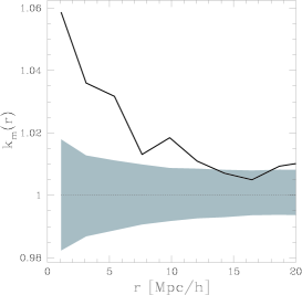
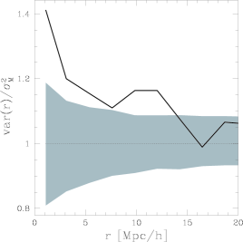
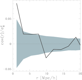
Figure 3: The luminosity-weighted correlation functions for a volume-limited subsample of the SSRS 2 with a depth of $100{{h^{-1}{\rm Mpc}}}$. The shaded areas denote the range of one-$\sigma$ fluctuations for randomized marks around the case of no mark segregation. The fluctuations were estimated from 1000 reshufflings of the luminosities.

The details of the mark correlation functions provide some further insight into the segregation effects. The mean mark $k_{m}(r)>1$ indicates that the luminous galaxies are more strongly clustered than the dim ones. Our signal is scale-dependent and decreasing for higher pair separations. The stronger clustering of luminous galaxies is in agreement with earlier claims comparing the correlation amplitude of several volume-limited samples kerscher_willmer:southern .
The ${{\text{{\it var}}}}(r)$ being larger than the mark variance of the whole sample, $\sigma^{2}_{M}$, shows that on galaxy pairs with separations smaller than $15{{h^{-1}{\rm Mpc}}}$ the luminosity fluctuations are enhanced. The fact that the mark segregation effect extends to scales of up to $15{{h^{-1}{\rm Mpc}}}$ is interesting on its own. In particular, it indicates that galaxy clusters are not the only source of luminosity segregation, since typically galaxy clusters are of the size of $3{{h^{-1}{\rm Mpc}}}$.
The signal for the covariance ${{\text{{\it cov}}}}(r)$, however, could be due to galaxy pairs inside clusters. It is relevant mainly on scales up to $4{{h^{-1}{\rm Mpc}}}$ indicating that the luminosities on galaxy pairs with small separations tend to assume similar values. – Our results in part confirm claims by kerscher_benoist:biasing , who compared the correlation functions $\xi_{2}$ for different volume-limited subsamples and different luminosity classes of the SSRS 2 catalog (see also kerscher_benoist:biasinghigher ).

0.2.2 Orientations of dark matter halos

Many structures found in the Universe such as galaxies and galaxy clusters show anisotropic features. Therefore one can assign orientations to them and ask whether these orientations are correlated and form coherent patterns. Here we discuss a similar question on the base of numerical simulations of large scale structure (e.g., kerscher_bertschinger:simulations ; kerscher_klypin:numericalI ).
In such simulations the trajectories of massive particles are numerically integrated. These particles represent the dominant mass component in the Universe, the dark matter. Through gravitational instability high density peaks (“halos”) form in the distribution of the particles; these halos are likely to be the places where galaxies originate. In the following we will report on alignment correlations between such halos kerscher_faltenbacher:halos , for a further application of mark correlation functions in this field see kerscher_gottloeber:merger .
The halos used by kerscher_faltenbacher:halos stem from a $N$-body simulation in a periodic box with a side length of 500$h^{-1}$Mpc. The initial and boundary conditions were fixed according to a $\Lambda$CDM cosmology (for a discussion of cosmological models see kerscher_peebles:principles ; kerscher_coles:cosmology ). Halos were identified using a friend-of-friends algorithm in the dark matter distribution. Not all of the halos found were taken into account; rather the mass range and the spatial number density of the selected halos were chosen to resemble the properties of observed galaxy clusters in the Reflex catalogue kerscher_boehringer:reflexI . Typically our halos show a prolate distribution of their dark matter particles.
For each halo the direction of the elongation is determined from the major axis of the mass-ellipsoid. This leads to a marked point set where the orientation ${\mathbf{l}}_{i}$ is attached to each halo position ${\mathbf{x}}_{i}$ as a vector mark with $|{\mathbf{l}}_{i}|=1$. Details can be founds in kerscher_faltenbacher:halos .
In Fig. 4 the vector-mark correlation functions as defined in Eqs. (14), (16), and (17) are shown. Since only the orientation of the mass ellipsoids can be determined, we use ${\cal A}^{\prime}(r)$ (Eq. 15) instead of ${\cal A}(r)$. The signal in ${\cal A}^{\prime}(r)$ indicates that pairs of halos with a distance smaller than 30$h^{-1}$Mpc  show a tendency of parallel alignment of their orientations ${\mathbf{l}}_{1},{\mathbf{l}}_{2}$. The deviation from a pure random alignment is in the percent range but clearly outside the random fluctuations. The alignment of the halos’ orientations ${\mathbf{l}}_{1},{\mathbf{l}}_{2}$ with the connecting vector $\hat{\mathbf{r}}$ quantified by ${\cal F}(r)$ is significantly stronger; it is particularly interesting that this alignment effect extends to scales of about 100$h^{-1}$Mpc.
In a qualitative picture this may be explained by halos aligned along the filaments of the large scale structure. Indeed such filaments are prominent features found in the galaxy distribution kerscher_huchra:cfa2s1 and in $N$-body simulations kerscher_melott:generation , often with a length of up to  100$h^{-1}$Mpc. The lowered ${\cal P}(r)$ indicates that the volume of the rhomboid given by ${\mathbf{l}}_{1},{\mathbf{l}}_{2}$ and $\hat{\mathbf{r}}$ is reduced for halo pairs with a separation below 80$h^{-1}$Mpc. Already a preferred alignment of ${\mathbf{l}}_{1},{\mathbf{l}}_{2}$ along $\hat{\mathbf{r}}$ leads to such a reduction, similar to a plane-like arrangement of ${\mathbf{l}}_{1},{\mathbf{l}}_{2},\hat{\mathbf{r}}$. For the halo distribution the signal in ${\cal P}(r)$ seems to be dominated by the filamentary alignment.

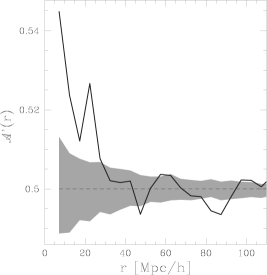
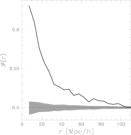
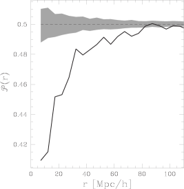
Figure 4: The correlations of halo orientations in numerical simulations. The orientation of each dark matter halo, specified by the direction of the major axis ${\mathbf{l}}$ of the mass ellipsoid, is used as a vector mark. The dashed area is obtained by randomizing the orientations among the halos.

The question whether there are non-trivial orientation patterns for galaxies or galaxy clusters has been discussed for a long time. kerscher_binggeli:shape reported a significant alignment of the observed galaxy clusters out to 100$h^{-1}$Mpc. kerscher_struble:new ; kerscher_struble:new-erratum , however claimed that this effect is small and likely to be caused by systematics; kerscher_ulmer:major find no indication for alignment effects at all. Subsequently several authors purported to have found signs of alignments in the galaxy and galaxy cluster distribution (see e.g. kerscher_djorgovski:coherent ; kerscher_lambas:statistics ; kerscher_fuller:alignments ; kerscher_heavens:intrinsic ). Our Fig. 4 shows that from simulations significant large-scale correlations are to be expected in the orientations of galaxy clusters, in agreement with the results by kerscher_binggeli:shape . These results are also supported by a simulation study carried out by kerscher_onuora:alignment .

0.2.3 Martian Craters

Let us now turn to another, still astrophysical, but significantly closer object: the Mars (see Figure 5). Many planets’ surfaces display impact craters with diameters up to $\sim 260\,$km and a broad range of inner morphologies. These craters are surrounded by ejecta forming different types of patterns. The craters and their ejecta are likely to be caused by asteroids and periodic comets crossing the planets’ orbits, falling down onto the planet’s surface, and spreading some of the underlying surfaces material around the original impact crater. A variety of different crater morphologies and a wide range of ejecta patterns can be found. In principle, either the different impact objects (especially their energies) or the various surface types of the planet may explain the repertory of patterns observed.

Figure 5: The Martian surface with its craters. Whereas the left panel (from http://pds.jpl.nasa.gov/planets/captions/mars/schiap.htm) illustrates the various geological settings to be found on the planet’s surface, the other panels focus on a small patch and show the craters together with their radii (middle panel, the size of the symbols are proportional to the radii of the craters) and together with the craters’ types (right panel, simple morphology as quadrangles and more complex craters as stars). The latter viewgraphs rely on the data by kerscher_barlow:martian .

Whereas the energy variations of impact objects do not cause any peculiarities in the spatial distribution of the craters (apart from a possible latitude dependence), geographic inhomogeneities are expected to originate inhomogeneities in the craters’ morphological properties.
We try to answer the question for the ejecta patterns’ origin using data collected by kerscher_barlow:martian who already found correlations between crater characteristics and the local surface type employing geologic maps of the Mars. Complementary to their approach, we investigate two-point properties without any reference to geologic Mars maps. We restrict ourselves only to craters which have a diameter larger than $8$ km and whose ejecta pattern could be classified, ending up with $3527$ craters spread out all over the Martian surface. We use spherical distances for our analysis of pairs.
In a first step we divide the ejecta patterns into two broad classes consisting of either the simple patterns (single and double lobe morphology, i.e. SL and DL in terms of the classification by kerscher_barlow:martian ; we speak of “simple craters”) or the remaining, more complex configurations (“complex craters”). Using our conditional cross correlation functions $C_{ij}$ as defined in Equation (8), we see a highly significant signal for mark correlations (Figure 6). At small separations, crater pairs are disproportionally built up of simple craters at the expense of cross correlations. This can be explained assuming that crater formation depends on the local surface type: if the simple craters are more frequent in certain geological environments than in others, then there are also more pairs of them to be found as far as one focuses on distances smaller than the typical scale of one geological surface type. Cross pairs are suppressed, since typical pairs with small separations belong to one geological setting where the simple craters either dominate or do not. Only a small, positive segregation signal occurs for the complex craters. Hence our analysis indicates that the broad class of complex craters is distributed quite homogeneously over all of the geologies. On top of this there are probably simple craters, their frequency significantly depending on the surface type.
If the ejecta patterns were independent of the surface, no mark segregation could be observed (other sources of mark segregation are unlikely, since the Martian craters are a result of a long bombardment history diluting any eventual peculiar crater correlations). In this sense, the signal observed indicates a surface-dependence of crater formation. This result is remarkable, given that we did not use any geological information on the Mars at all. The picture emerging could be described using the random field model, where a field (here the surface type) determines the mark of the points (see below).

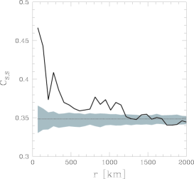
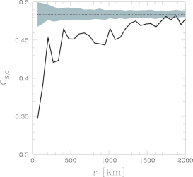
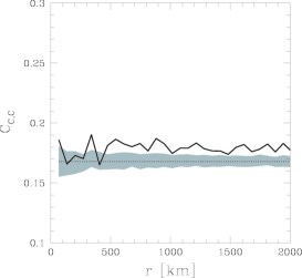
Figure 6: The conditional cross-correlation functions for Martian craters. We split the sample of craters into two broad classes according to their ejecta types: simple morphologies (S) consisting of SL and DL types, and complex morphologies (C) with all other types (see kerscher_barlow:martian for details). The results indicate, that at scales up to about $1500$ km the clustering of the simple craters is enhanced at expense of cross correlations. The shaded areas denote the one-$\sigma$ fluctuations for randomized marks estimated from 100 realizations of the mark reshuffling.

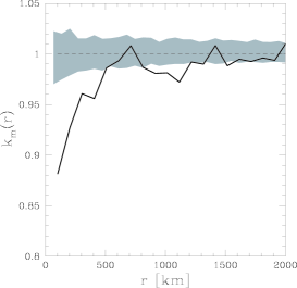
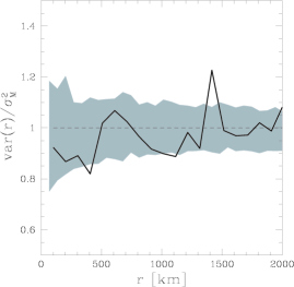
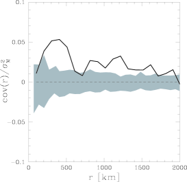
Figure 7: The radius-weighted correlation functions for craters on Mars. The radius of each crater serves as a mark. $r$ is the spherical distance. The shaded areas denote the one-$\sigma$ fluctuations for randomized marks estimated from 100 realizations of the mark reshuffling.

In a second step, we analyze the interplay between the craters’ diameters and their spatial clustering. Now the diameter serves as a continuous mark. The results in Figure 7 show a clear signal for mark segregation in $k_{m}$ and cov at small scales. The latter signals that pairs with separations in a broad range up to $1700$ km tend to have similar diameters; this is in agreement with the earlier picture: as kerscher_barlow:martian showed, the simple craters are mostly small-sized. Pairs with relatively small separations thus often stem from the same geological setting and therefore have similar diameters and similar morphological type.
Also the signal of $k_{m}$ seems to support this picture: since the simple craters are more strongly clustered than the other ones and since they have smaller diameters, one could expect $k_{m}<1$. As we shall see in Sect. 0.3, however, a $k_{m}\neq 1$ contradicts the random field model; therefore, the mark-dependence on the underlying surface type (thought of as a random field) cannot account for the signal observed. Thus, we have to look for an alternative explanation: it seems reasonable, that, whenever a crater is found somewhere, no other crater can be observed close nearby (because an impact close to an existing crater will either destroy the old one or cover it with ejecta such that it is not likely to be observed as a crater). This results in a sort of effective hard-core repulsion. This repulsion should be larger for larger craters. Thus, pairs with very small separations can only be formed by small craters, therefore $k_{m}<1$ for tiny $r$. The scale beyond which $k_{m}(r)\sim 1$ should somehow be hidden within the crater diameter distribution. Indeed, at about $500$ km the segregation vanishes, which is about twice the largest diameter in our sample. Taking into account that the ejecta patterns extend beyond the crater, this seems to be a reasonable agreement. As shown in Sect. 0.3.1 a model based on these consideration is able to produce such a depletion in the $k_{m}(r)$. This effect could also in turn explain part of the cross correlations observed earlier in Figure 6. A similar effect is to be expected for the mark variance. Close pairs are only accessible to craters with a smaller range of diameters; therefore, their variance is diminished in comparison to the whole sample. However, an effect like this is barely visible in the data.
Altogether, the crater distribution is dominated by two effects: the type of the ejecta pattern and the crater diameter depend on the surface, in addition, there is a sort of repulsion effect on small scales.

0.2.4 Pores in Sandstone

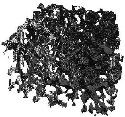
Figure 8: The pores within a Fontainbleau sandstone sample. Note, that this is a negative image, where the pores are displayed in grey. The geometrical features of the pore network are important for macroscopic properties of the stone. In this sample the pores occupy $13\%$ of the volume. The size of the whole sample shown is about $1.5$ mm³ (Courtesy M. Knackstedt).

Now we turn to systems on smaller scales. Sandstone is an example of a porous medium and has extensively been investigated, mainly because oil was found in the pore network of similar stones. In order to extract the oil from the stone one can try to wash it out using a second liquid, e.g. water. Therefore, one tries to understand from a theoretical point of view, how the microscopic geometry of the pore network determines the macroscopic properties of such a multi-phase flow. Especially the topology and connectivity of the microcaves and tunnels prove to be crucial for the flow properties at macroscopic scales. Details are given, for instance, in the contributions by C. Arns et al., H.-J. Vogel et al. and J. Ohser in this volume. A sensible physical model, therefore, in the first place has to rely on a thorough description of the pore pattern.
One way to understand the pore network is to think of it as a union of simple geometrical bodies. Following kerscher_sok:direct , one can identify distinct pores together with their position and their pore radius or extension. This allows us to understand the pore structure in terms of a marked point process, where the marks are the pore radii.
In the following, we consider three-dimensional data taken from one of the Fontainbleau sandstone samples through synchrotron X-ray tomography. These data trace a $4.52$ mm diameter cylindrical core extracted from a block with bulk porosity $\phi=13\%,$, where the bulk porosity is the volume fraction occupied by the pores. A piece with $2.91$mm length (resulting in a $46.7$ mm³ volume) of the core was imaged and tomographically reconstructed kerscher_flanery:thredimensional ; kerscher_spanne:synchrotron ; kerscher_arns:euler ; kerscher_arns:parallel . Further details of this sample are presented in the contribution by C. Arns et al. in this volume. Based on the reconstructed images the positions of pores and their radii were identified as described in kerscher_sok:direct .
In our results for the mark correlation functions a strong depletion of $k_{m}(r)$ and $var(r)$ is visible for $r<200\mu$m in Fig. 10.

Figure 9: The empirical one-point distribution ${\cal M}_{1}$ of the pore sizes.

This small-scale effect may be explained similarly to the Martian craters: large pores are never found close to each others, since they have to be separated by at least the sum of their radii. The histogram of the pore radii in Fig. 9 shows that most of the pores have radii smaller than 100$\mu$m, and consequently this effect is confined to $r<200\mu$m. In Sect. 0.3.1 we discuss the Boolean depletion model which is based on this geometric constraints and is able to produce such a reduction in the $k_{m}(r)$. This purely geometric constraint also explains the reduced $var(r)$ and increased covariance $cov(r)$.

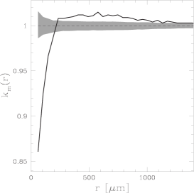
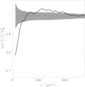
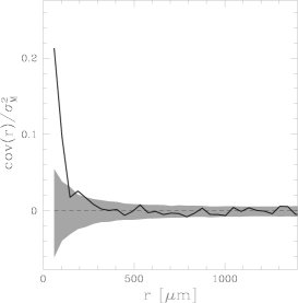
Figure 10: The mark-weighted correlation functions from the holes in the Fontainbleau sandstone. The pores’ radii serve as marks. The $k_{m}$ being smaller than one indicates a depletion effect. The shaded areas again denote the range of one-$\sigma$ fluctuations for randomized marks around the case of no mark segregation. The fluctuations were estimated from 200 reshufflings of the radii.

For separations larger than $200\mu$m there is no signal from the covariance, but both $k_{m}(r)$ and $var(r)$ show a small increase out to $\sim 1000\mu$m. This indicate that pairs of pores out to these separations tend to be larger in size and show slightly increased fluctuations. However, this effect is small (of the order of $1\%$) and may be explained by the definition of the holes, which may lead to “artificial small pores” as “bridges” between larger ones. This hypothesis has to be tested using different hole definitions. In any case the main conclusion seems to be that apart from the depletion effect at small scales there are no other mark correlations.

0.3 Models for marked point processes

Given the significant mark correlations found in various applications, one may ask how these signals can be understood in terms of stochastic models. A thorough understanding of course requires a physical modeling of the individual situation. There are, however, some generic models, which we will focus on in the following: in Sect. 0.3.1 we introduce the Boolean depletion model, which is able to explain some of the features observed in the distribution of craters and pores in sandstone. Another generic model is the random field model where the marks of the points stem from an independent random field (Section 0.3.2). In Sect. 0.3.3 we generalize the idea behind the random field model further in order to get the Cox random field model, which allows for correlations between the point set and the random field. Other model classes and their applications are discussed by e.g. kerscher_diggle:statistical ; kerscher_ogata:estimation ; kerscher_cressie:statistics ; kerscher_stoyan:fractals ; kerscher_waelder:models .

0.3.1 The Boolean depletion model

In our analysis of the Martian craters and the holes in sandstone, we found that for small separations only small craters, or small holes in the sandstone, could be found. We interpreted this as a pure geometric selection effect. The Boolean depletion model is able to quantify this effect, but also shows further interesting features.
The starting point is the Boolean model of overlapping spheres $B_{R}({\mathbf{x}})$ (see also the contributions by C. Arns et al. and D. Hug in this volume as well as kerscher_stoyan:lnp ). For that, the spheres’ centers ${\mathbf{x}}_{i}$ are generated randomly and independently, i.e. according to a Poisson process of number density $\varrho_{0}$. The radii $R$ of the spheres are then chosen independently according to a distribution function $F_{0}(R)$, i.e. with probability density $f_{0}(R)=\frac{\partial F_{0}(R)}{\partial R}$. The main idea behind the depletion is to delete spheres which are covered by other spheres. To make this procedure unique we remove only those spheres which are completely covered by a (notably larger) sphere. The positions and radii of the remaining spheres define a marked point process. Note, that this depletion mechanism is minimal in the sense that a lot of overlapping spheres may remain. This Boolean depletion model may be considered as the low-density limit of the well-known Widom-Rowlinson model, or (more generally) of non-additive hard sphere mixtures (see kerscher_widom:model ; kerscher_mecke:additivity ; kerscher_loewen:lnp ).
The probability that a sphere of radius $R$ is not removed is then given by

$$f_{\rm nr}(R) =\lim_{N,\Omega\rightarrow\infty}\prod_{i=1}^{N}\int_{0}^{\infty}{\rm d}R_{i}\ f_{0}(R_{i})\left(1-\frac{4\pi}{3}\frac{(R_{i}-R)^{3}}{|\Omega|}\Theta(R_{i}-R)\right)$$ (19)

$$=\exp\left(-\varrho_{0}\omega_{d}\int_{0}^{\infty}{\rm d}x\ f_{0}(R+x)x^{d}\right),$$ (20)

with the step function $\Theta(x)=0$ for $x<1$ and $\Theta(x)=1$ otherwise, and the volume of the $d$-dimensional unit ball $\omega_{d}$ ($\omega_{1}=2$, $\omega_{2}=\pi$, $\omega_{3}=4\pi/3$). The limit in Eq. (19) is performed by keeping $\varrho_{0}=N/|\Omega|$ constant, with $N$ the initial number of spheres and $|\Omega|$ the volume of the domain.
The number density of the remaining spheres reads

$$\varrho=\varrho_{0}\int_{0}^{\infty}{\rm d}R\ f_{0}(R)f_{\rm nr}(R)\;\;\;,$$ (21)

where the one-point probability density ${\cal M}_{1}(R)$ that a sphere has radius $R$ is given by

$${\cal M}_{1}(R)=f_{0}(R)f_{\rm nr}(R)\frac{\varrho_{0}}{\varrho}.$$ (22)

The probability that one or both of the spheres $B_{R_{1}}({\mathbf{x}}_{1})$ and $B_{R_{2}}({\mathbf{x}}_{2})$ are not removed is given by

$$f_{\rm nr}({\mathbf{x}}_{1},R_{1};{\mathbf{x}}_{2},R_{2})=\begin{cases}0&\text{if }r<|R_{2}-R_{1}|,\\ \exp\left(-\varrho_{0}g_{\rm nr}({\mathbf{x}}_{1},R_{1};{\mathbf{x}}_{2},R_{2})\right)&\text{otherwise },\end{cases}$$ (23)

with $B_{R<0}({\mathbf{x}})=\emptyset$ and

$$g_{\rm nr}({\mathbf{x}}_{1},R_{1};{\mathbf{x}}_{2},R_{2})=\int_{0}^{\infty}{\rm d}x\;V(B_{x-R_{1}}({\mathbf{x}}_{1})\cup B_{x-R_{2}}({\mathbf{x}}_{2}))\ f_{0}(x).$$ (24)

At this point we have to consider the set union of two spheres with radii $b_{1}\equiv x-R_{1}$ and $b_{2}\equiv x-R_{2}$, respectively; the volume of this geometrical configuration can be calculated; in three dimensions , e.g., we have:

$$V(B_{b_{1}}(\vec{x}_{1})\cup B_{b_{2}}(\vec{x}_{2})) =\frac{2\pi}{3}(b_{1}^{3}+b_{2}^{3})$$ (25)

$$\quad-\frac{2\pi}{3}\left(\frac{r^{3}}{8}-\frac{3}{4}r(b_{1}^{2}+b_{2}^{2})-\frac{3}{8r}(b_{2}^{2}-b_{2}^{2})^{2}\right)$$ (26)

for $|b_{2}-b_{1}|\leq r=|{\mathbf{x}}_{2}-{\mathbf{x}}_{2}|\leq b_{1}+b_{2}$. Otherwise this volume reduces either to the volume of the larger sphere ($r<|b_{2}-b_{1}|$) or to the sum of both spherical volumes ($r>b_{1}+b_{2}$).
Similarly as in Eq. (21) the spatial two-point density turns out to be

$$\varrho_{2}^{\cal S}({\mathbf{x}}_{1},{\mathbf{x}}_{2})=\varrho_{0}^{2}\int_{0}^{\infty}{\rm d}R_{1}\int_{0}^{\infty}{\rm d}R_{2}f_{0}(R_{1})f_{0}(R_{2})f_{\rm nr}({\mathbf{x}}_{1},R_{1};{\mathbf{x}}_{2},R_{2})\;\;\;,$$ (27)

such that the conditional two-point mark density simply reads

$${\cal M}_{2}(R_{1},R_{2}|{\mathbf{x}}_{1},{\mathbf{x}}_{2})=f_{0}(R_{1})f_{0}(R_{2})f_{\rm nr}({\mathbf{x}}_{1},R_{1};{\mathbf{x}}_{2},R_{2})\frac{\varrho_{0}^{2}}{\varrho_{2}^{\cal S}({\mathbf{x}}_{1},{\mathbf{x}}_{2})}.$$ (28)

From this we can derive all of the mark correlation functions from Sect. 0.1.4.

A bimodal distribution:

In order to get an analytically tractable model we adopt a bimodal radius distribution in the original Boolean model and start therefore with

$$f_{0}(R)=\alpha_{0}\delta(R-R_{1})+(1-\alpha_{0})\delta(R-R_{2})\;\;,$$ (29)

where we assume that $R_{1}<R_{2}$. Due to the depletion the number density $\varrho$ of the spheres as well as the probability $\alpha$ to find the smaller radius $R_{2}$ at a given point are then lowered; we get

$$\alpha =\alpha_{0}\frac{{\rm e}^{-n}}{1-\alpha_{0}+\alpha_{0}{\rm e}^{-n}}\leq\alpha_{0},$$ (30)

$$\varrho =\varrho_{0}\left(1-\alpha_{0}+\alpha_{0}{\rm e}^{-n}\right)=\varrho_{0}\frac{1-\alpha_{0}}{1-\alpha}$$ (31)

with $n=\varrho(1-\alpha)\frac{4\pi}{3}(R_{2}-R_{1})^{3}$. Altogether, the bimodal model can be parameterized in terms of the radii $R_{1}$ $R_{2}$, the ratio $\alpha_{0}\in[0,1]$ and the density $\varrho_{0}\in{\mathbf{R}}^{+}$. The latter two quantities, however are not observable from the final point process, therefore we convert them into the parameters $\alpha\in[0,1]$ and $\varrho\in{\mathbf{R}}^{+}$, so that all other quantities can be expressed in terms of these, for instance, $\alpha_{0}=\frac{\alpha}{\alpha+(1-\alpha){\rm e}^{-n}}\geq\alpha$, and $\varrho_{0}=\varrho\alpha{\rm e}^{n}+\varrho(1-\alpha)$,
From Eq. (22) we determine the mean mark, i.e. the mean radius of the spheres

$$\overline{m}=\overline{R}=\alpha R_{1}+(1-\alpha)R_{2},$$ (32)

and from Eq. (27) the spatial product density

$$\varrho_{2}^{\cal S}(r)=\varrho^{2}\begin{cases}(1-\alpha)^{2}R_{2}+\alpha^{2}R_{1}\exp\left(nI(x)\right)&0\leq x<1,\\[4.30554pt] 1+\alpha^{2}\left[\exp\left(nI(x)\right)-1\right]&1\leq x<2,\\[4.30554pt] 1&2\leq x,\end{cases}$$ (33)

with the normalized inter-sectional volume $I(x)=1-\frac{3}{4}x+\frac{1}{16}x^{3}$ of two spheres and $x=\frac{r}{|R_{2}-R_{1}|}$. Finally, using Eq. (28) one can calculate the mark correlation functions, e.g.

$$k_{m}(r)=\begin{cases}1-\alpha^{2}(1-\alpha)\frac{R_{2}-R_{1}}{\overline{R}}\frac{\exp\left(nI(x)\right)-\alpha^{-1}+1}{(1-\alpha)^{2}+\alpha^{2}\exp\left(nI(x)\right)}&0\leq x<1,\\[4.30554pt] 1-\alpha^{2}(1-\alpha)\frac{R_{2}-R_{1}}{\overline{R}}\frac{\exp\left(nI(x)\right)-1}{1+\alpha^{2}\left[\exp\left(nI(x)\right)-1\right]}&1\leq x<2,\\[4.30554pt] 1&2\leq x.\end{cases}$$ (34)

In Fig. 11 the $k_{m}(r)$ function from the Boolean depletion model is shown. The model with the solid line illustrates that a reduced $k_{m}(r)$ for small radii can be obtained by simply removing smaller spheres. At least qualitatively this model is able to explain the depletion effects we have seen both in the distribution of Martian craters (Fig. 7) and in the distribution of pores in sandstone (Fig. 10). The jump at $r=R_{2}-R_{1}$ is a relict of the strictly bimodal distribution with only two radii. Fig. 11 also shows that the Boolean depletion model is quite flexible, allowing for a $k_{m}(r)<1$, but also $k_{m}(r)>1$ is possible.
Without ignoring the considerable difference of this Boolean depletion model to the pore size distribution in real sandstones (see Figures 8-10) one may still recognize some interesting similarities: This simple model explains naturally a decrease of $k_{m}(r)$ if the distribution of the radii is symmetric ($\alpha=1/2$). As visible in Figure 9 this is approximately the case for the pore radii. Moreover, note that even quantitative features are captured correctly indicating that the decrease of $k_{m}(r)$ visible in Figure 10 is indeed due to a depletion effect. For instance, the decrease starts at $r\approx R_{M}$ where $R_{M}\approx 100\mu m$ is the largest occurring radius (see the histogram in Figure 9) and the value of $k_{m}(0)\approx 0.8$ at $r=0$ is in accordance with Equation (34) assuming that $R_{2}-R_{1}\approx\overline{R}$ and the normalized density of pores $n\approx 1$ necessary for a connected network. Of course a more detailed analysis is necessary based on Eqs. (22) and  (28) and the histogram shown in Figure 9.

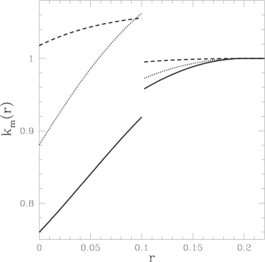
Figure 11: The $k_{m}(r)$ function for the Boolean depletion model with parameters $R_{1}=0.05$, $R_{2}=0.15$, $\varrho=500$, and $\alpha=0.5$ (solid line), $\alpha=0.3$ (dotted line), $\alpha=0.1$ (dashed line).

0.3.2 The random field model

The “random-field model” covers a class of models motivated from fields such as geology (see, e.g., kerscher_waelder:variograms ). The level of the ground water, for instance, is thought of as a realization of a random field which may be directly sampled at points (hopefully) independent from the value of the field or which may influence the size of a tree in a forest.
In general, a realization of the random field model is constructed from a realization of a point process and a realization of a random field $u({\mathbf{x}})$. The mark of each object located at ${\mathbf{x}}_{i}$ traces the accompanying random field via $m_{i}=u({\mathbf{x}}_{i})$. The crucial assumption is that the point process is stochastically independent from the random field.
We denote the mean value of the homogeneous random field by $\overline{u}={\mathbb{E}}[u({\mathbf{x}})]=\overline{u^{1}}$ and the moments by $\overline{u^{k}}=\int{\rm d}u\ w(u)u^{k}$, with the one-point probability density $w$ of the random field and ${\mathbb{E}}$ the expectation over realizations of the random field. The product density of the random field is $\rho_{2}^{u}(r)={\mathbb{E}}\big{[}u({\mathbf{x}}_{1})u({\mathbf{x}}_{2})\big{]}$ with $r=|{\mathbf{x}}_{1}-{\mathbf{x}}_{2}|$. For a general discussion of random field models, see kerscher_adler:randomfields .
In this model the one-point density of the marks is ${\cal M}_{1}(m)=w(m)$, and $\overline{m^{k}}=\overline{u^{k}}$ etc. The conditional mark density is given by

$${\cal M}_{2}(m_{1},m_{2}|{\mathbf{x}}_{1},{\mathbf{x}}_{2})={\mathbb{E}}\big{[}\delta(m_{1}-u({\mathbf{x}}_{1}))\delta(m_{2}-u({\mathbf{x}}_{2}))\big{]},$$ (35)

where $\delta$ is the Dirac delta distribution. Clearly, this expression is only well-defined under a suitable integral over the marks. With Eq. (7) one obtains

$$\left\langle m_{1}\right\rangle_{\rm P}(r)=\overline{u},\quad\left\langle m_{1}^{2}\right\rangle_{\rm P}(r)=\overline{u^{2}},\quad\left\langle m_{1}m_{2}\right\rangle_{\rm P}(r)=\rho_{2}^{u}(r),$$ (36)

and the mark-correlation functions defined in Sect. 0.1.4 read

$$k_{m}(r)=1,\ k_{mm}(r)=\rho_{2}^{u}(r)/\overline{u}^{2},\ \gamma(r)=\overline{u^{2}}-\rho_{2}^{u}(r),$$ (37)

$${{\text{{\it cov}}}}(r)=\rho_{2}^{u}(r)-\overline{u}^{2},\ {{\text{{\it var}}}}(r)=\overline{u^{2}}-\overline{u}^{2}=\sigma_{M}^{2}.$$ (38)

Therefore, there are some explicit predictions for the random field model: an empirically determined $k_{m}$ significantly differing from one not only indicates mark segregation, but also that the data is incompatible with the random field model. Looking at Figure 3 we see immediately that the galaxy data are not consistent with the random field model. Similar tests based on the relation between $k_{mm}$ and the mark-variogram $\gamma$ were investigated by kerscher_waelder:variograms and kerscher_schlather:characterization . The failure of the random field model to describe the luminosity segregation in the galaxy distribution allows the following plausible physical interpretation: the galaxies do not merely trace an independent luminosity field; rather the luminosities of galaxies depend on the clustering of the galaxies. We shall try to account for this with a better model in the following section.

0.3.3 The Cox random field model

In the random field model, the field was only used to generate the points’ marks. In the Cox random field model, on the contrary, the random field determines the spatial distribution of the points as well. As before, consider a homogeneous and isotropic random field $u({\mathbf{x}})\geq 0$. The point process is constructed as a Cox-process (see e.g. kerscher_stoyan:stochgeom ). The mean number of points in a set $B$ is given by the intensity measure

$$\Lambda(B)=\int_{B}{\rm d}{\mathbf{x}}\ a\ u({\mathbf{x}}),$$ (39)

where $a$ is a proportionality factor fixing the mean number density $\varrho=a\overline{u}$. The (spatial) product density of the point distribution is

$$\varrho_{2}^{\cal S}({\mathbf{x}}_{1},{\mathbf{x}}_{2})=a^{2}\ \rho_{2}^{u}(r)=a^{2}\ \overline{u}^{2}(1+\xi_{2}^{u}(r)),$$ (40)

where again $\rho_{2}^{u}(r)$ denotes the product density of the random field. $\xi_{2}^{u}$ is the normalized two-point cumulant of the random field (see below). We will also need the $n$-point densities of the random field:

$$\rho_{n}^{u}({\mathbf{x}}_{1},\ldots,{\mathbf{x}}_{n})={\mathbb{E}}\big{[}u({\mathbf{x}}_{1})\cdots u({\mathbf{x}}_{1})\big{]}.$$ (41)

Like in the random field model, the marks trace the field, but this time rather in a probabilistic way than in a deterministic one: the mark $m_{i}$ on a galaxy located at ${\mathbf{x}}_{i}$ is a random variable with the probability density $p(m_{i}|u({\mathbf{x}}_{i}))$ depending on the value of the field $u({\mathbf{x}}_{i})$ at ${\mathbf{x}}_{i}$. This can be used as a stochastic model for the genesis of galaxies depending on the local matter density.
In order to calculate the conditional mark correlation functions we define the conditional moments of the mark distribution given the value $u$ of the random field:

$$\overline{m^{k}}(u)=\int{\rm d}m\ p(m|u)\ m^{k}.$$ (42)

The spatial mark product-density is

$$\varrho_{2}^{SM}(({\mathbf{x}}_{1},m_{1}),({\mathbf{x}}_{2},m_{2}))=a^{2}{\mathbb{E}}\big{[}p(m_{1}|u({\mathbf{x}}_{1}))p(m_{2}|u({\mathbf{x}}_{2}))\ u({\mathbf{x}}_{1})u({\mathbf{x}}_{2})\big{]}.$$ (43)

and with Eq. (3)

$${\cal M}_{2}(m_{1},m_{2}|{\mathbf{x}}_{1},{\mathbf{x}}_{2})=\frac{1}{\rho_{2}^{u}(r)}{\mathbb{E}}\big{[}p(m_{1}|u({\mathbf{x}}_{1}))p(m_{2}|u({\mathbf{x}}_{2}))\ u({\mathbf{x}}_{1})u({\mathbf{x}}_{2})\big{]},$$ (44)

for $\rho_{2}^{u}(r)\neq 0$ and zero otherwise. The mark correlation functions can therefore be expressed in terms of weighted correlations of the random field:

$$\left\langle m\right\rangle_{\rm P}(r)=\frac{1}{\rho_{2}^{u}(r)}{\mathbb{E}}\big{[}\overline{m}(u({\mathbf{x}}_{1}))\ u({\mathbf{x}}_{1})u({\mathbf{x}}_{2})\big{]},$$ (45)

$$\left\langle m^{2}\right\rangle_{\rm P}(r)=\frac{1}{\rho_{2}^{u}(r)}{\mathbb{E}}\Big{[}\overline{m^{2}}(u({\mathbf{x}}_{1}))\ u({\mathbf{x}}_{1})u({\mathbf{x}}_{2})\Big{]},$$ (46)

$$\left\langle m_{1}m_{2}\right\rangle_{\rm P}(r)=\frac{1}{\rho_{2}^{u}(r)}{\mathbb{E}}\big{[}\overline{m}(u({\mathbf{x}}_{1}))\overline{m}(u({\mathbf{x}}_{2}))\ u({\mathbf{x}}_{1})u({\mathbf{x}}_{2})\big{]}.$$ (47)

A special choice for $p(m|u)$:

To proceed further, we have to specify $p(m|u)$. As a simple example we choose $m_{i}$ equal to the value of the field $u({\mathbf{x}}_{i})$ at the point ${\mathbf{x}}_{i}$, such as in the random field model. Thinking of the random field as a mass density field and the mark of a galaxy luminosity, that means that the galaxies trace the density field and that their luminosities are directly proportional to the value of the field. With $p(m|u)=\delta(m-u)$ the conditional mark moments become $\overline{m^{k}}(u)=u^{k}$. The moments of the unconstrained mark distribution read $\overline{m^{k}}=\overline{u^{k+1}}/\overline{u}$, and the three basic pair averages are

$$\left\langle m_{1}\right\rangle_{\rm P}(r)=\frac{\rho_{3}^{u}({\mathbf{x}}_{1},{\mathbf{x}}_{1},{\mathbf{x}}_{2})}{\rho_{2}^{u}(r)},\ \left\langle m_{1}^{2}\right\rangle_{\rm P}(r)=\frac{\rho_{4}^{u}({\mathbf{x}}_{1},{\mathbf{x}}_{1},{\mathbf{x}}_{1},{\mathbf{x}}_{2})}{\rho_{2}^{u}(r)}$$ (48)

$$\left\langle m_{1}m_{2}\right\rangle_{\rm P}(r)=\frac{\rho_{4}^{u}({\mathbf{x}}_{1},{\mathbf{x}}_{1},{\mathbf{x}}_{2},{\mathbf{x}}_{2})}{\rho_{2}^{u}(r)}.$$ (49)

Hence, the mark correlation functions defined in Sect. 0.1.4 are determined by the higher-order correlations of the random field. With the Cox random field model we go beyond the random field model, e.g.

$$k_{m}(r)=\frac{\left\langle m\right\rangle_{\rm P}(r)}{\overline{m}}=\frac{\overline{u}\ \rho_{3}^{u}({\mathbf{x}}_{1},{\mathbf{x}}_{1},{\mathbf{x}}_{2})}{\overline{u^{2}}\ \rho_{2}^{u}(r)}$$ (50)

is not equal to one any more.

Hierarchical field correlations:

At this point, we have to specify the correlations of the random field $u({\mathbf{x}})$. The simplest choice, a Gaussian random field, is not feasible here, since a number density (cp. Eq. 39) has to be strictly positive, whereas the Gaussian model allows for negative values. Instead, we will use the hierarchical ansatz: we first express the two- and three-point correlations in terms of normalized cumulants $\xi_{2}$ and $\xi_{3}$ (see, e.g., kerscher_daley:introduction ; kerscher_balian:I ; kerscher_kerscher:constructing ),

$$\rho_{2}^{u}({\mathbf{x}}_{1},{\mathbf{x}}_{2})=\overline{u}^{2}\Big{(}1+\xi_{2}^{u}({\mathbf{x}}_{1},{\mathbf{x}}_{2})\Big{)},\\ \rho_{3}^{u}({\mathbf{x}}_{1},{\mathbf{x}}_{2},{\mathbf{x}}_{3})=\overline{u}^{3}\Big{(}1+\xi_{2}^{u}({\mathbf{x}}_{1},{\mathbf{x}}_{2})+\xi_{2}^{u}({\mathbf{x}}_{2},{\mathbf{x}}_{3})+\xi_{2}^{u}({\mathbf{x}}_{1},{\mathbf{x}}_{3})+\xi_{3}^{u}({\mathbf{x}}_{1},{\mathbf{x}}_{2},{\mathbf{x}}_{3})\Big{)}.$$ (51)

In order to eliminate $\xi_{3}^{u}$ we use the hierarchical ansatz (see e.g. kerscher_peebles:lss ):

$$\xi_{3}^{u}({\mathbf{x}}_{1},{\mathbf{x}}_{2},{\mathbf{x}}_{3})=Q\Big{(}\xi_{2}^{u}({\mathbf{x}}_{1},{\mathbf{x}}_{2})\xi_{2}^{u}({\mathbf{x}}_{2},{\mathbf{x}}_{3})+\xi_{2}^{u}({\mathbf{x}}_{2},{\mathbf{x}}_{3})\xi_{2}^{u}({\mathbf{x}}_{1},{\mathbf{x}}_{3})\\ +\xi_{2}^{u}({\mathbf{x}}_{1},{\mathbf{x}}_{2})\xi_{2}^{u}({\mathbf{x}}_{1},{\mathbf{x}}_{3})\Big{)}.$$ (52)

This ansatz is in reasonable agreement with data from the galaxy distribution, provided $Q$ is of the order of unity (kerscher_szapudi:higherapm ). Several choices for $\xi_{2}(r)$ and $Q$ lead to well-defined Cox point process models based on the random field $u({\mathbf{x}})$ kerscher_balian:I ; kerscher_szapudi:higher . Now we can express $k_{m}(r)$ from Eq. (50) entirely in terms of the two-point correlation function $\xi_{2}^{u}(r)$ of the random field:

$$k_{m}(r)=\frac{1+2\xi_{2}^{u}(r)+\xi_{2}^{u}(0)+Q\Big{(}\xi_{2}^{u}(r)^{2}+2\xi_{2}^{u}(r)\xi_{2}^{u}(0)\Big{)}}{\Big{(}1+\xi_{2}^{u}(r)\Big{)}\Big{(}1+\xi_{2}^{u}(0)\Big{)}},$$ (53)

where we made use of the fact that $\sigma_{u}^{2}=\overline{u^{2}}-\overline{u}^{2}=\overline{u}^{2}\xi_{2}^{u}(0)$. Inserting typical parameters found from the spatial clustering of the galaxy distribution we see from Fig. 12 that the Cox random field model allows us to qualitatively describe the observed luminosity segregation in Fig.3. But the amplitude of $k_{m}$ predicted by this model is too high. The Cox random field model, however, is quite flexible in allowing for different choices for $p(m|u)$; also different models for the higher-order correlations of the random field may be used, e.g.  a log-normal random field kerscher_coles:lognormal ; kerscher_moller:log . Clearly more work is needed to turn this into viable model for the galaxy distribution.

Figure 12: The $k_{m}(r)$ function for the Cox random field model according to Eq. (53). We use $Q=1$ and $\xi_{2}^{u}(r)=(5{{h^{-1}{\rm Mpc}}}/r)^{1.7}$ truncated on small scales at $\xi_{2}^{u}(r<0.1{{h^{-1}{\rm Mpc}}})=\sigma_{u}^{2}/\overline{u}^{2}=\xi_{2}^{u}(0)\sim 750$.

0.4 Conclusions

Whenever objects are sampled together with their spatial positions and some of their intrinsic properties, marked point processes are the stochastic models for those data sets. Combining the spatial information and the objects’ inner properties one can constrain their generation mechanism and their interactions.
Developing the framework of marked point processes further and outlining some of their general notions is thus of interest for physical applications. Let us therefore look at mark correlations again from both a statistical and a physical perspective. We focused on two kinds of dependencies.
On the one hand, one can always ask, whether objects of different types “know” from each other. From a statistical point of view, this is the question whether the marked point process consists of two completely independent sub-point processes. Physically, this concerns the question whether the objects have been generated together and whether they interact with each other.
On the other hand, it is often interesting to know whether the spatial distribution of the objects changes with their inner properties. For the statistician, this translates into the question whether mark segregation or mark-independent clustering is present. For the physicist such a dependency is interesting since one can learn from them whether and how the interactions distinguish between different object classes or whether the formation of the objects’ mark depends on the environment.
We discussed statistics capable of probing to which extent mark correlations are present in a given data set, and showed how to assess the statistical significance. Applying our statistics to real data, we could demonstrate, that the clustering of galaxies depends on their luminosities. Large scale correlations of the orientations of dark matter halos were found. Using the Mars data we could validate a picture of crater generation on the Martian surface: mainly, the local geological setting determines the crater type. We also could show that the sizes of pores in sandstone are correlated.
In order to understand empirical data sets in detail, we need models to compare to. As generic models the Boolean depletion model, the random field model and its extension, the Cox random field models are of interest.
Further application of the mark correlations properties may inspire the development of further models. It seems therefore that marked point processes could spark interesting interactions between physicists and mathematicians. Certainly, the distributions of physicists and mathematicians in coffee breaks at the Wuppertal conference were clustered, each. But could one observe positive cross-correlations? Using mark correlations we argue, that, even more, there is lots of space for positive interactions.….

Acknowledgments

We would like to thank Andreas Faltenbacher, Stefan Gottlöber and Volker Müller for allowing us to present some results from the orientation analysis of the dark matter halos (Sect. 0.2.2). For providing the sandstone data (Sect. 0.2.4) and discussion we thank Mark Knackstedt. Herbert Wagner provided constant support and encouragement, especially we would like to thank him for introducing us to the concepts of geometric algebra as used in the Appendix.

Appendix: Completeness of mark correlation functions

In order to form versatile test functions for describing mark segregation effects, we integrated the conditional mark probability density ${\cal M}_{2}(m_{1},m_{2}|r)$ twice in mark space thereby weighting with a function of the marks $f(m_{1},m_{2})$ (see Eq. 7). Such a pair-averaging reduces the full information present in ${\cal M}_{2}(m_{1},m_{2}|r)$. So one may ask, whether or in which sense the mark correlation functions give a complete picture of the present two-point mark correlations.
For scalar marks $m_{i}$ this task is trivial. With a polynomial weighting function $f(m_{1},m_{2})\sim m_{1}^{n_{1}}m_{2}^{n_{2}}$ ($n_{1},n_{2}=0,1,..$) we consider moments of ${\cal M}_{2}(m_{1},m_{2}|r)$, hence, we can be complete only up to a given polynomial order in the marks $m_{1}$ and $m_{2}$. At first order there is only the mean $\left\langle m\right\rangle_{\rm P}(r)$. At second order we have $\left\langle m^{2}\right\rangle_{\rm P}(r)$ and $\left\langle m_{1}m_{2}\right\rangle_{\rm P}(r)$. All the mark correlation functions discussed in Sect. 0.1.4 can be constructed from these three pair averages. Higher-order moments of the marks involve more and more cross-terms.
For vector-valued marks, however, it is not obvious that the test quantities proposed in Sect. 0.1.4 trace all possible correlations between the vectors up to third order. To settle this case we have to consider the framework of geometric algebra, also called Clifford algebra. A detailed introduction to geometric algebra is given in kerscher_hestens:new , shorter introductions are kerscher_gull:imaginary ; kerscher_lasenby:unified . In geometric algebra one assigns a unique meaning to the geometric product (or Clifford product) of quantities like vectors, directed areas, directed volumes, etc. The geometric product ${\mathbf{a}}{\mathbf{b}}$ of two vectors ${\mathbf{a}}$ and ${\mathbf{b}}$ splits into its symmetric and antisymmetric part

$${\mathbf{a}}{\mathbf{b}}={\mathbf{a}}\cdot{\mathbf{b}}+{\mathbf{a}}\wedge{\mathbf{b}}.$$ (54)

Here ${\mathbf{a}}\cdot{\mathbf{b}}$ denotes the usual scalar product; in three dimensions, the wedge product ${\mathbf{a}}\wedge{\mathbf{b}}$ is closely related to the cross product between these two vectors. However, ${\mathbf{a}}\wedge{\mathbf{b}}$ is not a vector like ${\mathbf{a}}\times{\mathbf{b}}$, but a bivector – a directed area. Higher products of vectors can be simplified according to the rules of geometric algebra (for details see kerscher_hestens:new ).
Let us consider the situation where objects situated at ${\mathbf{x}}_{1}$ and ${\mathbf{x}}_{2}$ bear vector marks ${\mathbf{l}}_{1}$ and ${\mathbf{l}}_{2}$, respectively, and let the normalized distance vector be $\hat{\mathbf{r}}=({\mathbf{x}}_{1}-{\mathbf{x}}_{2})/r$. Note, that $\hat{\mathbf{r}}$ is not a mark at all, rather it can be thought of as another vector which may be useful for constructing mark correlation functions.
For many applications it is reasonable to assume isotropy in mark space, i.e. all of the mark correlation functions are invariant under common rotations of the marks. For galaxies, e.g., there does not seem to be an a priori preferred direction for their orientation. In more detail we have then

$$\begin{split}{\cal M}_{1}({\mathbf{l}})&={\cal M}_{1}(R{\mathbf{l}})={\cal M}_{1}(|{\mathbf{l}}|)\;\;\;,\\ {\cal M}_{2}({\mathbf{l}}_{1},{\mathbf{l}}_{2}|r)&={\cal M}_{2}(R{\mathbf{l}}_{1},R{\mathbf{l}}_{2}|r)\;\;\;,\end{split}$$ (55)

and so on, where $R$ is an arbitrary rotation in mark space. This means that the mark correlation functions depend only on rotationally invariant combinations of the vector marks. Therefore, only rotationally invariant combinations of vectors are sensible building blocks for weighting functions. We thus can restrict ourselves to scalar weighting functions, which result in coordinate-independent vector-mark correlation functions.
Again we proceed by considering mixed moments as basic combinations. We restrict ourselves to scalar quantities being polynomial in the vector components. One may also discuss moments in a broader sense allowing for vector moduli. In this wider sense, for example, $|{\mathbf{l}}_{1}|$ or $|{\mathbf{l}}_{1}\times({\mathbf{l}}_{1}\times\hat{\mathbf{r}})|$ would be allowed. We do not consider such quantities here, because they are not polynomial in the vector components. Their squares anyway appear at higher orders. Furthermore, it turns out that the characterization we will provide depends on the embedding dimension. The first- and second-order moments are identical in two and three dimensions, but at the third order they start to differ.

1. In the strict sense of scalar quantities being linear in the vector components there are no first-order moments for vectors.

2. At second order we encounter the following products: ${\mathbf{l}}_{1}{\mathbf{l}}_{1}$, $\hat{\mathbf{r}}\hat{\mathbf{r}}$, ${\mathbf{l}}_{1}{\mathbf{l}}_{2}$, $\hat{\mathbf{r}}{\mathbf{l}}_{1}$. Note, that, e.g., ${\mathbf{l}}_{1}\hat{\mathbf{r}}$ and ${\mathbf{l}}_{2}\hat{\mathbf{r}}$ do not make any difference as regards the mark correlation functions, since the pair averages implicitly render the indices symmetric; moreover, although the geometrical product is non-commutative, ${\mathbf{l}}_{1}\wedge\hat{\mathbf{r}}$ and ${\mathbf{l}}_{1}\wedge\hat{\mathbf{r}}$ do not lead to different mark correlation functions. Furthermore, $\hat{\mathbf{r}}\hat{\mathbf{r}}=1$. ${\mathbf{l}}_{1}{\mathbf{l}}_{1}={\mathbf{l}}_{1}\cdot{\mathbf{l}}_{1}=l_{1}^{2}$ provides us with higher moments of the modulus of the vectors. To investigate these kinds of correlations already scalar marks would be sufficient. New information is encoded in the other products.
   Consider ${\mathbf{l}}_{1}{\mathbf{l}}_{2}={\mathbf{l}}_{1}\cdot{\mathbf{l}}_{2}+{\mathbf{l}}_{1}\wedge{\mathbf{l}}_{2}$. The symmetric part ${\mathbf{l}}_{1}\cdot{\mathbf{l}}_{2}$ is clearly a scalar and defines the alignment ${\cal A}(r)$ (Eq. 14). The antisymmetric part ${\mathbf{l}}_{1}\wedge{\mathbf{l}}_{2}$ is a bivector. Its – unique – modulus (see again kerscher_hestens:new ), $|{\mathbf{l}}_{1}\wedge{\mathbf{l}}_{2}|=\sqrt{l_{1}^{2}l_{2}^{2}-({\mathbf{l}}_{1}\cdot{\mathbf{l}}_{2})^{2}}$, may be useful, but is no longer a polynomial in the vector components. $|{\mathbf{l}}_{1}\wedge{\mathbf{l}}_{2}|^{2}$ appears at the fourth order. In a completely analogous way we can treat ${\mathbf{l}}_{1}\hat{\mathbf{r}}={\mathbf{l}}_{1}\cdot\hat{\mathbf{r}}+{\mathbf{l}}_{1}\wedge\hat{\mathbf{r}}$. The symmetric part ${\mathbf{l}}_{1}\cdot\hat{\mathbf{r}}$ defines ${\cal F}(r)$. Hence at second order, the only possible vector-mark correlation functions are ${\cal A}(r)$ and ${\cal F}(r)$.

3. At third order we have to consider products of three vectors. In general the product of three vectors ${\mathbf{a}},{\mathbf{b}},{\mathbf{c}}$ splits into

   $${\mathbf{a}}{\mathbf{b}}{\mathbf{c}}={\mathbf{a}}({\mathbf{b}}\cdot{\mathbf{c}})+({\mathbf{a}}\cdot{\mathbf{b}}){\mathbf{c}}-({\mathbf{a}}\cdot{\mathbf{c}}){\mathbf{b}}+{\mathbf{a}}\wedge({\mathbf{b}}\wedge{\mathbf{c}}).$$ (56)

   i.e., a vector (consisting of the three first terms), and a pseudo-scalar, a directed volume. In two dimensions the pseudo-scalar ${\mathbf{a}}\wedge({\mathbf{b}}\wedge{\mathbf{c}})$ vanishes.
   Now we have to form all possible products of the three vectors ${\mathbf{l}}_{1},{\mathbf{l}}_{2},\hat{\mathbf{r}}$ and to derive scalars. In three dimensions the only new combination is the pseudo-scalar ${\mathbf{l}}_{1}\wedge({\mathbf{l}}_{2}\wedge\hat{\mathbf{r}})$ giving the oriented volume ${\mathbf{l}}_{1}\cdot({\mathbf{l}}_{2}\times\hat{\mathbf{r}})$. Unfortunately, this oriented volume averages out to zero. Thus, in a strict sense, there are no interesting third-order quantities. Closely related, however, is the modulus of the pseudoscalar $|{\mathbf{l}}_{1}\cdot({\mathbf{l}}_{2}\times\hat{\mathbf{r}})|$ proportional to our ${\cal P}(r)$. This expression is invariant under permutations of the vectors.

4. At third order and in two dimensions all of the relevant combinations are products of first- and second-order combinations; no specifically new combination appears. This is different from the case of three dimensions, where at third order an entirely new geometric object, the pseudo-scalar ${\mathbf{l}}_{1}\wedge({\mathbf{l}}_{2}\wedge\hat{\mathbf{r}})$ can be constructed. There is a general scheme behind this argument: since in $d$ dimensions any geometrical product of more than $d$ vectors vanishes, all relevant combinations of vectors at orders higher than $d$ are essentially products of combinations of lower-order factors.

References

- (1)
- (2) Adler, R. J. (1981): The Geometry of Random Fields (John Wiley & Sons, Chichester)
- (3) Arns, C., M. Knackstedt, W. Pinczewski, K. Mecke (2001): ’Characterisation of irregular spatial structures by prallel sets’, In press
- (4) Arns, C., M. Knackstedt, W. Pinczewski, K. Mecke (2001): ’Euler-poincaré characteristics of classes of disordered media’, Phys. Rev. E 63, p. 31112
- (5) Baddeley, A. J. (1999): ’Sampling and censoring’. In: Stochastic Geometry, Likelihood and Computation, ed. by O. Barndorff-Nielsen, W. Kendall, M. van Lieshout, volume 80 of Monographs on Statistics and Applied Probability, chapter 2 (Chapman and Hall, London)
- (6) Balian, R., R. Schaeffer (1989): ’Scale–invariant matter distribution in the Universe I. counts in cells’, Astronomics & Astrophysics 220, pp. 1–29
- (7) Barlow, N. G., T. L. Bradley (1990): ’Martian impact craters: Correlations of ejecta and interior morphologies with diameter, latitude, and terrain’, Icarus 87, pp. 156–179
- (8) Beisbart, C., M. Kerscher (2000): ’Luminosity– and morphology–dependent clustering of galaxies’, Astrophysical Journal 545, pp. 6–25
- (9) Benoist, C., A. Cappi, L. Da Costa, S. Maurogordato, F. Bouchet, R. Schaeffer (April 1999): ’Biasing and high-order statistics from the southern-sky redshift survey’, Astrophysical Journal 514, pp. 563–578
- (10) Benoist, C., S. Maurogordato, L. Da Costa, A. Cappi, R. Schaeffer (December 1996): ’Biasing in the galaxy distribution’, Astrophysical Journal 472, p. 452
- (11) Bertschinger, E. (1998): ’Simulations of structure formation in the universe’, Ann. Rev. Astron. Astrophys. 36, pp. 599–654
- (12) Binggeli, B. (1982): ’The shape and orientation of clusters of galaxies’, Astronomics & Astrophysics 107, pp. 338–349
- (13) Böhringer, H., P. Schuecker, L. Guzzo, C. Collins, W. Voges, S. Schindler, D. Neumann, G. Chincharini, R. Cruddace, A. Edge, H. MacGillivray, P. Shaver (2001): ’The ROSTA-ESO flux limited X-ray (REFLEX) galaxy cluster survey I: The construction of the cluster sample’, Astronomics & Astrophysics , p. 826
- (14) Capobianco, R., E. Renshaw (1998): ’The autocovariance function of marked point processes: A comparison between two different approaches’, Biom. J. 40, pp. 431–446
- (15) Coles, P., B. Jones (January 1991): ’A lognormal model for the cosmological mass distribution’, MNRAS 248, pp. 1–13
- (16) Coles, P., F. Lucchin (1994): Cosmology: The Origin and Evolution of Cosmic Structure (John Wiley & Sons, Chichester)
- (17) Cox, D., V. Isham (1980): Point Processes (Chapman and Hall, London)
- (18) Cressie, N. (1991): Statistics for Spatial Data (John Wiley & Sons, Chichester)
- (19) da Costa, L. N., C. N. A. Willmer, P. Pellegrini, O. L. Chaves, C. Rite, M. A. G. Maia, M. J. Geller, D. W. Latham, M. J. Kurtz, J. P. Huchra, M. Ramella, A. P. Fairall, C. Smith, S. Lipari (1998): ’The Southern Sky Redshift Survey’, AJ 116, pp. 1–7
- (20) Daley, D. J., D. Vere-Jones (1988): An Introduction to the Theory of Point Processes (Springer, Berlin)
- (21) Diggle, P. J. (1983): Statistical Analysis of Spatial Point Patterns (Academic Press, New York and London)
- (22) Djorgovski, S. (1987): ’Coherent orientation effects of galaxies and clusters’. In: Nearly Normal Galaxies. From the Planck Time to the Present, ed. by S. M. Faber (Springer, New York), pp. 227–233
- (23) Faltenbacher, A., S. Gottlöber, M. Kerscher, V. Müller (2002): ’Spin and orientational correlations of halos’, In preparation
- (24) Flannery, B. P., H. W. Deckman, W. G. Roberge, K. L. D’amico (1987): ’Three–dimensional X–ray microtomography’, Science 237, pp. 1439–1444
- (25) Fuller, T. M., M. J. West, T. J. Bridges (1999): ’Alignments of the dominant galaxies in poor clusters’, Astrophysical Journal 519, pp. 22–26
- (26) Gottlöber, S., M. Kerscher, A. Klypin, A. Kravtsov, V. Müller, A. Faltenbacher (2002): ’Spatial distribution of galactic halos and their merger histories’, In preparation
- (27) Gull, S., A. Lasenby, C. Doran (1993): ’Imaginary numbers are nor real. – the geometric algebra of spacetime’, Found. Phys. 23(9), p. 1175
- (28) Guzzo, L., J. Bartlett, A. Cappi, S. Maurogordato, E. Zucca, G. Zamorani, C. Balkowski, A. Blanchard, V. Cayatte, G. Chincarini, C. Collins, D. Maccagni, H. MacGillivray, R. Merighi, M. Mignoli, D. Proust, M. Ramella, R. Scaramella, G. Stirpe, G. Vettolani (2000): ’The ESO Slice Project (ESP) galaxy redshift survey. VII. the redshift and real-space correlation functions’, Astronomics & Astrophysics 355, pp. 1–16
- (29) Hamilton, A. J. S. (August 1988): ’Evidence for biasing in the cfa survey’, Astrophysical Journal 331, pp. L59–L62
- (30) Heavens, A. F., A. Refregier, C. Heymans (2000): ’Intrinsic correlation of galaxy shapes: implications for weak lensing measurements’, MNRAS 319, pp. 649–656
- (31) Hermit, S., B. X. Santiago, O. Lahav, M. A. Strauss, M. Davis, A. Dressler, J. P. Huchra (1996): ’The two–point correlation function and the morphological segregation in the optical redshift survey’, MNRAS 283, p. 709
- (32) Hestens, D. (1986): New Foundations for Classical Mechanics (D. Reidel Publishing Company, Dordrecht, Holland)
- (33) Huchra, J. P., M. J. Geller, V. De Lapparent, H. G. Corwin Jr. (1990): ’The CfA redshift survey – data for the NGP + 30 zone’, ApJS 72, pp. 433–470
- (34) Isham, V. (1985): ’Marked point processes and their correlations’. In: Spatial Processes and Spatial Time Series Analysis, ed. by F. Droesbeke (Publications des Facultés universitaires Sain-Louis, Bruxelles)
- (35) Kerscher, M. (2000): ’Statistical analysis of large–scale structure in the Universe’. In: Statistical Physics and Spatial Statistics: The Art of Analyzing and Modeling Spatial Structures and Pattern Formation, ed. by K. R. Mecke, D. Stoyan, Number 554 in Lecture Notes in Physics (Springer, Berlin), astro-ph/9912329
- (36) Kerscher, M. (2001): ’Constructing, characterizing and simulating Gaussian and high–order point processes’, Phys. Rev. E 64(5), p. 056109, astro-ph/0102153
- (37) Klypin, A. A. (2000): ’Numerical simulations in cosmology i: Methods’, in ’Lecture at the Summer School ”Relativistic Cosmology: Theory and Observations”’, Astro-ph/0005502
- (38) Lambas, D. G., E. J. Groth, P. Peebles (1988): ’Statistics of galaxy orientations: Morphology and large–scale structure’, AJ 95, pp. 975–984
- (39) Lasenby, J., A. N. Lasenby, C. J. Doran (2000): ’A unified mathematical language for physics and engineering in the 21st century’, Phil. Trans. R. Soc. London A 358, pp. 21–39
- (40) Löwen, H. (2000): ’Fun with hard spheres’. In: Statistical Physics and Spatial Statistics: The Art of Analyzing and Modeling Spatial Structures and Pattern Formation, ed. by K. R. Mecke, D. Stoyan, Number 554 in Lecture Notes in Physics (Springer, Berlin)
- (41) Mecke, K. (2000): ’Additivity, convexity, and beyond: Application of minkowski functionals in statistical physics’. In: Statistical Physics and Spatial Statistics: The Art of Analyzing and Modeling Spatial Structures and Pattern Formation, ed. by K. R. Mecke, D. Stoyan, Number 554 in Lecture Notes in Physics (Springer, Berlin)
- (42) Melott, A. L., S. F. Shandarin (1990): ’Generation of large-scale cosmological structures by gravitational clustering’, Nature 346, pp. 633–635.
- (43) Møller, J., A. R. Syversveen, R. P. Waagepetersen (1998): ’Log Gaussian cox processes’, Scand. J. Statist. 25, pp. 451–482
- (44) Ogata, Y., K. Katsura (1988): ’Likelihood analysis of spatial inhomogeneity for marked point pattersn’, Ann. Inst. Statist. Math. 40, pp. 29–39
- (45) Ogata, Y., M. Tanemura (1985): ’Estimation of interaction potentials of marked spatial point patterns through the maximum likelihood method’, Biometrics 41, pp. 421–433
- (46) Ohser, J., D. Stoyan (1981): ’On the second–order and orientation analysis of planar stationary point processes’, Biom. J. 23, pp. 523–533
- (47) Onuora, L. I., P. A. Thomas (2000): ’The alignment of clusters using large–scale simulations’, MNRAS 319, pp. 614–618
- (48) Peebles, P. J. E. (1980): The Large Scale Structure of the Universe (Princeton University Press, Princeton, New Jersey)
- (49) Peebles, P. J. E. (1993): Principles of Physical Cosmology (Princeton University Press, Princeton, New Jersey)
- (50) Penttinen, A., D. Stoyan (1989): ’Statistical analysis for a class of line segment processes’, Scand. J. Statist. 16, pp. 153–168
- (51) Reichert, H., O. Klein, H. Dosch, M. Denk, V. Honkimäki, T. Lippmann, G. Reiter (2000): ’Observation of five-fold local symmetry in liquid lead’, Nature 408, p. 839
- (52) Schlather, M. (2001): ’On the second–order characteristics of marked point processes’, Bernoulli 7(1), pp. 99–107
- (53) Schlather, M. (2002): ’Characterization of point processes with Gaussian marks independent of locations’, Math. Nachr. Accepted
- (54) Sok, R. M., M. A. Knackstedt, A. P. Sheppard, W. V. Pinczewski, W. B. Lindquist, A. V. A, , L. Paterson (2000): ’Direct and stochastic generation of network models from tomographic images; effect of topology on two-phase flow properties’. In: Proc. Upscaling Downunder, ed. by L. Paterson, (Kluwer Academic, Dordrecht)
- (55) Spanne, P., J. Thovert, C. Jacquin, W. Lindquist, K. Jones, P. Adler (1994): ’Synchrotron computed microtomography of porous media: Topology and transport’, Phys. Rev. Lett. 73, pp. 2001–2004
- (56) Stoyan, D. (1984): ’On correlations of marked point processes’, Math. Nachr. 116, pp. 197–207
- (57) Stoyan, D. (2000): ’Basic ideas of spatial statistics’. In: Statistical Physics and Spatial Statistics: The Art of Analyzing and Modeling Spatial Structures and Pattern Formation, ed. by K. R. Mecke, D. Stoyan, Number 554 in Lecture Notes in Physics (Springer, Berlin)
- (58) Stoyan, D. (2000): ’Recent applications of point process methods in forestry statistics’, Statistical Sciences 15, pp. 61–78
- (59) Stoyan, D., W. S. Kendall, J. Mecke (1995): Stochastic Geometry and its Applications (John Wiley & Sons, Chichester), 2nd edition
- (60) Stoyan, D., H. Stoyan (1985): ’On one of matérn’s hard-core point process models’, Biom. J. 122, p. 205
- (61) Stoyan, D., H. Stoyan (1994): Fractals, Random Shapes and Point Fields (John Wiley & Sons, Chichester)
- (62) Stoyan, D., O. Wälder (2000): ’On variograms in point process statistics, ii: Models for markings and ecological interpretation’, Biom. J. 42, pp. 171–187
- (63) Struble, M. F., P. Peebles (1985): ’Erratum: A new application of Binggeli’s test for large–scale alignment of clusters of galaxies’, AJ 90, pp. 582–589
- (64) Struble, M. F., P. Peebles (1986): ’A new application of binggeli’s test for large–scale alignment of clusters of galaxies’, AJ 91, p. 1474
- (65) Sylos Labini, F., M. Montuori, L. Pietronero (1998): ’Scale invariance of galaxy clustering’, Physics Rep. 293, pp. 61–226
- (66) Szapudi, I., G. B. Dalton, G. Efstathiou, A. S. Szalay (1995): ’Higher order statistics from the APM galaxy survey’, Astrophysical Journal 444, pp. 520–531
- (67) Szapudi, I., A. S. Szalay (1993): ’Higher order statistics of the galaxy distribution using generating functions’, Astrophysical Journal 408, pp. 43–56
- (68) Ulmer, M., S. L. W. McMillan, M. P. Kowalski (1989): ’Do the major axis of rich clusters of galaxies point toward their neighbors?’, Astrophysical Journal 338, pp. 711–717
- (69) van Lieshout, M. N. M., A. J. Baddeley (1996): ’A nonparametric measure of spatial interaction in point patterns’, Statist. Neerlandica 50, pp. 344–361
- (70) van Lieshout, M. N. M., A. J. Baddeley (1999): ’Indices of dependence between types in multivariate point patterns’, Scand. J. Statist. 26, pp. 511–532
- (71) Wälder, O., D. Stoyan (1996): ’On variograms and point process statistics’, Biom. J. 38, pp. 895–905
- (72) Wälder, O., D. Stoyan (1997): ’Models of markings and thinnings of poisson processes’, Statistics 29, pp. 179–202
- (73) Widom, B., J. Rowlinson (1970): ’New model for the study of liquid–vapor phase transitions’, J. Chem. Phys. 52, pp. 1670–1684
- (74) Willmer, C., L. N. da Costa, P. Pellegrini (March 1998): ’Southern sky redshift survey: Clustering of local galaxies’, AJ 115, pp. 869–884