Steady-State Properties of Single-File Systems with Conversion

Abstract

We have used Monte-Carlo methods and analytical techniques to investigate the influence of the characteristic parameters, such as pipe length, diffusion, adsorption, desorption and reaction rate constants on the steady-state properties of Single-File Systems with a reaction. We looked at cases when all the sites are reactive and when only some of them are reactive. Comparisons between Mean-Field predictions and Monte Carlo simulations for the occupancy profiles and reactivity are made. Substantial differences between Mean-Field and the simulations are found when rates of diffusion are high. Mean-Field results only include Single-File behavior by changing the diffusion rate constant, but it effectively allows passing of particles. Reactivity converges to a limit value if more reactive sites are added: sites in the middle of the system have little or no effect on the kinetics. Occupancy profiles show approximately exponential behavior from the ends to the middle of the system.

I Introduction

Molecular sieves are crystalline materials with open framework structures. Of the almost two billion pounds of molecular sieves produced in the last decade, 1.4 billion pounds were used in detergents, 160 millions pounds as catalysts and about 70 millions pounds as adsorbents or desiccants. Abrams and Corbin (1995)

Zeolites represent a large fraction of known molecular sieves. These are all aluminosilicates with well-defined pore structures. In these crystalline materials, the metal atoms (classically, silicon or aluminum) are surrounded by four oxygen anions to form an approximate tetrahedron. These tetrahedra then stack in regular arrays such that channels and cages are formed. The possible ways for the stacking to occur is virtually unlimited, and hundreds of unique structures are known. Meier et al. (1996)

The channels (or pores) of zeolites generally have cross section somewhat larger than a benzene molecule. Some zeolites have one-dimensional channels parallel to one another and no connecting cages large enough for guest molecules to cross from one channel to the next. The one-dimensional nature leads to extraordinary effects on the kinetic properties of these materials. Molecules move in a concerted fashion, as they are unable to pass each other in the channels. These structures are modeled by one-dimensional systems called Single-File Systems where particles are not able to pass each other. A particle can only move to an adjacent site if that site is not occupied.

This process of Single-File diffusion has different characteristics than ordinary diffusion which affects the nature of both transport and conversion by chemical reactions. For Single-File diffusion, the mean-square displacement of a particular particle is proportional to the square-root of time

$$\langle r^{2}\rangle=2Ft^{1\over{2}}$$

where F is the Single-File mobility. Sholl and Fichthorn (1997) This is in contrast to normal diffusion, where mean-square displacement is directly proportional to time. A variety of approaches have been used to describe the movement of the particles in Single-File Systems, most of them concentrated on the role of the Single-File diffusion process.

Molecular Dynamic(MD) studies of diffusion in zeolites have become increasingly popular with the advent of powerful computers and improved algorithms. In a MD simulation the movement is calculated by computing all forces exerted upon the individual particles. MD results have been found to match experimental observations of Single-File diffusion for systems with one type of molecule without conversion and with very short pores. Keffer et al. (1996a, June 1995, b, c) Because a molecule can move to the right or to the left neighboring site only if this site is free, MD simulations under heavy load circumstances require a high computational effort for particles that hardly move. However, the level of detail provided by MD simulations is not always necessary.

Thus, deterministic models are used also but they are mainly focused on dynamic and steady-state information of short pore systems. J.G.Tsikoyannis and Wei (1991); R$\ddot{\rm o}$denbeck et al. (1997); Okino et al. (1999) Several researchers K$\ddot{\rm a}$rger et al. (1992); van Beijeren et al. (1983); R$\ddot{\rm o}$denbeck et al. (1995) used a stochastic approach, i.e., Dynamic Monte Carlo(DMC), to determine the properties of Single-File Systems. In DMC reactions can be included. The rates of the reactions determine the probability with which different configurations are generated and how fast (at what moment in time) new configurations are generated. The most severe limitation of the DMC method arises when the reaction types in a model can be partitioned into 2 classes with vastly different reaction rates. In this case, extremly large amounts of computer time are required to simulate a reasonable number of chemical reactions. However, in general the system can be simulated for much longer times than with MD.

All the previous references put the emphasis on the transport properties of adsorbed molecules as the important factor in separation and reaction processes that take place within zeolites and other shape-selective microporous catalysts. R$\ddot{\rm o}$denbeck and K$\ddot{\rm a}$rger R$\ddot{\rm o}$denbeck et al. (1997) solved numerically the principal dependence of steady-state properties such as concentration profiles and the residence time distribution of the particles, on the system parameters for sufficiently short pores. In multiple papers, Auerbach et al. Nelson and Auerbach (1999); Auerbach and Metiu (1996) used Dynamic Monte Carlo to show different predictions about Single-File transport and direct measurements of intercage hopping ion strongly adsorbing quest-zeolite systems. Saravanan and Auerbach  Saravanan and Auerbach (1999, 1997) studied a lattice model of self-diffusion in nanopores, to explore the influence of loading, temperature and adsorbate coupling on benzene self-diffusion in Na-X and Na-Y zeolites. They applied Mean-Field(MF) approximation for a wide set of parameters, and derived an analytical diffusion theory to calculate diffusion coefficients for various loadings at fixed temperature, denoted as ”diffusion isotherms”. They found that diffusion isotherms can be segregated into subcritical and supercritical regimes, depending upon the system temperature relative to the critical temperature of the confined fluid. Supercritical systems exhibit three characteristic loading dependencies of diffusion depending on the degree of degeneracy of the lattice while the subcritical diffusion systems are dominated by cluster formation. Coppens and Bell Coppens et al. (1999a); Coppens et al. (1998); Coppens et al. (1999b) studied the influence of occupancy and pore network topology on tracer and transport diffusion in zeolites. They found that diffusion in zeolites strongly depends on the pore network topology and on the types and fractions of the different adsorption sites. MF calculations can quickly estimate the diffusivity, although large deviations from the DMC values occur when long-time correlations are present at higher occupancies, when the site distribution is strongly heterogeneous and the connectivity of the network low.

Few researchers included also reactivity in Single-File Systems. Tsikoyannis and Wei J.G.Tsikoyannis and Wei (1991) considered a reactive one-dimensional system with all the sites reactive in order to get more information about the reactivity and selectivity in one-dimensional systems. They used a Markov pure jump processes approach to model zeolitic diffusion and reaction as a sequence of elementary jump events taking place in a finite periodic lattice. Monte Carlo and approximate analytical solutions to the derived Master Equation were developed to examine the effect of intracrystalline occupancy on the macroscopic diffusional behavior of the system. One conclusion was that better results using analytical approach can be obtained compared to DMC simulation results by including more correlations between neighboring sites in regions of the systems with high occupancy gradients and less correlations in regions with low and no occupancy gradients. Starting from Wei J.G.Tsikoyannis and Wei (1991) results about correlations in Single-File Systems, Okino and Snurr Okino et al. (1999) used a deterministic model where each site was assumed to have equal activity towards reaction. Doublet approximation was found to overpredict the occupancy of the sites and the increasing mobility raised the concentration of reactants in the pore.

Using DMC simulations we have observed that even for infinitely fast diffusion, we still have Single-File effects in the system. Instead of focusing on diffusion at different occupancies of the system, we therefore concentrate in this paper on the reactivity of the system, studying the reactivity of the system for different sets of kinetic parameters, the length of the pipe and the distribution of the reactive sites. We analyse the situations when MF gives good results and when MF results deviate strongly from the DMC simulations. We investigate the effect of the various model assumptions made about diffusion, adsorption/desorption, and reaction on the overall behavior of the system. We look at the total loading, loading with different components, generation of reaction products and occupancies of individual sites as a function of the various parameters of a Single-File System.

In section II we specify our mathematical model for diffusion and reaction in zeolites together with the theoretical background for the analytical and simulation results. In section III.1 we present the various results for the simplified model without conversion. In section III.2 we use MF theory to solve the Master Equation governing the system behavior for the case when all the sites have the same activity towards conversion. Similarly the results obtained using DMC simulations are presented in section III.2.2 and are compared with MF results. We pay special attention to the infinitely fast diffusion case and to the influence of the length of the pipe on the overall behavior of the system. In section III.3 we analyze again the MF and simulation results but for the case when only some of the sites are reactive. The influence of the position and number of reactive sites on the reactivity and site occupancy of the system is outlined. The last section summarizes our main conclusions.

II Theory

In this section we will give the theoretical background for our analytical and simulation results. First we will specify our model and then we will show that the defined system obeys a Master Equation. Kampen (1981) We will simulate the system governed by this Master Equation using DMC simulations. The rate equations used for the derivation of the analytical results are outlined.

II.1 The Model

Because we are interested in reaction of molecules in Single-File Systems, we call the system we are modelling, Single-File System with conversion. We model a Single-File System by a one-dimensional array of sites, each possibly occupied by a single adsorbate. The sites are numbered 1, 2, …, S. An adsorbate can only move if an adjacent site is unoccupied. The sites could be reactive or unreactive and we note with $N_{reac}$ the number of reactive sites. A reactive site is the only place where a reaction may take place.

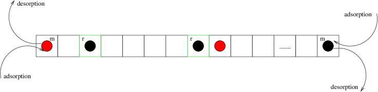
Figure 1: Picture of a Single-File System with two types of adsorbates, $\rm A$(lighter colored) and $\rm B$(darker colored). The marginal sites are labeled with $m$, and the reactive sites(lighter colored) with $r$. Adsoption of $\rm A$ and desorption of $\rm A$ and $\rm B$ can take place only at the two marginal sites. An $\rm A$ can transform into a $\rm B$ only on $r$ labeled sites.

We consider two types of adsorbates, $\rm A$ and $\rm B$, in our model and we denote with $\rm X$ the site occupation of a site, $\rm X$=($\rm*$, $\rm A$, $\rm B$), which stands for an empty site, a site occupied by $\rm A$, or a site occupied by a $\rm B$, respectively. The sites at the ends of the system are labeled with $m$, and the reactive sites are labeled with $r$ (see figure 1). We restrict ourselves to the following mono and bi-molecular transitions.

a) Adsorption and desorption

Adsorption and desorption take place only at the two marginal sites i.e., the left and rightmost sites at the ends of the system.

${\rm A}({\rm gas})$ + $\rm*_{\it m}$ $\longrightarrow$ ${\rm A}_{\it m}$

${\rm A}_{\it m}$ $\longrightarrow$ ${\rm A}({\rm gas})$ + ${\rm*}_{\it m}$

${\rm B}_{\it m}$ $\longrightarrow$ ${\rm B}({\rm gas})$ + $*_{\it m},$

where $\it m$ denotes a marginal site. Note that there is no $\rm B$ adsorption. $\rm B$’s are formed only by a reaction.

b) Diffusion

In the pipe, particles are allowed to diffuse via hopping to vacant nearest neighbor sites.

${\rm A}_{\it n}$ + ${\rm*}_{\it n+1}$ $\longleftrightarrow$ ${\rm*}_{\it n}$ + ${\rm A}_{\it n+1}$

${\rm B}_{\it n}$ + ${\rm*}_{\it n+1}$ $\longleftrightarrow$ ${\rm*}_{\it n}$ + ${\rm B}_{\it n+1},$

where the subscripts are site indices: $n$=1, 2, …, S-1.

c) Reaction

An $\rm A$ can transform into a $\rm B$ at a reactive site.

$\rm A_{\it r}$ $\longrightarrow$ $\rm B_{\it r}$.

The initial state of the system is all that all sites are empty (no particles in the pipe). In this paper we will only look at steady-state properties and not to the time dependence of the system properties starting with no particles.

II.2 Master Equation

Reaction kinetics is described by a stochastic process. Every reaction has a microscopic rate constant associated with it that is the probability per unit time that the reaction occurs. Stochastic models of physical systems can be modelled by a Master Equation. Kampen (1981)

By $\alpha$, $\beta$, we will indicate a particular configuration of the system i.e., a particular way to distribute adsorbates over all the sites. $P_{\alpha}(t)$ will indicate the probability of finding the system in configuration $\alpha$ at time $t$ and $W_{\alpha\beta}$ is the rate constant of the reaction changing configuration $\beta$ to configuration $\alpha$.

The probability of the system being in configuration $\alpha$ at time $t+dt$ can be expressed as the sum of two terms. The first term is the probability to find the system already in configuration $\alpha$ at time $t$ multiplied by the probability to stay in this configuration during $dt$. The second term is the probability to find the system in some other configuration $\beta$ at time $t$ multiplied by the probability to go from $\beta$ to $\alpha$ during $dt$.

$$P_{\alpha}(t+dt)=(1-dt\sum_{\beta}W_{\beta\alpha})P_{\alpha}(t)+dt\sum_{\beta}W_{\alpha\beta}P_{\beta}(t)$$ (1)

By taking the limit $dt\to 0$ this equation reduces to a Master Equation:

$${dP_{\alpha}(t)\over dt}=\sum_{\beta}\left[W_{\alpha\beta}P_{\beta}(t)-W_{\beta\alpha}P_{\alpha}(t)\right].$$ (2)

Analytical results can be derived as follow. The value of a property $X$ is a weighted average over the values $X_{\alpha}$ which is the value of $X$ in configuration $\alpha$:

$$\langle X\rangle=\sum_{\alpha}P_{\alpha}X_{\alpha}.$$ (3)

From this follows the rate equation

$$\begin{split}{{d\langle X\rangle}\over{dt}}&=\sum_{\alpha}{dP_{\alpha}\over{dt}}X_{\alpha}\cr&=\sum_{\alpha\beta}[W_{\alpha\beta}P_{\beta}-W_{\beta\alpha}P_{\alpha}]X_{\alpha}\cr&=\sum_{\alpha\beta}W_{\alpha\beta}P_{\beta}(X_{\alpha}-X_{\beta}).\end{split}$$ (4)

II.3 Dynamic Monte Carlo

Because it might be not always possible to solve the Master Equation analytically, DMC methods allow us to simulate the system governed by the Master Equation over time. We simplify the notation of the Master Equation by defining a matrix $\bf W$ containing the rate constants $W_{\alpha\beta}$, and a diagonal matrix $\bf R$ by ${R}_{{\alpha}{\beta}}\equiv\sum_{\gamma}W_{\gamma\beta}$, if ${\alpha}={\beta}$, and 0 otherwise. If we put the probabilities of the configurations $P_{\alpha}$ in a vector $\bf P$, we can write the Master Equation as

$${d{\bf P}\over{dt}}=-({\bf R}-{\bf W}){\bf P}.$$ (5)

where $\bf R$ and $\bf W$ are assumed to be time independent. We also introduce a new matrix $\bf Q$, ${\bf Q}(t)\equiv\exp[-{\bf R}t].$

This matrix is time dependent by definition and we can rewrite the Master Equation in the integral form

$${\bf P}(t)={\bf Q}(t){\bf P}(0)+\int_{0}^{t}dt^{\prime}{\bf Q}(t-t^{\prime}){\bf W}{\bf P}(t^{\prime}).$$ (6)

By substitution we get of the right-hand-side for $P(t^{\prime})$

$$\begin{split}{\bf P}(t)&=[{\bf Q}(t)\cr&+\int_{0}^{t}dt^{\prime}{\bf Q}(t-t^{\prime}){\bf W}{\bf Q}(t^{\prime})\cr&+\int_{0}^{t}dt^{\prime}\int_{0}^{t^{\prime}}dt^{\prime\prime}{\bf Q}(t-t^{\prime}){\bf W}{\bf Q}(t^{\prime}-t^{\prime\prime}){\bf W}{\bf Q}(t^{\prime\prime})\cr&+\ldots]{\bf P}(0).\end{split}$$ (7)

Suppose at $t=0$ the system is in configuration $\alpha$ with probability $P_{\alpha}(0)$. The probability that, at time $t$, the system is still in configuration $\alpha$ is given by $Q_{\alpha\alpha}(t)P_{\alpha}(0)=\exp(-R_{\alpha\alpha}t)P_{\alpha}(0)$. This shows that the first term represents the contribution to the probabilities when no reaction takes place up to time $t$. The matrix $\bf W$ determines how the probabilities change when a reaction takes place. The second term represents the contribution to the probabilities when no reaction takes place between times $0$ and $t^{\prime}$, some reaction takes place at time $t^{\prime}$, and then no reaction takes place between $t^{\prime}$ and $t$. The subsequent terms represent contributions when two, three, four, etc. reactions take place. The idea of the DMC method is not to compute probabilities $P_{\alpha}(t)$ explicitly, but to start with some particular configuration, representative for the initial state of the experiment one wants to simulate, and then generate a sequence of other configurations with the correct probability. The method generates a time $t^{\prime}$ when the first reaction occurs according to the probability distribution $1-\exp[-R_{\alpha\alpha}t]$. At time $t^{\prime}$ a reaction takes place such that a new configuration ${\alpha}^{\prime}$ is generated by picking it out of all possible new configurations $\beta$ with a probability proportional to $W_{{\alpha}^{\prime}{\alpha}}$. At this point we can proceed by repeating the previous steps, drawing again a time for a new reaction and a new configuration.

III Results and Discussion

III.1 No conversion

We mention in this section various results for the system without conversion. These results can be derived analytically. The derivations are not difficult, so for completeness we give them in the appendix. We will use the results when we deal with the system with conversion.

In a Single-File System without conversion, the relevant processes to describe are adsorption, desorption and diffusion. So, $W_{\alpha\beta}$ is given by

$$W_{\alpha\beta}=W_{\rm ads}\Delta_{\alpha\beta}^{({\rm ads})}+W_{\rm des}\Delta_{\alpha\beta}^{({\rm des})}+W_{\rm diff}\Delta_{\alpha\beta}^{({\rm diff})},$$ (8)

where $\Delta_{\alpha\beta}^{({\rm rx})}$ equals 1 if a reaction of type “rx” can transform the system from $\beta$ to $\alpha$, and equals 0 otherwise. $W_{\rm ads}$, $W_{\rm des}$, $W_{\rm diff}$ are the rate constants of adsorption, desorption and diffusion respectively.

If we substitute expression (8) into the Master Equation (2), we get

$${dP_{\alpha}\over dt} =W_{\rm ads}\sum_{\beta}\left[\Delta_{\alpha\beta}^{({\rm ads})}P_{\beta}-\Delta_{\beta\alpha}^{({\rm ads})}P_{\alpha}\right]$$

$$+W_{\rm des}\sum_{\beta}\left[\Delta_{\alpha\beta}^{({\rm des})}P_{\beta}-\Delta_{\beta\alpha}^{({\rm des})}P_{\alpha}\right]$$ (9)

$$+W_{\rm diff}\sum_{\beta}\left[\Delta_{\alpha\beta}^{({\rm diff})}P_{\beta}-\Delta_{\beta\alpha}^{({\rm diff})}P_{\alpha}\right].$$

Using this expression we can show that when the system is in steady state then the probability of finding the system in a certain configuration depends only on the number of particles in the system.

$$P_{\alpha}=q\big{(}N_{\alpha}\big{)}$$ (10)

where $N_{\alpha}$ is the number of particles in configuration $\alpha$.

The expression for $q(N)$ is:

$$q(N)=\left[{W_{\rm des}\over W_{\rm des}+W_{\rm ads}}\right]^{S}\left[{W_{\rm ads}\over W_{\rm des}}\right]^{N}.$$ (11)

Note that diffusion has here no effect on steady-state properties.

The loading of the pipe, defined as the average number of particles per site, is then

$${Q_{\rm A}={1\over{S}}{{\sum_{N=0}^{S}N\,p(N)}}}={W_{\rm ads}\over W_{\rm ads}+W_{\rm des}},$$ (12)

where $p(N)$ is the probability that there are $N$ particles in the system. Note again that diffusion doesn’t influence the steady-state loading.

The standard deviation, i.e., the fluctuation in the number of particles is then:

$$\begin{split}\sqrt{{\sigma}^{2}}&=\sqrt{\sum_{N=0}^{S}N^{2}\,p(N)-\left[\sum_{N=0}^{S}N\,p(N)\right]^{2}}\cr&=\sqrt{{W_{\rm ads}W_{\rm des}\over(W_{\rm des}+W_{\rm ads})^{2}}S}.\end{split}$$ (13)

To determine how the parameters of the system influence the kinetics of the system, we are interested in the correlation in the occupancy between neighboring sites. We look at one site occupancy and at two sites occupancies. We denote by $\langle{\rm A}_{n}\rangle$ the probability that an $\rm A$ is at site $n$ and with $\langle{\rm A}_{n}{\rm A}_{n+1}\rangle$ the probability to have an $\rm A$ at site $n$ and one at site $n+1$.

One and two-site probabilities can be derived from the fact that all configurations with the same number of particles have equal probability and the expressions for $q(N)$. We find

$${\langle{\rm A}_{n}\rangle}={W_{\rm ads}\over{W_{\rm ads}+W_{\rm des}}},$$ (14)

and

$$\langle{\rm A}_{n}{\rm A}_{n+1}\rangle={\left[{W_{\rm ads}\over{W_{\rm ads}+W_{\rm des}}}\right]}^{2},$$ (15)

Note that this probability does not depend on the site, all sites have equal probability to be occupied and that there is no correlation between the occupation of neighboring sites. Again diffusion doesn’t influence these properties. Note also that these expressions are the same as for a model in which particles are allowed to pass each other.

III.2 All sites reactive

We look first at the situation with all sites reactive: i.e., conversion of an $\rm A$ into a $\rm B$ particle can take place at any site including the marginal sites. For simplicity we consider $W_{\rm desA}$=$W_{\rm desB}$=$W_{\rm des}$, and also $W_{\rm diffA}$=$W_{\rm diffB}$=$W_{\rm diff}$. We will be looking at the total loading ($Q$), the total loading of $\rm A$’s ($Q_{\rm A}$), the total loading of $\rm B$’s ($Q_{\rm B}$), the number of $\rm B$’s produced per unit time (${B}_{prod}$), and how the distribution of $\rm A$’s and $\rm B$’s varies from site to site ($\langle{\rm A}_{n}\rangle$ and $\langle{\rm B}_{n}\rangle$).

Note that the total loading of the pipe for the model with conversion is the same as for the model without conversion

$$Q={W_{\rm ads}\over{W_{\rm ads}+W_{\rm des}}}.$$ (16)

The loadings and the production of $\rm B$’s can easily be derived from the probabilities $\langle{\rm A}_{n}\rangle$ and $\langle{\rm B}_{n}\rangle$ so we first focus on them. For a non-marginal site we can write

$${d\langle{\rm A}_{n}\rangle\over{dt}}={R_{n}}^{({\rm A,diff})}+R_{n}^{(\rm rx)},$$ (17)

where ${R_{n}}^{\rm(A,diff)}$ is the rate of diffusion of $\rm A$ from and to site $n$, and ${R_{n}}^{\rm(rx)}$ is the rate of conversion of $\rm A$ to $\rm B$ on site $n$. The conversion takes place at one site and is therefore easier to handle than the diffusion. Using equation (4) we have

$${R_{n}}^{\rm(rx)}=W_{\rm rx}\sum_{\alpha\beta}{{\Delta}_{\alpha\beta}}^{\rm(rx)}P_{\beta}({\rm A}_{n\alpha}-{\rm A}_{n\beta}),$$ (18)

where ${\rm A}_{n\alpha}=1$ if site $n$ is occupied by an $\rm A$ in configuration $\alpha$ and ${\rm A}_{n\alpha}=0$ if not. We have ${\rm A}_{n\alpha}-{\rm A}_{n\beta}\not=0$ if there is an $\rm A$ at site $n$ in configuration $\beta$ (${\rm A}_{n\beta}$=1) that has reacted to a $\rm B$ leading to configuration $\alpha$ (${{\rm A}_{n\alpha}=0}$). This gives us

$${R_{n}}^{\rm(rx)}=-W_{\rm rx}{{\sum_{\beta}}^{\prime}P_{\beta}}=-W_{\rm rx}\langle{\rm A}_{n}\rangle,$$ (19)

where the prime restricts the summation to those $\beta$’s with ${\rm A}_{n\beta}=1$. For the diffusion we similarly get

$${R_{n}}^{(\rm A,diff)}=W_{\rm diff}\sum_{\beta}{{\Delta}_{\alpha\beta}}^{(\rm A,diff)}P_{\beta}({\rm A}_{n\alpha}-{\rm A}_{n\beta}).$$ (20)

There are four ways in which ${\rm A}_{n\alpha}-{\rm A}_{n\beta}\not=0$ and ${\Delta_{\alpha\beta}}^{\rm(A,diff)}\not=0$ in $\beta$: there is an $\rm A$ at site $n$ that can move to site $(n-1)$, there is an $\rm A$ at site $n$ that can move to $(n+1)$, there is an $\rm A$ at site $(n-1)$ that can move to site $n$ and there is an $\rm A$ at site $(n+1)$ that can move to site $n$. In all cases we have ${{\Delta}_{\alpha\beta}}^{\rm(A,diff)}=1.$ In the first two cases we have ${\rm A}_{n\alpha}-{\rm A}_{n\beta}=-1$ and in the last two we have ${\rm A}_{n\alpha}-{\rm A}_{n\beta}=1.$ The summation over $\beta$ in the first case is restricted to configurations with an $\rm A$ at site $n$ and a vacant site $(n-1)$. This gives a term $-W_{\rm diff}\langle*_{n-1}{\rm A}_{n}\rangle.$ The other cases give terms $-W_{\rm diff}\langle{\rm A}_{n}*_{n+1}\rangle$, $W_{\rm diff}\langle{\rm A}_{n-1}*_{n}\rangle$, and $W_{\rm diff}\langle*_{n}{\rm A}_{n+1}\rangle.$ The rate equations then becomes

$$\begin{split}{d\langle{\rm A}_{n}\rangle\over{dt}}&=W_{\rm diff}[-\langle{\rm A}_{n}*_{n-1}\rangle-\langle*_{n-1}{\rm A}_{n}\rangle+\langle{\rm A}_{n-1}*_{n}\rangle\cr&+\langle*_{n}{\rm A}_{n+1}\rangle]-W_{\rm rx}\langle{\rm A}_{n}\rangle.\end{split}$$ (21)

For $\langle{\rm B}_{n}\rangle$ we get similarly

$$\begin{split}{d\langle{\rm B}_{n}\rangle\over{dt}}&=W_{\rm diff}[-\langle{\rm B}_{n}*_{n-1}\rangle-\langle*_{n-1}{\rm B}_{n}\rangle+\langle{\rm B}_{n-1}*_{n}\rangle\cr&+\langle*_{n}{\rm B}_{n+1}\rangle]+W_{\rm rx}\langle{\rm A}_{n}\rangle.\end{split}$$ (22)

The marginal sites have also adsorption and desorption. They can be dealt with as the conversion. The rate equations for $\rm A$ are

$$\begin{split}{d\langle{\rm A}_{1}\rangle\over{dt}}&=W_{\rm diff}[-\langle{\rm A}_{1}*_{2}\rangle+\langle*_{1}{\rm A}_{2}\rangle]+W_{\rm ads}\langle*_{1}\rangle\cr&-W_{\rm des}\langle{\rm A}_{1}\rangle-W_{\rm rx}\langle{\rm A}_{1}\rangle,\cr{d\langle{\rm A}_{S}\rangle\over{dt}}&=W_{\rm diff}[-\langle{\rm A}_{S}*_{S-1}\rangle+\langle*_{S}{\rm A}_{S-1}\rangle]+W_{\rm ads}\langle*_{S}\rangle\cr&-W_{\rm des}\langle{\rm A}_{S}\rangle-W_{\rm rx}\langle{\rm A}_{S}\rangle,\cr\end{split}$$ (23)

and the rate equations for $\rm B$

$$\begin{split}{d\langle{\rm B}_{1}\rangle\over{dt}}&=W_{\rm diff}[-\langle{\rm B}_{1}*_{2}\rangle+\langle*_{1}{\rm B}_{2}\rangle]-W_{\rm des}\langle{\rm B}_{1}\rangle+W_{\rm rx}\langle{\rm A}_{1}\rangle,\cr{d\langle{\rm B}_{S}\rangle\over{dt}}&=W_{\rm diff}[-\langle{\rm A}_{S}*_{S-1}\rangle+\langle*_{S}{\rm A}_{S-1}\rangle]-W_{\rm des}\langle{\rm B}_{1}\rangle\cr&+W_{\rm rx}\langle{\rm A}_{S}\rangle.\end{split}$$ (24)

Note that these coupled sets of differential equations are exact.

III.2.1 Mean Field results

We will now look at the loadings $Q_{\rm A}$ and $Q_{\rm B}$ and the site occupation probabilities $\langle{\rm A}_{n}\rangle$ and $\langle{\rm B}_{n}\rangle$. We will first determine steady-state properties using the (MF) approximation: i.e, we put $\langle{\rm A}_{n}*_{n+1}\rangle$=$\langle{\rm A}_{n}\rangle\langle*_{n+1}\rangle$ etc. in the rate equations. This gives us

$$\begin{split}0&={W_{\rm diff}W_{\rm des}\over W_{\rm ads}+W_{\rm des}}\left[\big{\langle}{{\rm A}_{n+1}}\big{\rangle}+\big{\langle}{{\rm A}_{n-1}}\big{\rangle}-2\big{\langle}{{\rm A}_{n}}\big{\rangle}\right]-W_{\rm rx}\big{\langle}{{\rm A}_{n}}\big{\rangle},\cr 0&={W_{\rm diff}W_{\rm des}\over W_{\rm ads}+W_{\rm des}}\left[\big{\langle}{{\rm B}_{n+1}}\big{\rangle}+\big{\langle}{{\rm B}_{n-1}}\big{\rangle}-2\big{\langle}{{\rm B}_{n}}\big{\rangle}\right]+W_{\rm rx}\big{\langle}{{\rm A}_{n}}\big{\rangle},\cr 0&={W_{\rm diff}W_{\rm des}\over W_{\rm ads}+W_{\rm des}}\left[\big{\langle}{{\rm A}_{2}}\big{\rangle}-\big{\langle}{{\rm A}_{1}}\big{\rangle}\right]-W_{\rm rx}\big{\langle}{{\rm A}_{1}}\big{\rangle}-W_{\rm des}\big{\langle}{{\rm A}_{1}}\big{\rangle}\cr&+{W_{\rm ads}W_{\rm des}\over W_{\rm ads}+W_{\rm des}},\cr 0&={W_{\rm diff}W_{\rm des}\over W_{\rm ads}+W_{\rm des}}\left[\big{\langle}{{\rm B}_{2}}\big{\rangle}-\big{\langle}{{\rm B}_{1}}\big{\rangle}\right]+W_{\rm rx}\big{\langle}{{\rm A}_{1}}\big{\rangle}-W_{\rm des}\big{\langle}{{\rm B}_{1}}\big{\rangle},\cr 0&={W_{\rm diff}W_{\rm des}\over W_{\rm ads}+W_{\rm des}}\left[\big{\langle}{{\rm A}_{S-1}}\big{\rangle}-\big{\langle}{{\rm A}_{S}}\big{\rangle}\right]-W_{\rm rx}\big{\langle}{{\rm A}_{S}}\big{\rangle}-W_{\rm des}\big{\langle}{{\rm A}_{S}}\big{\rangle}\cr&+{W_{\rm ads}W_{\rm des}\over W_{\rm ads}+W_{\rm des}},\cr 0&={W_{\rm diff}W_{\rm des}\over W_{\rm ads}+W_{\rm des}}\left[\big{\langle}{{\rm B}_{S-1}}\big{\rangle}-\big{\langle}{{\rm B}_{S}}\big{\rangle}\right]+W_{\rm rx}\big{\langle}{{\rm A}_{S}}\big{\rangle}-W_{\rm des}\big{\langle}{{\rm B}_{S}}\big{\rangle}.\cr\end{split}$$ (25)

We have used here the probability for a site to be vacant that we have determined for the case without conversion.

We note that these equations are identical to the MF equations of a system in which the particles can move independently with a rate constant for diffusion equal to ${W_{\rm diff}W_{\rm des}}/{(W_{\rm des}+W_{\rm ads})}$. This means that the MF does not really model the non-passing that characterizes a Single-File System.

The continuum limit of the MF equation is

$$\begin{pmatrix}{\partial a}/{\partial t}\cr{\partial b}/{\partial t}\cr\end{pmatrix}=D\begin{pmatrix}1-b&a\cr b&1-a\cr\end{pmatrix}\begin{pmatrix}{\partial^{2}a}/\partial x^{2}\cr{\partial^{2}b}/\partial x^{2}\cr\end{pmatrix}+W_{\rm rx}\begin{pmatrix}-a\cr a\cr\end{pmatrix},$$ (26)

where $a$=$a(x,t)$ is the probability distribution of $\rm A$’s (a similar definition holds for $b$), and $D$=${{W}_{\rm diff}}d^{2}$, with $d$ the distance between neighboring sites(see appendix). These are the equations that are normally used to describe diffusion in Single-File Systems. Coppens et al. (1998); Krishna et al. (1999); Paschek and Krishna (2001, 2000) As this equation is derived from the MF equations, it has the same drawback; i.e., the Single-File behavior is only incorporated by the reduction of the diffusion, but it does effectively allow for passing of particles. This shows up as so-called counter diffusion of A’s and B’s. Krishna et al. (1999); Paschek and Krishna (2001, 2000)

We see that equations (25) are linear and we can solve them at least numerically. We think however that it is worthwhile to use an analytical approach. We consider the ansatz

$$\big{\langle}{{\rm A}_{n}}\big{\rangle}\propto x^{n}$$ (27)

in the steady-state equations (25) for $\langle{\rm A}_{n}\rangle.$ This leads to

$$x^{2}-2(1+\alpha)x+1=0,$$ (28)

with

$$\alpha={{W_{\rm rx}\over 2W_{\rm diff}}{W_{\rm des}+W_{\rm ads}\over{W_{\rm des}}}}.$$ (29)

The quadratic equation yields two solutions $x_{1}$ and $x_{2}$ with ${x_{2}}={x_{1}^{-1}}.$ We have $x_{1}=x_{2}=1$ only when $\alpha=0$, i.e. when $W_{\rm rx}=0.$ We will therefore assume $\alpha>0$ and $x_{1}<1.$ Then

$$x_{1}=(1+\alpha)-\sqrt{\alpha(\alpha+2)}.$$ (30)

We can write then the solution $\langle{\rm A}_{n}\rangle=a_{1}(x_{1})^{n}+a_{2}(x_{1})^{S+1-n}$. The symmetry in the occupancy of the pipe $\langle{\rm A}_{n}\rangle=\langle{\rm A}_{S+1-n}\rangle$ yields $a_{1}=a_{2}=a$. So, the general solution for the steady state has the form:

$$\big{\langle}{{\rm A}_{n}}\big{\rangle}=a(x_{1}^{n}+x_{1}^{S+1-n}).$$ (31)

The coefficient $a$ is to be determined from the equations for the marginal sites in the set of equations(25). In the left side of the system $n$ is small and $(S+1-n)$ is large. Because $x_{1}<1$ we can neglect the second term in equation (21) and $\big{\langle}{{\rm A}_{n}}\big{\rangle}\propto{x_{1}}^{n}.$ This means that the probability of finding an $\rm A$ at site in the left-hand-side of the system is an exponentially decreasing function of the site index. If we write $\langle{\rm A}_{n}\rangle\propto e^{-{n\over{\Delta}}}$, we find $\Delta=-{1/{ln(x_{1})}}$ for the characteristic length of the decrease. The logarithm makes this length only a slowly varying function of the rate constants(see figure  2). When $W_{\rm diff}$ becomes larger, $\alpha$ approaches 0, $x_{1}$ approaches 1 and $\Delta$ diverges. Note that this is a MF result. We will see that in the simulations $\Delta$ remains finite. Also when the conversion is slow more $\rm A$’s are found away from the marginal sites. The second factor in the expression for $\alpha$ equals the reciprocal of a site being vacant. Low loading leads to a smaller $\alpha$ than high loading. Because of the vacancies the $\rm A$’s can penetrate farther into the system before being converted. For slow conversion or fast diffusion $\alpha$ is small and $\Delta$ can be approximated by

$$\Delta=\sqrt{{W_{\rm diff}\over{W_{\rm rx}}}{W_{\rm des}\over{W_{\rm des}+W_{\rm ads}}}}.$$ (32)

Figure 2: The characteristic length $\Delta$ as a function of $x_{1}$.

Figure 3: ${B}_{prod}$ per unit time at one marginal site as a function of $W_{\rm ads}$ for $S$=${N_{reac}}$=30, $W_{\rm des}$=0.8, $W_{\rm diff}=2$ and $W_{\rm rx}=0.4$.

The total loading with $\rm A$’s, $Q_{\rm A}$, is

$$Q_{\rm A}={1\over{S}}\sum_{n=1}^{S}\langle{\rm A}_{n}\rangle$$ (33)

so, the expression for $Q_{\rm A}$ is

$$Q_{\rm A}={a\over{S}}\sum_{n=1}^{S}[{x_{1}}^{n}+{x_{1}}^{S+1-n}]={{2a}\over{S}}{{x_{1}{(1-{x_{1}}^{S})}}\over{1-x_{1}}},$$ (34)

$$Q_{\rm B}=Q-Q_{\rm A}.$$ (35)

The total production of $\rm B$’s is

$${B}_{prod}=W_{\rm rx}Q_{\rm A}S=2aW_{\rm rx}{{x_{1}({1-{x_{1}}^{S}})}\over{1-x_{1}}}.$$ (36)

III.2.2 Simulation results

We present now the results for different sets of parameters and we compare them with MF results. Because we can see from equation (36) that larger pipes don’t increase the productivity of the system, we consider for the comparisons of the results a system size $\textsl{S}=30$. We have considered separately the sets of parameters in Table 1.

set	$W_{\rm ads}$	$W_{\rm des}$	$W_{\rm diff}$	$W_{\rm rx}$
a)	0.2	0.8	0.05	0.01
b)	0.2	0.8	0.05	0.1
c)	0.2	0.8	2	0.1
d)	0.2	0.8	1	2
e)	0.2	0.8	10	2
f)	0.8	0.2	0.05	0.01
g)	0.8	0.2	0.05	0.1
h)	0.8	0.2	2	0.1
i)	0.8	0.2	1	2
j)	0.8	0.2	10	2

Table 1: The sets of parameters used for the simulations

The sets of parameters from a) to e) are for the cases of low loading and from f) to j) for the high loading. The parameters in the table describe the following situations: a) and f) for very slow reaction and slow diffusion; b) and g) for slow reaction and slow diffusion; c) and h) for slow reaction and fast diffusion; d) and i) for fast reaction and slow diffusion; e) and j) for fast reaction and fast diffusion.

	$Q_{\rm A}$		${B}_{prod}$		Q
set	MF	Sim	MF	Sim	Sim
a)	0.0330	0.0318	0.0099	0.0100	0.209
b)	0.0149	0.0148	0.0491	0.0472	0.198
c)	0.0385	0.0342	0.1156	0.1024	0.204
d)	0.0040	0.0041	0.2449	0.2463	0.200
e)	0.0046	0.0044	0.2767	0.2729	0.201
f)	0.0798	0.0748	0.0239	0.0235	0.795
g)	0.0376	0.0373	0.1129	0.1157	0.804
h)	0.0598	0.0486	0.1796	0.1406	0.802
i)	0.0048	0.0049	0.2931	0.2943	0.797
j)	0.0050	0.0049	0.3013	0.2957	0.801

Table 2: Simulation and MF results for $Q_{\rm A}$ and ${B}_{prod}$ for all the sets of parameters

We can see from Table 2 that the simulation and MF results match for all the cases except the cases when we have low reaction rates and fast diffusion for both low and high loading. In these cases MF overestimates the amount of $\rm A$’s in the pipe, and consequently overestimates the B production. In figure 4 we have the site occupancy with $\rm A$ and $\rm B$ both from the simulations and MF. We again see that the MF and the simulation results agree reasonably well, except for low reaction rates and fast diffusion. MF overestimates the characteristic length $\Delta$ and allows $\rm A$’s to penetrate farther into the pipe than in the simulations. The reason for this is that MF describes the fact that the particles cannot pass each other by reducing the diffusion, but this effectively does allow for passing. The larger $\Delta$ in MF means also a larger $Q_{\rm A}$. As a consequence the $\rm B$ production in MF is larger and, because these $\rm B$’s have to be able to leave the pipe via desorption, the probabilities $\langle{\rm B}_{1}\rangle$ and $\langle{\rm B}_{S}\rangle$ are larger in MF. The probabilities $\langle{\rm A}_{1}\rangle$ and $\langle{\rm A}_{S}\rangle$ are therefore smaller, which means that the MF curves and the simulation curves in figure cross each other, as can actually be seen. The behavior of the system at high loading and at low loading is about the same, except that $\Delta$ is smaller at high loading.

Figure 4: The site occupancy with $\rm A$ ($\langle{\rm A}_{n}\rangle$) and $\rm B$ ($\langle{\rm B}_{n}\rangle$) as a function on site number for cases a, b, c, d, e when $S=N_{reac}=30$. The continuous line and the corresponding symmetric line represent MF results for $\langle{\rm A}_{n}\rangle$ and $\langle{\rm B}_{n}\rangle$ respectively. The dashed lines represent DMC results for $\langle{\rm A}_{n}\rangle$ and $\langle{\rm B}_{n}\rangle$. $\langle{\rm A}_{n}\rangle$ is decreasing towards the middle of the pipe while $\langle{\rm B}_{n}\rangle$ is increasing.

One might expect that the larger the number of reactive sites the more $\rm B$’s will be produced in the pipe. From the simulations we see that the amount of $\rm B$’s produced per unit time by all reactive sites goes to a limit value when the number of reactive sites is increased. In figure 5, the marked line represents the $\rm B$ production as a function on the length of the pipe and the dashed line the $\rm B$ production according to MF. For short pipe lengths, the $\rm B$ production from both MF and simulations increase linearly with S, while for higher lengths it converges to a limiting value. The limiting value is higher for MF. This could be seen also from the Table 2. According to MF there are more $\rm B$ produced in the pipe.

Figure 5: $\rm B$ production as a function on the length of the pipe for $W_{\rm ads}$=0.2, $W_{\rm des}$=0.8, $W_{\rm diff}$=2, and $W_{\rm rx}$=0.1. The marked line represents the DMC results and the dashed line represents the MF results.

For the case $W_{\rm ads}\to\infty$ we have

$${B}_{prod}={{2W_{\rm rx}W_{\rm des}}\over{W_{\rm rx}+W_{\rm des}}}.$$ (37)

From the simulations (see figure 3) we see that for high adsorption rates, ${B}_{prod}$ converges to a point and the corresponding value is equal to the analytical value for the case adsorption is infinitely fast. The reason for this is that all the sites are occupied, diffusion is completely suppressed, and only the marginal sites play a role. The expression above can be seen as a factor 2 for the two marginal sites, the probability that an $\rm A$ at the marginal sites is converted to a $\rm B$ before it desorbs $W_{\rm rx}/{W_{\rm rx}+W_{\rm des}}$, and the rate constant for desorption $W_{\rm des}$.

The accuracy of the simulation results for $Q_{\rm A}$ and $B_{prod}$ can be derived by looking at the total loading $Q$ in Table 2. For the total loading $Q$, the simulation results can be compared with the values of the exact expression (12). We remark that the largest deviation from the exact analytical results is 0.04, so the relative errors are around 0.02$\%$.

The differences between MF and the simulations becomes especially clear in the limit $W_{\rm diff}\to\infty$. Because this limit makes the system homogeneous in MF we get

$$Q_{\rm B}={W_{\rm ads}\over{W_{\rm ads}+W_{\rm des}}}{W_{\rm rx}\over{W_{\rm rx}+W_{\rm des}}},$$ (38)

$$Q_{\rm A}={W_{\rm ads}\over{W_{\rm ads}+W_{\rm des}}}{W_{\rm des}\over{W_{\rm rx}+W_{\rm des}}}.$$ (39)

The first factor in these expressions is the probability that a site is occupied. The second factor indicates if the particle is converted to a $\rm B$ or not before it desorbs. The simulations show that the system should not be homogeneous at all (see figure 6). The $\rm B$ production increases linearly with $S$ only for the case of infinitely-fast diffusion, otherwise it converges to a limiting value.

Figure 6: Analytical and simulation results for site occupancy of a system when parameters are: $S=N_{reac}=30$, $W_{\rm ads}$=0.8, $W_{\rm des}$=0.2, $W_{\rm diff}$=100 and $W_{\rm rx}$=2. The continuous line and the corresponding symmetric line represent the simulation profiles for site occupancy with $A$ and $B$ particles. The bottom and the upper straight lines represent the analytical results for occupancy with $\rm{A}$ and with $\rm{B}$ particles respectively.

III.3 Only some of the sites reactive

We consider now the situation that not all the sites are reactive, and that these reactive sites can be either uniformly distributed inside the pipe or distributed in compact blocks. We will show that the number of reactive sites doesn’t change qualitatively the properties of the system. $Q_{\rm A}$, $Q_{\rm B}$ and number of $\rm B$ produced for a variable number of reactive sites are compared with the previous results.

III.3.1 Mean Field

From the Master Equation it is easy to show that the total loading is again just the same as in the case when all the sites are reactive. We introduce an extra coefficient $\Delta_{n}$ in the MF equations to the reaction term. $\Delta_{n}=1$ if $n$ is a reactive site and $\Delta_{n}=0$ if it is not a reactive site. The steady-state equations are identical to equations (25), except that $W_{\rm rx}$ should be replaced by $W_{\rm rx}\Delta_{n}$. The resulting set of equations is linear again and it should be possible to solve them numerically. In fact only the probabilities for the marginal and reactive sites have to be solved numerically. For the other sites the probabilities can be obtained by simple linear interpolation. That this is correct can be seen because those sites only have the diffusion term. We can also remove the probabilities for the $\rm B$’s, because we have from the model without conversion that

$$\big{\langle}{{\rm A}_{n}}\big{\rangle}+\big{\langle}{{\rm B}_{n}}\big{\rangle}=1-\big{\langle}{*_{n}}\big{\rangle}={W_{\rm ads}\over W_{\rm ads}+W_{\rm des}}.$$ (40)

The resulting equations for the reactive sites have the same form as equation (25) for the non-marginal sites. We expect therefore that we get an exponential decrease of $\langle{\rm A}_{n}\rangle$ on the reactive sites when we move from the marginal sites to the center of the pipe, and a linear dependence on $n$ between the unreactive sites.

III.3.2 Simulation results

The number of reactive sites is considered to vary from 1 to 50$\%$ and the reactive sites are distributed either in blocks situated near the marginal sites, in the middle of the pipe, or homogeneously distributed in the pipe. We will first compare the MF results with the MC simulation results for different sets of parameters and then we look at the dependence of $\rm B$ production and total loading $Q_{\rm A}$ on the number and position of reactive sites. For the comparison between MF and MC results we consider the system size $\textsl{S}=30$ and the number of reactive sites $N_{reac}=10$. The sets of parameters used for the specific situations to be studied are the same as the sets used in the case with all the sites reactive in the previous section.

	Marginal		Middle		Homogeneous
set	MF	Sim	MF	Sim	MF	Sim
a)	0.0512	0.0500	0.0731	0.0771	0.0208	0.0469
b)	0.0153	0.0152	0.0712	0.0788	0.0138	0.0206
c)	0.0590	0.0672	0.0901	0.0881	0.0719	0.0594
d)	0.0041	0.0041	0.0667	0.0730	0.0120	0.0123
e)	0.0067	0.0006	0.0447	0.0583	0.0126	0.0121
f)	0.0896	0.0752	0.3008	0.3473	0.1121	0.1056
g)	0.0376	0.0369	0.2850	0.3383	0.0585	0.0605
h)	0.0871	0.0579	0.2844	0.3250	0.1227	0.0867
i)	0.0048	0.0048	0.2606	0.3137	0.0319	0.0413
j)	0.0056	0.0053	0.1556	0.2826	0.0175	0.0289

Table 3: Simulation and MF results for $Q_{\rm A}$ for all the sets of parameters in the cases of homogeneous distribution of the reactive sites, blocks of reactive sites in the middle of the pipe and near the marginal sites ($S=30$, $N_{reac}=10$)

	Marginal		Middle		Homogeneous
set	MF	Sim	MF	Sim	MF	Sim
a)	0.0099	0.0099	0.0001	0.0000	0.0011	0.0045
b)	0.0449	0.0477	0.0001	0.0008	0.0153	0.0117
c)	0.1156	0.1021	0.0393	0.0216	0.0728	0.0521
d)	0.2449	0.2492	0.0283	0.0161	0.1357	0.0891
e)	0.2767	0.2763	0.1482	0.0646	0.2410	0.1899
f)	0.0239	0.0235	0.0014	0.0006	0.0086	0.0076
g)	0.1129	0.1160	0.0015	0.0000	0.0139	0.1171
h)	0.1796	0.1421	0.0470	0.0059	0.1212	0.0661
i)	0.2931	0.2941	0.0288	0.0069	0.1526	0.0897
j)	0.3013	0.2965	0.1552	0.0143	0.2713	0.1739

Table 4: Simulation and MF results for ${B}_{prod}$ for all the sets of parameters in the cases of homogeneous distribution of the reactive sites, blocks of reactive sites in the middle of the pipe and near the marginal sites ($S=30$, $N_{reac}=10$)

We can see from the Tables 3 and  4 that when the reactive sites are homogeneously distributed or situated as a block in the middle of the pipe, there are significant differences between MF results and MC results. When the reactive sites form blocks near the marginal sites, the results are almost the same as when all sites are reactive: the MC and the MF results differ if we have fast diffusion and slow reaction. The sites in the center of the pipe are not relevant when the sites at the ends of the pipe are reactive. When the reactive sites are situated only in the middle of the pipe, we have deviations for all the sets of parameters. They are very prominent for the case when we have high loading, fast diffusion and fast reaction. MF strongly underestimates $\rm A$’s for all non-reactive sites, but we have also important deviations for high loading in the cases with fast diffusion-slow reaction, slow diffusion-fast reaction, and slow diffusion-slow reaction. This is happening because for high loading, the end sites will always be occupied by a particle $\rm A$ and the $\rm B$’s will not be able to get out of the pipe. In MF particles effectively can pass each other, so $\rm B$ particles are then able to get out of the pipe. Even for the case of low loading we still have deviations from MF for fast diffusion and fast reaction. In this case MF overestimates $\rm A$’s for nonreactive sites. For fast diffusion and slow reaction, MF underestimates $\rm A$’s for nonreactive sites and for slow diffusion and slow reaction MF overestimates $\rm B$’s for the reactive sites in the middle.

Figure 7: The site occupancy for the cases a, b, c, d, e -homogeneous distribution. The continuous line and the corresponding symmetric line represent the MF results. The other dashed lines represent the DMC results.

Figure 8: The site occupancy for the cases f, g, h, i, j - middle sites reactive, $N_{reac}=10$. The continuous line and the corresponding symmetric line represent the MF results. The other dashed lines represent the DMC results.

Figures  7 and  8 show how the probabilities $\langle{{\rm A}_{n}}\rangle$ and $\langle{{\rm B}_{n}}\rangle$ vary in the pipe. The situations for reactive sites forming blocks at the ends of the pipe are not shown as they are almost the same as when all the sites are reactive (see figure 4). When the reactive sites are homogeneously distributed the plots look also very similar to the ones with all sites reactive, except that the characteristic length $\Delta$ is larger. $\langle{{\rm A}_{n}}\rangle$ and $\langle{{\rm B}_{n}}\rangle$ look very different when the reactive sites form a block in the middle of the pipe. The MF results show, as predicted, a linear behavior at the nonreactive sites. The MC results show, however, a nonlinear behavior in the form of S-like curves. At the reactive sites the behavior is similar to the situation with all sites reactive with the MC results showing a more rapid approach to the value at the middle of the pipe than MF, i.e., smaller $\Delta$. The values at the marginal sites can differ between MC and MF quite a lot. This reflects the difference in ${B}_{prod}$ mentioned before: a different ${B}_{prod}$ must be accompanied by a different $\rm B$ desorption at steady-state. As we have already seen from the case when all the sites were reactive, ${B}_{prod}$ very rapidly approaches the limiting value when the pipe is made longer (see figure 5). Similarly when we start with few reactive sites and, instead of increasing the length of the pipe, we increase the number of reactive sites. The loading $Q_{\rm B}$ is already almost the same as the value with all sites reactive when only about 10$\%$ of all sites are reactive provided there are reactive sites at or very near the marginal sites. If the reactive sites are moved away from the ends of the pipe, then the loading $Q_{\rm B}$ and the $\rm B$ production decreases.

IV Summary

We have used analytical and simulation techniques to study the reactivity in Single-File Systems.

The MF results show that MF models Single-File behavior by changing the diffusion rate constant, but it effectively does allow passing of particles.

When all the sites are reactive, the simulation and MF results are very similar for all the parameters, except for the case when we have low reaction rates and fast diffusion. In these cases MF overestimates the amount of $\rm A$’s in the pipe. The amount of $\rm B$ produced per unit time by all reactive sites goes to a limit value when the number of reactive sites is increased. For high adsorption rates, ${B}_{prod}$ converges to a point and the corresponding value is equal to the analytical value for the case adsorption is infinitely fast. The sites in the middle of the pipe have no effect on the $B$ production. The differences between MF and the simulations becomes especially clear in the limit ${W_{\rm diff}}\to\infty$.

When only some of the sites are reactive, there are significant differences between MF and MC results when the reactive sites are homogeneously distributed or situated as a block in the middle of the pipe. When the reactive sites form blocks near the marginal sites, the results are almost the same as when all sites are reactive: The MC and the MF results differ only when we have fast diffusion and slow reaction. The sites in the center of the pipe are not relevant when the sites at the ends of the pipe are reactive. When the reactive sites are situated in the middle of the pipe, we have deviations for all the sets of parameters. They are very prominent for the case when we have high loading, fast diffusion and fast reaction. MF strongly underestimates $\rm A$’s for all non-reactive sites, but we have also important deviations for high loading in the cases with fast diffusion-slow reaction, slow diffusion-fast reaction, slow diffusion-slow reaction. The MF results show a linear behavior at the nonreactive sites. The MC results show, however, a nonlinear behavior in the form of S-like curves. The loading $Q_{\rm B}$ is already almost the same as the value with all sites reactive when only about 10$\%$ of all sites are reactive provided there are reactive sites at or very near the marginal sites. If the reactive sites are moved away from the ends of the pipe, then the loading $Q_{\rm B}$ and the $\rm B$ production decreases.

V Acknowledgments

The authors thank Prof.dr. R.A. van Santen for many stimulating discussions.

VI Appendix

VI.1 Probability to find the system in a certain configuration. Loadings and fluctuations.

We show the existence of a function $q$, depending only on the number of particles such that

$$P_{\alpha}=q\big{(}n(\alpha)\big{)}$$ (41)

is the steady-state solution of the Master Equation (2) for a system without conversion, where $n(\alpha)$ is the number of particles in configuration $\alpha$. The second part of the proof consists of showing the uniqueness of the solution.

Substitution of $P_{\alpha}=q\big{(}n(\alpha)\big{)}$ in equation (9) shows that the last term in the Master Equation vanishes, because $\Delta_{\alpha\beta}^{({\rm diff})}=\Delta_{\beta\alpha}^{({\rm diff})}$ and $n(\alpha)=n(\beta)$. The other terms can also be simplified by using how the number of particles changes upon adsorption and desorption.

$${dP_{\alpha}\over dt} =W_{\rm ads}\left[q\big{(}n(\alpha)-1\big{)}\sum_{\beta}\Delta_{\alpha\beta}^{({\rm ads})}-q\big{(}n(\alpha)\big{)}\sum_{\beta}\Delta_{\beta\alpha}^{({\rm ads})}\right]$$

$$+W_{\rm des}\left[q\big{(}n(\alpha)+1\big{)}\sum_{\beta}\Delta_{\alpha\beta}^{({\rm des})}-q\big{(}n(\alpha)\big{)}\sum_{\beta}\Delta_{\beta\alpha}^{({\rm des})}\right].$$ (42)

A further simplification is possible if we realize that desorption reverses the effect of an adsorption and vice versa. This means $\Delta_{\alpha\beta}^{({\rm des})}=\Delta_{\beta\alpha}^{({\rm ads})}$. This leads to

$${dP_{\alpha}\over dt} =\left[q\big{(}n(\alpha)-1\big{)}W_{\rm ads}-q\big{(}n(\alpha)\big{)}W_{\rm des}\right]\sum_{\beta}\Delta_{\alpha\beta}^{({\rm ads})}$$

$$-\left[q\big{(}n(\alpha)\big{)}W_{\rm ads}-q\big{(}n(\alpha)+1\big{)}W_{\rm des}\right]\sum_{\beta}\Delta_{\beta\alpha}^{({\rm ads})}.$$ (43)

We denote by $N$, the number of particles in a certain configuration, $N=n(\alpha)$. We see that we get a steady-state solution for

$${dP_{\alpha}\over dt}=0,$$ (44)

provided by

$${q(N+1)\over q(N)}={W_{\rm ads}\over W_{\rm des}}$$ (45)

for $N={\textsl{0, 1, 2,\ldots, S-1}}$. (Note that the case $N=S$ in the Master Equation presents no problems, because the summation over $\beta$ yields zero.)

The second step consists of showing that this solution is the only one. This part for instance can be found in Chapter 5 of Van Kampen. Kampen (1981)

VI.2 Derivation of function q(N)

Expression (45) leads to

$$q(N)=C\left[{W_{\rm ads}\over W_{\rm des}}\right]^{N},$$ (46)

where $C$ is some normalization constant. We can compute it from

$$1 =\sum_{\alpha}P_{\alpha}=\sum_{\alpha}q\big{(}n(\alpha)\big{)}=\sum_{N=0}^{S}\left({S\atop N}\right)q(N)$$

$$=C\sum_{N=0}^{S}\left({S\atop N}\right)\left[{W_{\rm ads}\over W_{\rm des}}\right]^{N}=C\left[{W_{\rm des}+W_{\rm ads}\over W_{\rm des}}\right]^{S}.$$ (47)

The combinatorial factor after the third equal sign derives from the number of configurations with $N$ particles. The last step uses

$$(x+y)^{S}=\sum_{N=0}^{S}\left({N\atop n}\right)x^{N-n}y^{n}.$$ (48)

The expression for $q(N)$ now becomes

$$q(N)=\left[{W_{\rm des}\over W_{\rm des}+W_{\rm ads}}\right]^{S}\left[{W_{\rm ads}\over W_{\rm des}}\right]^{N}.$$ (49)

Note that this expression does not depend on $W_{\rm diff}$: i.e., diffusion has no effect at all on steady-state properties.

The probability $p(N)$ that there are $N$ particles in the system is given by

$$p(N)=\begin{pmatrix}S\cr N\cr\end{pmatrix}q(N)=\left({S\atop N}\right)\left[{W_{\rm des}\over W_{\rm des}+W_{\rm ads}}\right]^{S}\left[{W_{\rm ads}\over W_{\rm des}}\right]^{N}.$$ (50)

This follows from (49). With this formula we can compute all statistical properties of the number of particles. The average number of particles is

$$\sum_{N=0}^{S}N\,p(N) =\left[{W_{\rm des}\over W_{\rm des}+W_{\rm ads}}\right]^{S}\sum_{N=0}^{S}\left({S\atop N}\right)N\left[{W_{\rm ads}\over W_{\rm des}}\right]^{N}$$ (51)

$$={W_{\rm ads}\over W_{\rm des}+W_{\rm ads}}S.$$ (52)

The loading of the pipe, defined as the average number of particles per site, is

$${Q_{\rm A}={{\sum_{N=0}^{S}N\,p(N)}\over S}}={W_{\rm ads}\over W_{\rm ads}+W_{\rm des}}.$$ (53)

The average squared number of particles is

$$\sum_{N=0}^{S}N^{2}\,p(N) =\left[{W_{\rm des}\over W_{\rm des}+W_{\rm ads}}\right]^{S}\sum_{N=0}^{S}\left({S\atop N}\right)N^{2}\left[{W_{\rm ads}\over W_{\rm des}}\right]^{N}$$ (54)

$$={W_{\rm ads}(W_{\rm des}+SW_{\rm ads})\over(W_{\rm des}+W_{\rm ads})^{2}}S.$$ (55)

The variance, i.e., the square of the fluctuation in the number of particles, is then

$$\sum_{N=0}^{S}N^{2}\,p(N)-\left[\sum_{N=0}^{S}N\,p(N)\right]^{2}={W_{\rm ads}W_{\rm des}\over(W_{\rm des}+W_{\rm ads})^{2}}S.$$ (56)

VI.3 Derivation of the one-site and two-sites occupancy for the model without conversion

The probability that site $n$ is occupied by $\rm A$ is given by

$$\begin{split}{\langle{\rm A}_{n}\rangle}&=\sum_{\alpha}P_{\alpha}{\Delta}_{\alpha}^{(n)},\cr&=\sum_{N}\sum_{\alpha\in N}P_{\alpha}{\Delta}_{\alpha}^{(n)},\cr&=\sum_{N}q(N)\sum_{\alpha\in N}{\Delta}_{\alpha}^{(n)},\cr&=\sum_{N=1}^{S}q(N)\left({{S-1}\atop{N-1}}\right),\cr&={\left[W_{\rm des}\over{W_{\rm des}+W_{\rm ads}}\right]}^{S}\sum_{N=1}^{S}\left({{S-1}\atop{N-1}}\right){\left[{W_{\rm ads}}\over{W_{\rm des}}\right]}^{N},\cr&={\left[W_{\rm des}\over{W_{\rm des}+W_{\rm ads}}\right]}^{S}{W_{\rm ads}\over{W_{\rm des}}}{\left[1+{W_{\rm ads}\over{W_{\rm des}}}\right]}^{S-1},\cr&={W_{\rm ads}\over{W_{\rm ads}+W_{\rm des}}},\cr\end{split}$$ (57)

where ${\Delta}_{\alpha}^{(n)}$ is 1 if site $n$ in configuration $\alpha$ is occupied by an $\rm A$ particle, and it is 0 otherwise. The combinatorial factor denotes the number of ways the particles except the one at site $n$ can be distributed over the remaining sites. Knowing the one-site occupancy we can derive the two-site occupancy

$$\begin{split}{\langle{\rm A}_{n}{\rm A}_{n+1}\rangle}&=\sum_{\alpha}P_{\alpha}\Delta_{\alpha}^{(n)}\Delta_{\alpha}^{(n+1)},\cr&=\sum_{N}\sum_{\alpha\in N}P_{\alpha}\Delta_{\alpha}^{(n)}\Delta_{\alpha}^{(n+1)},\cr&=\sum_{N}q(N)\sum_{\alpha\in N}\Delta_{\alpha}^{(n)}\Delta_{\alpha}^{(n+1)},\cr&=\sum_{N=2}^{S}q(N)\left({{S-2}\atop{N-2}}\right),\cr&={\left[W_{\rm des}\over{W_{\rm des}+W_{\rm ads}}\right]}^{S}\sum_{N=2}^{S}\left({{S-2}\atop{N-2}}\right){\left[{W_{\rm ads}}\over{W_{\rm des}}\right]}^{N},\cr&={\left[W_{\rm des}\over{W_{\rm des}+W_{\rm ads}}\right]}^{S}{\left({W_{\rm ads}\over{W_{\rm des}}}\right)}^{2}{\left[1+{W_{\rm ads}\over{W_{\rm des}}}\right]}^{S-2},\cr&={\left({W_{\rm ads}\over{W_{\rm ads}+W_{\rm des}}}\right)}^{2}.\cr\end{split}$$ (58)

VI.4 Continuum limit

The rate equation for the A’s is

$$\begin{split}{d\langle{\rm A}_{n}\rangle}\over{dt}&={W}_{\rm diff}[{\langle{\rm A}_{n-1}*_{n}\rangle}+{\langle*_{n}{\rm A}_{n+1}\rangle}-{\langle{\rm A}_{n}*_{n+1}\rangle}\cr&-{\langle*_{n-1}{\rm A}_{n}\rangle}]-W_{\rm rx}{\langle{\rm A}_{n}\rangle}.\cr\end{split}$$ (59)

The MF approximation of this equation is

$$\begin{split}{d\langle{\rm A}_{n}\rangle}\over{dt}&={W}_{\rm diff}[({\langle{\rm A}_{n-1}\rangle}+{\langle{\rm A}_{n+1}\rangle}){\langle*_{n}\rangle}\cr&-{\langle{\rm A}_{n}\rangle}(\langle*_{n-1}\rangle+\langle*_{n+1}\rangle)]\cr&-W_{\rm rx}{\langle{\rm A}_{n}\rangle}.\cr\end{split}$$ (60)

If we take the continuum limit and denote by $a=a(x,t)$, $b=b(x,t)$ and $v=v(x,t)$ the probability distribution of $\rm A$’s, $\rm B$’s and vacancies respectively, and if we use Taylor series for the diffusion term, the equation becomes

$$\begin{split}{{\partial a}\over{\partial t}}&={W}_{\rm diff}[a((n-1)d,t)+a((n+1)d,t)]v(nd,t)\cr&-{W}_{\rm diff}a(nd,t)[v((n-1)d,t)+v((n+1)d,t)]a(nd,t)-W_{\rm rx}a\cr&\approx{W}_{\rm diff}\left[a-d{{\partial a}\over{\partial x}}+{1\over{2}}d^{2}{{\partial^{2}a}\over{\partial x^{2}}}+a+d{{\partial a}\over{\partial x}}+{1\over{2}}{{\partial^{2}a}\over{\partial x^{2}}}\right]v\cr&-{W}_{\rm diff}\left[v-d{{\partial v}\over{\partial x}}+{1\over{2}}d^{2}{{\partial^{2}v}\over{\partial x^{2}}}+v+d{{\partial v}\over{\partial x}}+{1\over{2}}{{\partial^{2}v}\over{\partial x^{2}}}\right]a-W_{\rm rx}a\cr&={W}_{\rm diff}\left[2a+d^{2}{{\partial^{2}a}\over{\partial x^{2}}}\right]v-{W}_{\rm diff}a\left[2v+d^{2}{{\partial^{2}v}\over{\partial x^{2}}}\right]-W_{\rm rx}a\cr&={W}_{\rm diff}d^{2}\left[v{{\partial^{2}a}\over{\partial x^{2}}}+a{{\partial^{2}a}\over{\partial x^{2}}}+a{{\partial^{2}b}\over{\partial x^{2}}}\right]-W_{\rm rx}a\cr&={W}_{\rm diff}d^{2}\left[(1-b){{\partial^{2}a}\over{\partial x^{2}}}+a{{\partial^{2}b}\over{\partial x^{2}}}\right]-W_{\rm rx}a,\cr\end{split}$$ (61)

where $d$ is the distance between sites. A similar relation can be derived for $b(x,t)$. With $D\equiv{W_{\rm diff}}d^{2}$ we can write

$$\begin{pmatrix}{\partial a}/{\partial t}\cr{\partial b}/{\partial t}\cr\end{pmatrix}=D\begin{pmatrix}1-b&a\cr b&1-a\cr\end{pmatrix}\begin{pmatrix}{\partial^{2}a}/\partial x^{2}\cr{\partial^{2}b}/\partial x^{2}\cr\end{pmatrix}+W_{\rm rx}\begin{pmatrix}-a\cr a\cr\end{pmatrix}.$$ (62)

VI.5 MF derivation of the total loading $Q_{A}$ in case with conversion

The total loading with $\rm A$’s, $Q_{\rm A}$, is written as

$$Q_{\rm A}={1\over{S}}\sum_{n=1}^{S}\langle{\rm A}_{n}\rangle,$$ (63)

so, the expression for $Q_{\rm A}$ is

$$\begin{split}Q_{\rm A}&={a\over{S}}\sum_{n=1}^{S}[{x_{1}}^{n}+{x_{1}}^{S+1-n}],\cr&={a\over{S}}\sum_{n=1}^{S}{x_{1}}^{n}+{a\over{S}}\sum_{n=1}^{S}{x_{1}}^{S+1-n},\cr&={{2a}\over{S}}\sum_{n=1}^{S}{x_{1}}^{n},\cr&={{2a}\over{S}}{{x_{1}{(1-{x_{1}}^{S})}}\over{1-x_{1}}}.\end{split}$$ (64)

References

- Abrams and Corbin (1995) L. Abrams and D. R. Corbin, J. of Inclusion Phenomena and Molecular Recognition in Chemistry 21, 1 (1995).
- Meier et al. (1996) W. H. Meier, D. H. Olson, and C. Baerlocher, Atlas of Zeolite Structure Types (Elsevier, London, 1996).
- Sholl and Fichthorn (1997) D. S. Sholl and K. A. Fichthorn, Physical Review E 55(6), 7753 (1997).
- Keffer et al. (1996a) D. Keffer, A. V. McCormick, and H.T.Davis, Mol. Phys. 87, 367 (1996a).
- Keffer et al. (June 1995) D. Keffer, A. V. McCormick, and H.T.Davis, in Proceedings from the XI International Workshop on Condensated Matter Theories, Caracas (June 1995).
- Keffer et al. (1996b) D. Keffer, A. V. McCormick, and H.T.Davis, J. Phys. Chem. 100, 967 (1996b).
- Keffer et al. (1996c) D. Keffer, A. V. McCormick, and H.T.Davis, J. Phys. Chem. 100, 638 (1996c).
- J.G.Tsikoyannis and Wei (1991) J.G.Tsikoyannis and J. Wei, Chem. Eng. Sci. 46, 233 (1991).
- Rdenbeck et al. (1997) C. Rdenbeck, J. Krger, and K.Hahn, Physical Review E 55, 5697 (1997).
- Okino et al. (1999) M. S. Okino, R. Q. Snurr, H. H. Kung, J. E. Ochs, and M. L. Mavrovouniotis, J. Chem. Phys. 111, 2210 (1999).
- Krger et al. (1992) J. Krger, M. Petzold, H.Pfeifer, S.Ernst, and J.Weitkamp, J. Catal. 136, 283 (1992).
- van Beijeren et al. (1983) H. van Beijeren, K. W. Kehr, and R. Kutner, Phys. Rev. B 28, 5711 (1983).
- Rdenbeck et al. (1995) C. Rdenbeck, J. Krger, and K.Hahn, J. Catal. 157, 656 (1995).
- Nelson and Auerbach (1999) P. H. Nelson and S. M. Auerbach, J. Chem. Phys. 18, 110 (1999).
- Auerbach and Metiu (1996) S. M. Auerbach and H. I. Metiu, J. Chem. Phys. 106, 2893 (1996).
- Saravanan and Auerbach (1999) C. Saravanan and S. M. Auerbach, J. Chem. Phys. 110(22), 11000 (1999).
- Saravanan and Auerbach (1997) C. Saravanan and S. M. Auerbach, J. Chem. Phys. 107(19), 8132 (1997).
- Coppens et al. (1999a) M.-O. Coppens, A. Bell, and Chakraborty, Chem. Engng. Sci. 54, 3455 (1999a).
- Coppens et al. (1998) M.-O. Coppens, A. Bell, and Chakraborty, Chem. Engng. Sci. 53, 2053 (1998).
- Coppens et al. (1999b) M.-O. Coppens, A. Bell, and Chakraborty, Scientific Computing in Chemical Engineering pp. 200–207 (1999b).
- Kampen (1981) V. Kampen, Stochastic Processes in Physics and Chemistry (Elsevier Science Publishers B.V., 1981).
- Krishna et al. (1999) R. Krishna, T. J. H. Vlugt, and B. Smit, Chem. Eng. Sci. 54, 1751 (1999).
- Paschek and Krishna (2001) D. Paschek and R. Krishna, Physical Chemistry Chemical Physics 3, 3185 (2001).
- Paschek and Krishna (2000) D. Paschek and R. Krishna, Physical Chemistry Chemical Physics 2, 2389 (2000).
- R.J.Gelten et al. (1998a) R.J.Gelten, R. Santen, and A.P.J.Jansen, Israel J.Chem. 38, 415 (1998a).
- R.J.Gelten et al. (1998b) R.J.Gelten, A.P.J.Jansen, R. Santen, J.J.Lukkien, and P. Hilbers, J.Chem.Phys. 108(14), 5921 (1998b).
- Lukkien et al. (1998) J. Lukkien, J. Segers, P.A.J.Hilbers, R.J.Gelten, and A.P.J.Jansen, Phys.Rev.E 58, 2598 (1998).
- Keil et al. (2000) F. J. Keil, R. Krishna, and M.-O. Coppens, Rev. Chem. Engng 16, 71 (2000).