Nonresonant corrections to the 1s-2s two-photon resonance
for the hydrogen atom.

Abstract

The nonresonant (NR) corrections are estimated for the most accurately measured two-photon transition 1s-2s in the hydrogen atom. These corrections depend on the measurement process and set a limit for the accuracy of atomic frequency measurements. With the measurement process adopted in the modern experiments the NR contribution for 1s-2s transition energy can reach $10^{-3}$ Hz while the experimental inaccuracy is quoted to be $\pm$ 46 Hz.

PACS numbers: 31.30.Jv, 12.20.Ds, 0620Jr., 31.15.-p

Nonresonant (NR) corrections have been first introduced in Ref. [1] where the modern QED theory of the natural line profile in atomic physics has been formulated. The NR corrections indicate the limit up to which the concept of the energy of an excited atomic state has a physical meaning - that is the resonance approximation. In the resonance approximation the line profile is described by the two parameters: energy $E$ and width $\Gamma$ . Beyond this approximation the specific role of $E$ and $\Gamma$ should be replaced by the complete evaluation of the line profile for the particular process. If the distortion of the Lorentz profile is small one can still consider the NR correction as an additional energy shift. Unlike all other energy corrections, this correction depends on the particular process which has been employed for the measurement of the energy difference. Quite independent of the accuracy of theoretical calculations of the ”traditional” energy corrections which can be much poorer than the experimental accuracy, NR corrections define the principal limit for the latter. One can state that nonresonant corrections set the limit for the accuracy of all the atomic frequency standards.

Nonresonant corrections have been evaluated for H-like ions of phosphorus (Z=15) and uranium (Z=92) in Refs. [2, 3]. While for uranium the NR correction turned out to be negligible, its value was comparable with the experimental error bars in case of phosphorus. Recently the NR correction has been evaluated for the Lyman-$\alpha$ 1s-2p transition in hydrogen [4]. In [4] the process of the resonance photon scattering was considered as a standard procedure for the determination of the energy levels. According to [1] the parametric estimate of the NR correction to the total cross-section is (in relativistic units):

$$\delta_{1}=c_{1}m\alpha^{2}(\alpha Z)^{6}$$ (1)

Here $\alpha$ denotes the fine structure constant, $m$ is the electron mass, $Z$ is the nuclear charge number and $c_{1}$ abbreviates a numerical factor. Evaluations in [4] yielded $c_{1}=-1.31*10^{-3}$ and $\delta_{1}=-1.30$ Hz. In Ref. [4] a factor $4/9$ was missing in the expression for $c_{1}$. Moreover, there exists another NR correction to the total cross section of the same process, connected with the contribution of the near-resonant $2p_{3/2}$ state (see below):

$$\delta_{2}=c_{2}m\alpha^{4}(\alpha Z)^{4}$$ (2)

For the hydrogen atom ($Z=1$) this correction is parametrically of the same order, but numerically it is larger than (1): $c_{2}=4.94\,10^{-3}$, $\delta_{2}=4.89$ Hz. Finally, the ”asymmetry” correction, which is of the same order, arises from the resonant term when replacing the width $\Gamma(\omega_{0})$, where $\omega_{0}$ is the resonant frequency, by $\Gamma(\omega)$. In the case of the Lyman-alpha transition $\Gamma(\omega_{0})=\left(\frac{2}{3}\right)^{8}\alpha^{3}$ a.u. should be replaced by $\Gamma(\omega)=(2^{11}/3^{9})\alpha^{3}\omega$ a.u. This result corresponds to the ”velocity” form of the transition amplitude. The ”length” form that follows from the ”velocity” form after the gauge transformation would yield $\Gamma(\omega)=(2^{17}/3^{11})\alpha^{3}\omega^{3}$ a.u. The ”asymmetry” shift is different for the ”velocity” and the ”length” forms. However, we should remember that the ”velocity” form follows originally from the QED description and that the gauge transformation in the simple form mentioned above does exist only at the resonance frequency. The additional ”asymmetry” shift which follows from the ”velocity” form of $\Gamma(\omega)$ is given by $\delta_{3}=c_{3}m\alpha^{2}(\alpha Z)^{6}$ with $c_{3}=\left(\frac{2}{3}\right)^{17}=1.015*10^{-3}$ yielding $\delta_{3}=1.007$ Hz. The $\omega$-dependent terms in the Lorentz denominator lead to smaller NR contributions [1]. Still the accuracy for the Lyman-$\alpha$ frequency measurements is much poorer: about $6$ MHz [5]. Modern experimental techniques employed in Lamb-shift measurements are based on two-photon resonances, in particular for the transition 1s-2s [6, 7]. In the present paper we provide an estimate for the NR correction to the transition frequency in this case.

The magnitude of the NR corrections depends strongly on the conditions of the experiment. It is important whether total or differential cross sections are measured since some NR corrections vanish after the angular integration. In [4] the following expression for the NR correction to the frequency of the one-photon transition, which applies in case when the total cross section scattering is measured, has been derived:

$$\delta_{1}=-\frac{1}{4}\frac{\Gamma_{A^{\prime}}^{2}}{\Gamma_{A^{\prime}A}\Gamma_{BA^{\prime}}}Re\left[\sum_{n\neq A^{\prime}}\frac{\Gamma_{AA;A^{\prime}n}\Gamma_{BB;nA^{\prime}}}{E_{n}-E_{A^{\prime}}}+\sum_{n^{\prime}}\frac{\Gamma_{An;A^{\prime}B}\Gamma_{nB;AA^{\prime}}}{E_{n}+E_{A^{\prime}}-E_{A}-E_{B}}\right]\quad.$$ (3)

Here $B$, $n$, and $A$ denote initial, intermediate and final electron states, respectively. $A^{\prime}$ lables the resonant intermediate state. Then $\Gamma_{A^{\prime}}$ is the total width and $\Gamma_{A^{\prime}A}$, $\Gamma_{BA^{\prime}}$ are partial widths, connected with the transitions $A^{\prime}\rightarrow A$ and $B\rightarrow A^{\prime}$. The notations $\Gamma_{AB;CD}$ are used for the ”mixed” transition probabilities where one amplitude corresponds to the transition $A\rightarrow C$ and the other one to the transition $B\rightarrow D$. Finally, $E_{B}$, $E_{A^{\prime}}$ and $E_{n}$ denote the one-electron energies. In case of the Lyman-$\alpha$ transition $B=A=1s,A^{\prime}=2p$ and the photon frequency is close to $\omega=E_{2p}-E_{1s}$. Then $\Gamma_{A^{\prime}}=\Gamma_{A^{\prime}A}=\Gamma_{BA^{\prime}}=\Gamma_{2p}$. Assuming that the ”mixed” probabilities are parametrically of the same order as $\Gamma_{2p}\simeq m\alpha(\alpha Z)^{4}$ (in relativistic units) and using the parametric estimate $\Delta E\simeq m(\alpha Z)^{2}$ for the energy denominators in Eq. (3) we obtain immediately the estimate (1). An explicit summation over the total energy spectrum for the hydrogen atom leads to the coefficient $c_{1}$ quoted above.

Expression (3) corresponds to the interference term between resonant and nonresonant contributions to the photon scattering amplitude. The nonresonant contributions arise when we replace the resonant intermediate state $2p$ by $np$ states with $n>2$ and also when the incident and emitted photons are interchanged.

In [8] it has been observed that a large NR contribution arises when taking into account the fine structure of the H atom and considering the state $2p_{3/2}$ as a nonresonant one. Then the enhancement follows from the small energy denominator $\Delta E_{f}=E_{2p_{3/2}}-E_{2p_{1/2}}$. However, this contribution vanishes in the total cross section after angular integration and remains only finite if the differential cross section is considered. The latter may correspond to a particular experimental situation but it is the total cross section which defines the absolute limit for the accuracy of the frequency measurement. Additionally, we would like to note that there exists also a quadratic NR contribution to the total cross section from $2p_{3/2}$ state. This contribution does not vanish after angular integration and is given by the formula:

$$\delta_{2}=\frac{(\frac{1}{2}\Gamma_{2p})^{4}}{\Delta E_{f}^{3}}\quad.$$ (4)

This can be easily obtained in the same way as Eq. (3) (see [4]). The parametric estimate Eq. (2) immediately follows from Eq. (4) and from the estimate $\Delta E_{f}=m(\alpha Z)^{4}$.

Formula (3) is valid also for the NR correction to the process of the resonant two-photon excitation $1s+2\gamma\rightarrow 2s$. In this case $B=A=1s,A^{\prime}=2s$, $2\omega=E_{2s}-E_{1s}$, $\Gamma_{A^{\prime}}\simeq\Gamma_{A^{\prime}A}\simeq\Gamma_{B^{\prime}A}=\Gamma_{2s,2\gamma}$. Here $\Gamma_{2s,2\gamma}$ is the two-photon width of the $2s$ level (neglecting the small contribution of the one-photon width $\Gamma_{2s,1\gamma}$). Using the parametric estimate for the two-photon width $\Gamma_{2s,2\gamma}\simeq m\alpha^{2}(\alpha Z)^{6}$ one obtains

$$|\delta|=\frac{\Gamma_{2s,2\gamma}^{2}}{\Delta E}\simeq\frac{[m\alpha^{2}(\alpha Z)^{6}]^{2}}{m(\alpha Z)^{2}}=m\alpha^{4}(\alpha Z)^{10}$$ (5)

This estimate has been derived in Ref. [8] where the conclusion has been drawn, that NR corrections for $1s+2\gamma\rightarrow 2s$ transition enter at the level $10^{-14}$ Hz and thus are negligible at the current and projected level of experimental accuracy. At present the latter is $\pm 46$ Hz and is expected to be two orders of magnitude smaller in future experiments [7].

The NR correction (5) corresponds to the process described by the Feynman graph of Fig. 1. However, the experiment in [6, 7] is based on a different process. In this experiment the H atom being in its ground state is excited first by the absorption of the two laser photons into the $2s$ state. After some time delay $t_{D}$ the $2s$ state is detected by applying a ”small” electric field and observing the quenched Lyman-$\alpha$ decay. The corresponding process is described by the Feynman graph of Fig. 2. For the analysis we will assume that for the ”small” electric field the Stark parameter $\xi_{\rm S}=\langle 2s|\vec{d}\cdot\vec{E}|2p\rangle/\Delta E_{\rm L}$ corresponds to $\xi_{\rm S}\ll 1$. $\vec{d}$ is the electric dipole moment operator, $\vec{E}$ is the electric field strength, $\Delta E_{\rm L}$ is the Lamb shift between $2s$ and $2p$ states. Accordingly, we can replace the intermediate $2s$ state in the graph in Fig. 2 by the state $2s^{\prime}=2s+\xi_{\rm S}2p$. The resonant cross-section corresponding to the Feynman graph of Fig. 2 is determined by

$$\sigma_{{\rm res}}=\frac{1}{2\pi}\,\frac{\Gamma_{2s,2\gamma}\,\xi_{\rm S}^{2}\,\Gamma_{2p,1\gamma}}{(E_{2s}+\Delta E_{s}^{(2)}-E_{1s}-2\omega)^{2}+\frac{1}{4}\xi_{\rm S}^{4}\,\Gamma_{2p,1\gamma}^{2}}\quad.$$ (6)

Here $\Gamma_{2p,1\gamma}$ denotes the Lyman-$\alpha$ width and $\Delta E_{s}^{(2)}$ is the second-order Stark shift for the $2s$ state. The Stark shift for the $1s$ state can be neglected for ”small” electric fields. However, in the real experiment [6, 7] the excitation region is separated spatially from the detection region. Therefore the Stark shift does not contribute to the excitation condition: $2\omega=E_{2s}-E_{1s}$. Moreover, the width of the resonance is defined by the time delay $t_{D}$, which is necessary for the atom to reach the detection region: for $\xi_{\rm S}\sim 0.1$ the decay time in the electric field is $(\xi_{\rm S}^{2}\Gamma_{2p,1\gamma})^{-1}\simeq 10^{-7}$ s. This is very small time compared to $t_{D}$: the characteristic atomic velocities are $10^{4}$ cm/s and the space separation of the excitation and detection regions is $13$ cm [6, 7]. Then $t_{D}\simeq 10^{-3}$ s what corresponds to the experimental width of the resonance $\Gamma_{{\rm exp}}\sim 1$ kHz. Then Eq. (6) should be replaced by

$$\sigma_{{\rm res}}=\frac{1}{2\pi}\,\frac{\Gamma_{2s,2\gamma}\,\Gamma_{{\rm exp}}}{(E_{2s}-E_{1s}-2\omega)^{2}+\frac{1}{4}\Gamma_{{\rm exp}}^{2}}\quad.$$ (7)

The major nonresonant contribution arises from the closely lying $2p$ level

$$\sigma_{{\rm NR}}=\frac{1}{2\pi}\,\frac{\Gamma_{2p,2\gamma}\,\Gamma_{2p,1\gamma}}{(E_{2p}-E_{1s}-2\omega)^{2}+\frac{1}{4}\Gamma_{2p,1\gamma}^{2}}$$ (8)

where $\Gamma_{2p,2\gamma}$ is the two-photon width of the $2p$ level. The interference term between $\sigma_{{\rm res}}$ and $\sigma_{{\rm NR}}$ is absent in the total cross section, but may be present in the differential cross section.

To find the NR correction we employ the same idea as in [4], i.e. we determine the position of the maximum for the function $\sigma(\omega)$.

In the case in which the total cross section is measured we obtain

$$\delta=\frac{\Gamma_{2p,2\gamma}\Gamma_{2p,1\gamma}}{\Gamma_{2s,2\gamma}\Gamma_{{\rm exp}}}\,\frac{(\frac{1}{2}\Gamma_{{\rm exp}})^{4}}{\Delta E_{\rm L}^{3}}$$ (9)

Here we assumed that $\Delta E_{\rm L}\gg\Gamma_{2p,1\gamma}$ where $\Delta E_{\rm L}=E_{2s}-E_{2p}$ is the Lamb shift. The corresponding expressions (in relativistic units) are: $\Gamma_{2p,1\gamma}=\left(\frac{2}{3}\right)^{8}m\alpha(\alpha Z)^{4}=0.04m\alpha(\alpha Z)^{4}$ and $\Delta E_{\rm L}=0.4m\alpha(\alpha Z)^{4}$. Taking into account that $\Gamma_{2p,2\gamma}$ is defined by the E1M1 transition and $\Gamma_{2s,2\gamma}$ corresponds to the 2E1 transition, we have $\Gamma_{2p,2\gamma}/\Gamma_{2s,2\gamma}\simeq(\alpha Z)^{2}$. Insertion of these quantities into Eq. (9) leads to the negligible NR correction. The NR correction to the differential cross-section is much larger. In this case the formula of the type of Eq. (3) for differential cross section should be used:

$$|\delta|=\frac{1}{2}\left(\frac{\Gamma_{2p,2\gamma}\Gamma_{2p,1\gamma}}{\Gamma_{2s,2\gamma}\Gamma_{{\rm exp}}}\right)^{\frac{1}{2}}\frac{(\Gamma_{{\rm exp}})^{2}}{\Delta E_{\rm L}}\simeq 10^{-3}\,{\rm Hz}\quad.$$ (10)

This limit for the experimental accuracy turns out to be many orders of magnitude larger than the corresponding value obtained from (5). It is the value (10) which should be compared with the projected experimental accuracy of about $10^{-1}$ Hz [6, 7].

Acknowledgements

The work of L.L. and D.S. was supported by the RFBR Grant $No.$ 99-02-18526 and by the Minobrazovanie grant $No.$ E00-3.1.-7. G. P. and G. S. acknowledge financial support from BMBF, DFG and GSI.

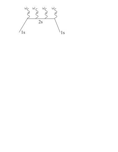
FIG. 1.: The Feynman graph for the resonance excitation of $2s$ level in the double photon scattering process $1s+2\gamma\rightarrow 2s$. The solid line denotes the electrons, the wavy lines with the arrows denote the incident and emitted photons.

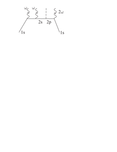
FIG. 2.: The Feynman graph that describes the quenched decay of the intermediate $2s$ state. The electric field is denoted by the dashed line. The other notations are the same as in Fig. 1.

REFERENCES

- [1] F. Low Phys. Rew. 88, 53 (1951)
- [2] L. Labzowsky, V. Karasiev and I. Goidenko, J. Phys. B27, L439 (1994)
- [3] L. N. Labzowsky, I. A. Goidenko and D. Liesen, Phys. Scr. 56, 271 (1997)
- [4] L. N. Labzowsky, D. A. Solovyev, G. Plunien and G. Soff, Phys. Rev. Lett. 87, 143003 (2001)
- [5] K. S. E. Eihema, J. Walz and T. W. Hänsch, Phys. Rev. Lett. 86, 5679 (2001)
- [6] A. Huber, B. Gross,M. Wetz and T. W. Hänsch, Phys. Rev. A59, 1844 (1999)
- [7] M. Niering, R. Holzwarth, J. Reichert, P. Pokasov, Th. Udem, M. Weitz, T. W. Hänsch, P. Lemond, G. Semtarelli, M. Abgrall, P. Lourent, C. Salomon and A. Clairon, Phys. Rev. Lett. 84, 5496 (2000)
- [8] U. D. Jentschura and P. J. Mohr, arXiv: physics/0110053 v.2 25 Oct. 2001