A Novel Method for the Solution of the Schrödinger Eq. in the Presence of Exchange Terms.

Abstract

In the Hartree-Fock approximation the Pauli exclusion principle leads to a Schrödinger Eq. of an integro-differential form. We describe a new spectral noniterative method (S-IEM), previously developed for solving the Lippman-Schwinger integral equation with local potentials, which has now been extended so as to include the exchange nonlocality. We apply it to the restricted case of electron-Hydrogen scattering in which the bound electron remains in the ground state and the incident electron has zero angular momentum, and we compare the acuracy and economy of the new method to three other methods. One is a non-iterative solution (NIEM) of the integral equation as described by Sams and Kouri in 1969. Another is an iterative method introduced by Kim and Udagawa in 1990 for nuclear physics applications, which makes an expansion of the solution into an especially favorable basis obtained by a method of moments. The third one is based on the Singular Value Decomposition of the exchange term followed by iterations over the remainder. The S-IEM method turns out to be more accurate by many orders of magnitude than any of the other three methods described above for the same number of mesh points.

Date text]date Date text]date LABEL:FirstPage1 LABEL:LastPage#1

I
Introduction.

A new very efficient and stable method for solving the Schrödinger equation has recently been developed IEM . This method (S-IEM) solves the Lippman-Schwinger integral equation rather than the differential Schrödinger equation because the numerical errors for the solution of the former are inherently smaller than for the latter, and by making a spectral expansion of the solution into Chebyshev polynomials it acquires additional excellent accuracy properties. This method also avoids the usual drawback of numerical solutions of integral equations, namely, the need to invert large non-sparse matrices which represent the discretized form of the equation. It achieves this by dividing the integration interval into partitions and by making use of the semi-separable nature of the Green’s function in configuration space. The accuracy of the S-IEM has been tested by comparing it to the solution of the differential Schrödinger equation for various cases, such as the scattering of cold atoms IEMA , and for tunneling through a barrier MORSE , but not by comparing it to existing solutions of the integral Lippman-Schwinger equation. The purpose of the present paper is two-fold: a) to extend the S-IEM to the case that there are non-local exchange terms present. This is possible baps , KG without losing the original accuracy and stability features since the kernel of the exchange integral is semi-separable (see below). And b), to compare the accuracy of the extended S-IEM to conventional methods of solving an integral equation in configuration space.

The scattering of an electron from a hydrogen atom offers a good opportunity for performing such a test, because, integral equation methods have been developed in the past in order to include the integral exchange terms required by the Pauli exclusion principle, as is described further below. The present test calculation is physically not realistic since it does not allow for the polarization of the bound electron cloud by the incident electron, or the ionization of the atom. But it is still sufficiently close to realistic so as to serve as an adequate test for the comparison of different algorithms. Realistic calculations which allow for the polarization of the electron cloud involve coupling between many channels BRAY , or else the solution of a two-dimensional differential equation STELBO , which is much beyond the scope of the present work, and is not necessary in order to demonstrate the power of our new method.

The three methods for solving the non-local Schrödinger equation in the presence of the exchange terms we compare our S-IEM with are as follows. One of these methods kouri solves an integral equation which is very similar to the one we solve, with the main difference that it uses a trapezium type method for numerically expressing the integrals, rather than the spectral Chebyshev method used in the S-IEM. Another is an iterative method introduced by Kim and Udagawa in 1990 udagawa  for nuclear physics applications, which makes an expansion of the solution into an especially favorable basis obtained by a method of moments. The third is a variation of a conventional iterative method for including the exchange term. It consists in expanding the exchange kernel into a small number of separable terms by means of the Singular Value Decomposition and then iterating over the remainder essaid . Since there is a rich literature on methods developed for taking the exchange terms into account, a review of some of the methods most relevant to the S-IEM will be described below.

The scattering of electrons from atoms or molecules has been the subject of investigation ever since quantum mechanics was introduced, and the research continues unabated, mainly concerning the scattering of polarized electrons KLEINP or of high energy photons PRATT from atoms or molecules, or charge transfer in ion-molecule scattering SAHA . The latter can also be calculated by using advanced three-body formalisms ALT . One of the features which gives computational difficulties in solving the corresponding Schrödinger equation is the Pauli exclusion principle which requires that the wave function of the incident electron be anti-symmetric with the wave functions of the electrons in the target atom or molecule. In the Hartreee-Fock formulation this requirement leads to the presence of non local terms in the (coupled) differential equations of the form

$$\int_{0}^{\infty}K(r,r^{\prime})\,u(r^{\prime})\,dr^{\prime},$$ (1)

where $u(r)$ is the required solution and $K$ is the integration kernel due to exchange. In the early investigations burke1 the exchange terms were taken into account iteratively, by using Green’s functions defined by the local part of the potential. However, under certain conditions these iterations do not converge burke1 , TEMKIN . Methods to accelerate the convergence have been introduced, but such methods tend to be cumbersome and unpredictable. An improved iteration procedure can be obtained by means of a separable representation of the integral kernelessaid , as is described further below, but this method has its limitations as well. An interesting method to include the exchange terms non-iteratively by approximating them in terms of a separable representations has been developed by Schneider and Collins SCsep . Methods to solve the non-local Schrödinger equation non iteratively and rigorously have also been developed NIEM . One of the oldest ones originated with I. Percival and R. Marriott MARRIOT . It consists in constructing auxiliary functions which are solutions of the differential equation in the presence of several types of inhomogeneous terms and then constructing the exact solution (which take into account the integral exchange terms) by means of linear combinations of the auxiliary functions. A variation of this method was developed by Lamkin and Temkin TEMKIN for their Polarized Orbitals procedure. In this method the semi-separable nature of the exchange kernel $K$

$$K(r,r^{\prime}) =A(r)\,B(r^{\prime})\;\;for\;\;r^{\prime}<r$$

$$K(r,r^{\prime}) =A(r^{\prime})\,B(r)\;\;for\;\;r^{\prime}>r$$ (2)

is exploited. The integral of Eq. (1) then becomes

$$\int_{0}^{\infty}K(r,r^{\prime})\,u(r^{\prime})\,dr^{\prime}=A(r)\,\int_{0}^{r}B(r^{\prime})\,u(r^{\prime})\,dr^{\prime}+B(r)\,\int_{r}^{\infty}A(r^{\prime})\,u(r^{\prime})\,dr^{\prime}$$ (3)

which can be rewritten as

$$\int_{0}^{\infty}K(r,r^{\prime})\,u(r^{\prime})\,dr^{\prime}=A(r)\,\int_{0}^{r}B(r^{\prime})\,u(r^{\prime})\,dr^{\prime}-B(r)\,\int_{0}^{r}A(r^{\prime})\,u(r^{\prime})\,dr^{\prime}+CB(r).$$ (4)

Again auxiliary functions can be obtained by solving the differential integral equation with the constant $C$ set equal to zero or unity. The true solution $u(r)$ is obtained by means of a linear combination of the auxiliary functions, and the constant $C=\int_{0}^{\infty}A(r^{\prime})\,u(r^{\prime})\,dr^{\prime}$ as well as the coefficients of the linear combination can be obtained via the solution of an algebraic equation. The advantage of this method TEMKIN is that, when the integral over the kernel goes from $0$ to $r,$ as is the case in Eq. (4), the solution of the integro-differential equation can be performed easily by starting at the origin and increasing the upper limit gradually from one meshpoint to the next. With a step size of 0.05 the authors obtain accuracies to about three significant figures with this method.

A method which yields five significant figures with the same step size of 0.05 is obtained by Kouri and co-workers kouri . The main difference from Temkin’s method TEMKIN is that the authors first transform the integro-differential equation into a Lippman-Schwinger integral equation, because integral equations have greater numerical stability than differential equations. They again transform the integrals, which originally extend from $0$ to $\infty$ into integrals from $0$ to $r,$ plus inhomogeneous terms, thus obtaining Volterra integral equations of the second kind. They then easily obtain auxiliary solutions to auxiliary Volterra equations by stepping progressively from the origin to increasing values of $r,$ similarly to what is done in the method of Temkin .The exact solution, and the respective constants, can then be determined in a algebraic way similar to what is done in Ref TEMKIN . Smith and Henry NIEM have also developed methods to solve the Volterra type integral equations non iteratively. These methods are generally called NIEM, where the “N” stands for “Non-iterative”. Collins and Schneider also have examined the NIEM form of the non-local Schrödinger equation, CSint but without transforming it into a Volterra type. By discretizing the integral via the trapezoidal rule, they obtain a linear algebraic equation for the wave functions at the mesh points, and for this reason the method is called (LA). The formulation of the initial equation to be solved by our new method is very similar to that of CSint . The main differences, to be discussed below, arise from the numerical techniques used in the solution of these equations (NIEM). For the case of the exchange terms which are due to the Coulomb interaction, as is the case for most atomic physics calsulations, the exchange terms can also be replaced by coupling to a set of ”pseudo-states, a technique which is made use of in the work of Weatherford, Onda and Temkin WOT , and is also illustrated in the present work.

Other methods have been developed to solve the electron-atom scattering equations. One consist in introducing a set of basis functions such as Laguerre polynomials, and expanding both the solution and the target states into this basis exp . Another such expansion basis utilizes sturmian functionssturm . In these procedures the exchange integrals can be carried out, since they contain the known basis wave functions. Finite element representations have also been applied shertz . The R-matrix approach is also well developed R-M  .

As already briefly mentioned above, our new “spectral integral equation method”, S-IEM, transforms the differential equation into an equivalent Lippmann-Schwinger integral equation through the use of Green’s functions, similar to what is done in the older approaches described above. It differs from the older methods in that it uses the Fredholm form of the integral equation (whose range of integration is from $0$ to $r_{\max}$ ), as done in Ref. CSint , and does not transform it into a Volterra type (whose range of integration is from $0$ to the variable radial distance $r$). It thus it avoids the need to evaluate the constants $C$ which occur in theVolterra method, but instead it has to solve for a larger number of other constants. The latter arise by dividing the radial integration interval $[0$ $r_{\max}]$ into partitions, and by expanding the solution in each partition into two independent functions which in turn are obtained by solving a local integral equation through the spectral expansion into Chebyshev Polynomials. There are twice as many such coefficients as there are partitions, and hence the matrix from which the coefficients are calculated is large, say $600\times 600$. However, this matrix is sparse, and hence soluble economically. As is shown here, the semi-separable structure of the exchange nonlocality allows us to preserve the sparseness in the present case as well. If, however, the nonlocal potential is not of the semi-separable form our integral equation method still gives stable and accurate solutions, but then the biggest matrix involved is no longer sparse KKR . From the numerical point of view, the main difference of our S-IEM from other integral equation methods described above is that the radial mesh-points in the S-IEM are not equidistant, while those for the latter are. The numerical errors of the latter are of the finite difference type, and are given by a fixed power of the distance between mesh points, while in the S-IEM the errors become smaller than any power of the distance between mesh points. Or, more precisely, in the S-IEM the errors become smaller than any inverse power of the number of Chebyshev support points in each partition, a property which expresses the spectral nature of the S-IEM. This property permits the S-IEM to have far fewer mesh points than the more conventional discretization formulations of differential or integral equations for a given envisaged accuracy, as will be demonstrated in Fig. 4 below.

The first of our three comparison methods essaid consists in replacing the exchange kernel by a small number of fully separable terms, and carrying out iterations only over the remainder. This is possible because, as is well known, the Green’s function for a Schrödinger equation with both local and non local but fully separable potentials can be obtained without much difficulty by adding terms to the Green’s function distorted only by the local potential. Our second method udagawa is a modified integral equation method, denoted as M-IEM. It uses a set of basis functions which are obtained by applying successively higher powers of the hamiltonian operator with local potentials on an initial scattering wave function. This method has been very successful in applications to nuclear physics problems. The third method IEM , the S-IEM, uses the Lippmann-Schwinger integral form of the Schrödinger equation. It differs from a previously introduced non-iterative solution of the Lippmann-Schwinger integral equation, denoted as NIEM NIEM , in that it uses non-equidistant mesh points, divides the radial interval into partitions of adjustable size, and uses a very accurate spectral integration technique involving Chebyshev polynomials. Because of its inherent stability the S-IEM is likely the method of choice IEMA for situations requiring solutions out to large distances. The generalization of this method so as to include the exchange potential baps , KG is described further below.

In section 2 the basic equation to be solved will be described; in sections 3, 4 and 5 the S-IEM, the SVD-improved iterative method, and the method of moments, respectively, will be reviewed; in section 6 the numerical comparison between the four methods will be described; section 7 contains the summary and conclusion; and Appendix 1 contains further details of the extension of the S-IEM to the presence of exchange.

II Equations and Notations.

The equation describing two electrons, one bound to a hydrogen-like nucleus of charge Z, and another incident with kinetic energy $\overline{E}_{k}$ on the ground state of the atom is

$$-(\hbar^{2}/2\mu)\left[\nabla_{\vec{r}_{1}}^{2}+\nabla_{\vec{r}_{2}}^{2}-\frac{Ze^{2}}{r_{1}}-\frac{Ze^{2}}{r_{2}}+\frac{e^{2}}{r_{12}}\right]\Psi(\vec{r}_{1},\vec{r}_{2})=\overline{E}\;\Psi(\vec{r}_{1},\vec{r}_{2}),\;$$ (5)

where $\Psi(\vec{r}_{1},\vec{r}_{2})$ is the overall wave function, $\overline{E}$ is the total energy, $e$ is the charge of the electron, $\mu$ is the is the reduced mass of the incident electron, $\hbar$ is Planck’s constant, $\vec{r}_{1}$ and $\vec{r}_{2}$ denote the position vectors of the two electrons, $r_{1}$ and $r_{2}$ are the respective magnitudes, and $r_{12}=|\vec{r}_{1}-\vec{r}_{2}|$  is the distance between the two electrons. In order to transform the variables into atomic units, one multiplies Eq.(5) by $(2\mu/\hbar^{2})\,a_{0}^{2}$, where $a_{0}=(\hbar^{2}/\mu e^{2})$ is the Bohr unit of length, with the result

$$\left[-\nabla_{\vec{x}_{1}}^{2}-\nabla_{\vec{x}_{2}}^{2}-\frac{2Z}{x_{1}}-\frac{2Z}{x_{2}}+\frac{2}{x_{12}}\right]\Psi(\vec{r}_{1},\vec{r}_{2})=E\Psi(\vec{r}_{1},\vec{r}_{2}).$$ (6)

Here $\vec{x}=\vec{r}/a_{0}$ is a displacement vector in units of Bohr, and $E=\overline{E}/\Re$ is the total energy in Rydberg units, with $\Re=\hbar^{2}/(2\mu\,a_{0}^{2})$.

In the Hartree-Fock approximation one expands the total wave function in terms of the bound states $\phi_{i},i=1,2,...$ of the atomic electron

$$\Psi(\vec{r}_{1},\vec{r}_{2})=\sum_{i}\left[\psi_{i}(\vec{r}_{1})\;\phi_{i}(\vec{r}_{2})\pm\psi_{i}(\vec{r}_{2})\;\phi_{i}(\vec{r}_{1})\right],\;$$ (7)

where $\psi_{i}$ are the wave functions of the scattered electron in channel $i$ , to be determined from the solution of a set of coupled equations. The $+$ or the $-$ signs occur for the spin singlet or triplet cases, respectively. The subscript $i$ represents the set of all quantum numbers which label the electron bound states. The corresponding principal quantum number is $n_{i}$, and the corresponding bound state energy is $\varepsilon_{i}=-(Z^{2}/n_{i}^{2})\Re$. The case of two or more bound electron states can also be derived. The result is a set of coupled equations with local and non-local pieces in the diagonal and off diagonal potentials. The latter are semi-separable of fully separable, hence the method described here for the one-channel case can also be applied. In the present study only the ground state will be assumed, i.e., $i=1$ , and henceforth this subscript will be dropped, and further, $Z=1$ . Under these assumptions the bound-state electron energy is $\varepsilon=-\Re$ and the incident electron has the asymptotic kinetic energy $\overline{E}_{k}=\overline{E}-\,\varepsilon$ . Assuming that this is a positive quantity, the corresponding wave number $k$ in units of $a_{0}$ is given by

$$k^{2}=E_{k}=\left(\overline{E}-\,\varepsilon_{i}\right)/\Re=E-1.$$ (8)

The equation for $\psi$ is obtained by truncating the sum in Eq. (7) to one term, inserting it into Eq. (6), multiplying on the left by the functions $\phi=\phi_{1}(\overrightarrow{r}_{2})$, and integrating over $d^{3}r_{2}$. In the present numerical study only the case of orbital angular momenta = 0 will be considered. The result is

$$(-\nabla_{x_{1}}^{2}+V(x_{1})-k^{2})\psi(\vec{r}_{1})\pm\left[(-k^{2}+\varepsilon)\right]\,<\phi|\psi>+<\phi|\frac{2}{x_{12}}\psi>\,=0,$$ (9)

where $V=-\frac{2Z}{x_{1}}+<$ $\phi|\frac{2}{x_{12}}\phi>$ and the symbol $<|>$ denotes $<A|B>\,=\,\int A(\vec{r}_{2})B(\vec{r}_{2})\,d^{3}r_{2}.$ If, furthermore, the radial wave functions $R_{L}$ are introduced in the usual way

$$\psi(\vec{r}_{1})=\frac{1}{r_{1}}\sum_{L}\;i^{L}(2L+1)R_{L}(r_{1})P_{L}(\cos\theta_{1}),$$ (10)

where the the $P_{L}$ ’s are Legendre Polynomials, and if Eq. (9) is multiplied by $P_{L}(\cos\theta_{1})$ and integrated over the solid angle $d\Omega_{1}$ one obtains the final equation for the radial function $R_{0}$ for $L=0$

$$\left[\frac{d^{2}}{dx_{1}^{2}}+k^{2}\right]\,R_{0}(x_{1})=V(x_{1})\,R_{0}(x_{1})\pm\int_{0}^{\infty}\mathcal{\Im}(x_{1},x_{2})\,R_{0}(x_{2})\,dx_{2}.$$ (11)

In the above, (assuming $Z=1),$

$$V(x) =-2e^{-2x}(1+\frac{1}{x}),$$ (12)

$$\Im(x_{1},x_{2}) =u(x_{1})\,u(x_{2})\left[\gamma+\frac{2}{x_{12}}\right],$$ (13)

$$\gamma =-k^{2}-1,\;$$ (14)

$$u(x) =2xe^{-x},\;$$ (15)

$$v(x) =\frac{1}{x}u(x)=2e^{-x}.$$ (16)

The result for $u$ arises from the well known expression for $\phi_{1}$

$$\phi_{1}=\left(Z/a_{0}\right)^{3/2}2\exp(-Zx_{2})\,Y_{00}(\vec{r}_{2})$$

with $Z=1.$ Utilizing the expansion of $1/x_{12}$ into Legendre Polynomials in the angle between the directions of $x_{1}$ and $x_{2}$ , and remembering that only the term in $P_{0}$ enters in the present case, one can recast the kernel $\Im$ in the semi-separable form

$$\Im(x_{1},x_{2}) =2v(x_{1})u(x_{2})+\gamma\,u(x_{1})\,u(x_{2})\;\;for\,x_{2}<x_{1}\;$$ (17)

$$\Im(x_{1},x_{2}) =2u(x_{1})v(x_{2})+\gamma\,u(x_{1})\,u(x_{2})\;\;for\,x_{2}>x_{1}.\;$$ (18)

The above equations (17) and (18) are the ones which will be used by the three methods of calculation, to be described in sections 3, 4, and 5 below.

It is interesting to note that Eq. (11) can be replaced by an equivalent set of coupled equationsCEQX , WOT

$$\left[\frac{d^{2}}{dx^{2}}+k^{2}-V(x)\right]\,R_{0}(x) =\pm V_{12}(x)\varphi_{2}(x)\pm c\;\gamma\,u(x)$$

$$\left[\frac{d^{2}}{dx^{2}}\right]\varphi_{2}(x) =V_{21}(x)R_{0}(x)$$

$$c =\int_{0}^{\infty}u(x^{\prime})R_{0}(x^{\prime})dx^{\prime}\;\;\;\;\;\;$$ (19)

with

$$V_{12}(x)=V_{21}(x)=\sqrt{8}\exp(-x).$$ (20)

The reason that it is possible here to replace a nonlocality by an equivalent added channel is that the Green’s function which corresponds to the operator $d^{2}/dx^{2}$ is given by the product $f(x_{<})g(x_{>})$ , with $f(x)=x$ and $g(x)=1.$ This equivalence is due to the fact that WOT the Coulomb interaction $1/r_{12},$ which appears in the first nonlocal term in $\Im,$ is closely related to the Laplacian $d^{2}/dx^{2}.$ For angular momenta $L$ other than zero it is sufficient to add the term $L(L+1)/x^{2}$ into the square bracket of the second equation above. Whether the addition of extra channels is feasible for exchange interactions different from the Coulomb interaction remains to be investigated.

The above equations (19) are a set of inhomogeneous coupled equations which can be solved by conventional numerical means.  However for more general semi-separable nonlocalities, which cannot be reduced to a set of equivalent coupled equations, the methods of solving Eq. (11) presented in the next sections can be used. The question of whether an exchange nonlocality gives effects which are similar to a nonlocality due to coupling to inelastic channels has been examined by many authors. For certain nuclear scattering cases the two nonlocalities gave quite different resultslipperheide . It is easy to understand the difference from Eqs. (19) above, since in the exchange case the second channel contains no energy, and a inhomogeneous term is present, while both features are absent in the inelastic coupled channel case.

III The Integral Equation Method (S-IEM)

In this section we describe how the previously developed spectral integral equation method for local potentials IEM can be extended so as to include the exchange terms. We drop the channel subscripts, since the equation being discussed contains only one channel, and for ease of notation we replace the function $R_{0}(x)$ in equation (11) by $\varphi(x).$ In the integral equation method S-IEM IEM , the differential equation (11) is transformed into the equivalent integral equation

$$\varphi(x)=\sin(kx)+\int_{0}^{\infty}\mathcal{G(}x,x^{\prime})V(x^{\prime})\varphi(x^{\prime})dx^{\prime}+\int_{0}^{\infty}\mathcal{F(}x,x^{\prime\prime})\varphi(x^{\prime\prime})dx^{\prime\prime}.$$ (21)

where $\mathcal{G}$ is the undistorted Green’s function corresponding to the momentum $k$,

$$\mathcal{G(}x,x^{\prime}) =-\frac{1}{k}\cos(kx)\,\sin(kx^{\prime})\;\;\;\;for\;x^{\prime}<x$$

$$\mathcal{G(}x,x^{\prime}) =-\frac{1}{k}\sin(kx)\,\cos(kx^{\prime})\;\;\;\;for\;x^{\prime}>x,$$ (22)

and the kernel $\mathcal{F}$ results from the presence of the exchange terms, and is equal to the convolution of the Green’s function with the nonlocal potential $\Im,$ defined in Eqs. (17) and (18),

$$\mathcal{F(}x,x^{\prime\prime})=\int_{0}^{\infty}\mathcal{G(}x,x^{\prime})\Im(x^{\prime},x^{\prime\prime})\,dx^{\prime}.$$ (23)

For a general nonlocal potential $\Im$ the kernel $\mathcal{F}$ is not semi-separable. In this latter case the solution of the integral equation can still be performed and gives rise to matrices which, although not sparse, have a structure such that they can still be evaluated economically KKR . However, if the nonlocality $\Im$ is semi-separable, as is the case when it results from exchange terms, then it can be shown baps , KG , that the kernel $\mathcal{F}$ , Eq. (23) also is semi-separable and is of rank 2. Even though the resulting expression for $\mathcal{F}$ is not as simple as the rank 1 expression (22) for $\mathcal{G}$ , the conventional IEM method for local potentials can be extended to this case, as will be shown below. The advantage of this technique is that the ”big” matrix, which occurs in the process of piecing together the local solutions obtained for each partition, is a sparse band limited matrix, and hence the complexity of the calculation remains proportional to the number of partitions $m,$ rather than being of power $m^{3},$ as would be the case with general non-sparse matrices. However, the complexity of the calculation also contains a factor which increases like the cube of the number of bands, which, in the case of the presence of nonlocal exchange potential doubles compared to the local case, and hence the complexity of the calculation increases by an overall factor of eight.

The semi-separable form of the kernel $\mathcal{F}$ is obtained by inserting into Eq. (23) the expression (22) for the Green’s function, and using for $\Im(x^{\prime},x^{\prime\prime})$ the expressions given by Eqs. (17) and (18). If one also combines the integral over $\mathcal{G}V$ in Eq. (21) with the kernel $\mathcal{F}$ into a single kernel $K$

$$\varphi(x)=\sin(kx)+\int_{0}^{\infty}K\mathcal{(}x,x^{\prime\prime})\varphi(x^{\prime\prime})dx^{\prime\prime},$$ (24)

one obtains for $K$ the result

$$\emph{K}\mathcal{(}x,x^{\prime\prime}) =f_{1}(x)\,g_{1}(x^{\prime\prime})+f_{2}(x)\,g_{2}(x^{\prime\prime})\;\;\;\;\;for\;x^{\prime\prime}<x$$ (25)

$$K\mathcal{(}x,x^{\prime\prime}) =p_{1}(x)\,q_{1}(x^{\prime\prime})+p_{2}(x)\,q_{2}(x^{\prime\prime})\;\;\;for\;x^{\prime\prime}>x.$$ (26)

The subscript 1 and 2 stands for the first and second semi-separable terms in the rank-2 expression for $K$ , respectively. The functions $f$, $g$, $p$ and $q$ are given by

$$f_{1}(x) =\cos(kx)\;\;\;\;\;\;\;\;\;\;\;\;\;\;\;\;\;\;\;\;\;\;\;\;\;\;\;\;\;\;\;\;\;\;\;\;\;\;\;\;\;\;\;\;\;\;\;$$ (27)

$$g_{1}(x) =2\mathcal{I}_{su}(x)\,v(x)-2\mathcal{I}_{sv}(x)\,u(x)-\frac{1}{k}\sin(kx)\,V(x)\;\;\;\;\;\;\;\;\;\;\;$$ (28)

$$f_{2}(x) =\cos(kx)\left[2\mathcal{I}_{sv}(x)+\gamma\mathcal{I}_{su}(x)\right]\,+\sin(kx)\left[2\mathcal{I}_{cv}(x)+\gamma\mathcal{I}_{cu}(x)\right]$$ (29)

$$g_{2}(x) =u(x)\;\;\;\;\;\;\;\;\;\;\;\;\;\;\;\;\;\;\;\;\;\;\;\;\;\;\;\;\;\;\;\;\;\;\;\;\;\;\;\;\;\;\;\;\;\;\;\;\;\;$$ (30)

$$p_{1}(x) =\sin(kx)\;\;\;\;\;\;\;\;\;\;\;\;\;\;\;\;\;\;\;\;\;\;\;\;\;\;\;\;\;\;\;\;\;\;\;$$ (31)

$$q_{1}(x) =2\mathcal{I}_{cv}(x)\,u(x)-2\mathcal{I}_{cu}(x)\,v(x)-\frac{1}{k}\cos(kx)\,V(x)$$ (32)

$$p_{2}(x) =\cos(kx)\mathcal{I}_{su}(x)+\sin(kx)\mathcal{I}_{cu}(x)\,\;\;\;\;\;$$ (33)

$$q_{2}(x) =2v(x)+\gamma u(x),\;\;\;\;\;\;\;\;\;\;\;\;\;\;\;\;\;\;\;\;\;\;\;\;\;\;\;\;\;\;$$ (34)

where the functions $\mathcal{I}$ are defined by

$$\mathcal{I}_{su}\mathcal{(}x) =-\frac{1}{k}\int_{0}^{x}\sin(kr)\,u(r)\,dr$$

$$\mathcal{I}_{sv}\mathcal{(}x) =-\frac{1}{k}\int_{0}^{x}\sin(kr)\,v(r)\,dr$$

$$\mathcal{I}_{cu}\mathcal{(}x) =-\frac{1}{k}\int_{x}^{\infty}\cos(kr)\,u(r)\,dr$$

$$\mathcal{I}_{cv}\mathcal{(}x) =-\frac{1}{k}\int_{x}^{\infty}\cos(kr)\,v(r)\,dr$$ (35)

and the functions $u$ and $v$ are defined in Eqs. (15) and (16), respectively.

III.1 The discretization.

The integral equation to be solved is

$${\phi}(x)+\frac{f_{1}(x)}{k}\int_{0}^{x}g_{1}(x^{\prime}){\phi}(x^{\prime})dx^{\prime}+\frac{f_{2}(x)}{k}\int_{0}^{x}g_{2}(x^{\prime}){\phi}(x^{\prime})dx^{\prime}$$

$$+\frac{p_{1}(x)}{k}\int_{x}^{\infty}q_{1}(x^{\prime}){\phi}(x^{\prime})dx^{\prime}+\frac{p_{2}(x)}{k}\int_{x}^{\infty}q_{2}(x^{\prime}){\phi}(x^{\prime})dx^{\prime}=sin(kx).$$

It can be written in concise form as

$$(I+K)\,{\phi}(x)=sin(kx).$$ (36)

The radial distance $x$ is contained in the range $0\leq x\leq r_{\max}\,,$  where the upper limit $r_{\max}$ is chosen sufficiently large so that beyond $r_{\max}$ the integrands can be neglected. We start by dividing the interval $[0,r_{\max}]$ into $m$  partitions $[b_{0},b_{1}],\ [b_{1},b_{2}],$ $\dots,[b_{i-1},b_{i}],$ $\dots[b_{m-1},b_{m}],$   where the points $b_{i}$ are not necessarily equispaced, similarly to what was done in IEM . Next we show that in each interval $i$ the global solution $\phi$ can be found as a linear combination of four local solutions of equation (36) restricted to each of the subintervals of partition. Let $K_{i}$ denote the operator $K$ restricted to act only in the subinterval $[b_{i-1},b_{i}].$ For example, $K_{i}$  operating on the function $\eta$  is given by

$$(K_{i}{\eta})(x) =\frac{f_{1}(x)}{k}\int_{b_{i-1}}^{x}g_{1}(x^{\prime}){\eta}(x^{\prime})dx^{\prime}+\frac{p_{1}(x)}{k}\int_{x}^{b_{i}}q_{1}(x^{\prime}){\eta}(x^{\prime})dx^{\prime}$$

$$+\frac{f_{2}(x)}{k}\int_{b_{i-1}}^{x}g_{2}(x^{\prime}){\eta}(x^{\prime})dx^{\prime}+\frac{p_{2}(x)}{k}\int_{x}^{b_{i}}q_{2}(x^{\prime}){\eta}(x^{\prime})dx^{\prime},\ \$$

$$b_{i-1} \leq x\leq b_{i}.$$

Then, in terms of $K_{i}$, equation (36) can be rewritten as

$$(I+K_{i}){\phi}(x) =A^{(i)}p_{1}(x)+B^{(i)}p_{2}(x)+C^{(i)}f_{1}(x)+D^{(i)}f_{2}(x),$$ (37)

$$\ \ \ \ b_{i-1} \leq x\leq b_{i},$$

where use has been made of the fact that $p_{1}(x)=sin(kx).$ This result can be obtained (see Ref. IEM ) by decomposing the integrals in equation (36) into three domains: $[0,b_{i-1}]$, $[b_{i-1},b_{i}]$, and $[b_{i},r_{\max}].$The second domain  gives rise to the operator $K_{i}.$ Accordingly the constants are given by

$$A^{(i)}=1-\frac{1}{k}\int_{b_{i}}^{r_{\max}}q_{1}(x^{\prime}){\phi}(x^{\prime})dx^{\prime},$$ (38)

$$B^{(i)}=-\frac{1}{k}\int_{b_{i}}^{r_{\max}}q_{2}(x^{\prime}){\phi}(x^{\prime})dx^{\prime},$$ (39)

$$C^{(i)}=-\frac{1}{k}\int_{0}^{b_{i-1}}g_{1}(x^{\prime}){\phi}(x^{\prime})dx^{\prime},$$ (40)

$$D^{(i)}=-\frac{1}{k}\int_{0}^{b_{i-1}}g_{2}(x^{\prime}){\phi}(x^{\prime})dx^{\prime},$$ (41)

which are later found from the solution of matrix equation (47) We next define four functions $y_{i},z_{i},{\mu}_{i},{\xi}_{i}$ in each subinterval $i$ by

$$(I+K_{i})y_{i}(x) =p_{1}(x),$$ (42)

$$(I+K_{i})z_{i}(x) =f_{1}(x),$$ (43)

$$(I+K_{i}){\mu}_{i}(x) =p_{2}(x),$$ (44)

$$(I+K_{i}){\xi}_{i}(x) =f_{2}(x).$$ (45)

In view of the fact that the operator $K_{i}$ is linear, the solution ${\phi}(x)$ of equation (37) in each subinterval $i$ is given by

$${\phi}(x)=A^{(i)}y_{i}(x)+B^{(i)}{\mu}_{i}(x)+C^{(i)}z_{i}(x)+D^{(i)}{\xi}_{i}(x),\;\;\hskip 8.53581ptb_{i-1}\leq x\leq b_{i}.$$ (46)

This result allows one to relate the constants $A,B,C,D$ in subinterval $i$ with those in other subintervals $j$, by inserting (46) into equations (38)-(41). The resulting equations, described in Appendix 1, can be transformed into a block tridiagonal-system, similarly to what was done in our previous work, IEM ,

$$\left[\begin{array}[c]{cccccc}\mathbf{I}&\mathbf{U}_{12}&\mathbf{0}&\mathbf{...}&...&\mathbf{0}\\ \mathbf{U}_{21}&\mathbf{I}&\mathbf{U}_{23}&\mathbf{0}&\mathbf{...}&\mathbf{...}\\ \mathbf{0}&\mathbf{U}_{32}&\mathbf{I}&\mathbf{U}_{34}&\mathbf{0}&\mathbf{...}\\ &\ddots&\ddots&\ddots&\ddots&\\ \mathbf{0}&\mathbf{...}&&&\mathbf{I}&\mathbf{U}_{m-1,m}\\ &&&&\mathbf{U}_{m,m-1}&\mathbf{I}\end{array}\right]\left[\begin{array}[c]{c}{\bar{\mathbf{\Delta}}}_{1}\\ {\bar{\mathbf{\Delta}}}_{2}\\ {\bar{\mathbf{\Delta}}}_{3}\\ \vdots\\ \\ {\bar{\mathbf{\Delta}}}_{m}\end{array}\right]=\left[\begin{array}[c]{c}{\bar{\mathbf{\emph{0}}}}\\ {\bar{\mathbf{\emph{0}}}}\\ \vdots\\ \vdots\\ {\bar{\mathbf{\emph{0}}}}\\ {\bar{\mathbf{\emph{E}}}}\end{array}\right]$$ (47)

where the quantities ${\bar{\mathbf{\Delta}}},$ ${\bar{\mathbf{\emph{0}}}}$, and ${\bar{\mathbf{\emph{E}}}}$ are 1$\times 4$ column vectors

$${\bar{\mathbf{\Delta}}}_{i} =[A^{(i)},B^{(i)},C^{(i)},D^{(i)}{]}^{T},$$

$${\bar{\mathbf{\emph{0}}}} =[0,0,0,0]^{T},$$

$${\bar{\mathbf{\emph{E}}}} =[1,0,0,0]^{T}$$

and each block is a $4\times 4$ matrix,

$$\mathbf{U}_{i,i+1}=\left[\begin{array}[c]{cccc}(\alpha_{1}y)_{i+1}-1&(\alpha_{1}\mu)_{i+1}&(\alpha_{1}z)_{i+1}&(\alpha_{1}\xi)_{i+1}\\ (\alpha_{2}y)_{i+1}&(\alpha_{2}\mu)_{i+1}-1&(\alpha_{2}z)_{i+1}&(\alpha_{2}\xi)_{i+1}\\ 0&0&0&0\\ 0&0&0&0\end{array}\right]$$ (48)

$$\mathbf{U}_{i+1,i}=\left[\begin{array}[c]{cccc}0&0&0&0\\ 0&0&0&0\\ (\beta_{1}y)_{i}&(\beta_{1}\mu)_{i}&(\beta_{1}z)_{i}-1&(\beta_{1}\xi)_{i}\\ (\beta_{2}y)_{i}&(\beta_{2}\mu)_{i}&(\beta_{2}z)_{i}&(\beta_{2}\xi)_{i}-1\end{array}\right]$$ (49)

for $i=1,...,m-1,$ and $\mathbf{I}$ is a $4\times 4$ identity matrix. The entries of the matrices are integrals in each partition $i$ of products of the known functions $q_{1},q_{2},g_{1},g_{2},$  and the numerically computed functions $y,\mu,z,$  and $\xi$ , where by definition,

$$\left(pq\right)_{i}=\int_{b_{i-1}}^{b_{i}}p(x)\,q(x)\,dx.$$

It is noteworthy that the structure of the matrix in Eq.(47) is very similar to the structure encountered for a set of four coupled channels (see Eq. (34) in Ref. IEM . (This reference contains further details of the discretization technique). The system of equations (47) is solved by Gaussian elimination specialized for band limited matrices, see e.g. GOLUB . Its complexity is $4mp(p+1)-\frac{2}{3}p^{3},$ where $p$ is the number of non-zero subdiagonals, (band-width), and $m$ is the number of partitions. In Eq. (47) $p=7$. Since the number of grid points per partition, $16,$ is larger than $p=7,$ it is clear that the overall cost will be dominated by the cost of solving Eqs. (42) in all partitions, which is of order $16^{3}m$

IV The SVD-improved Iterative Method.

The first of our three comparison methods consists in replacing the exchange kernel by a small number of fully separable terms, and carrying out iterations only over the remainder, as will be described in this section, and as is given with more detail in Ref. essaid . As is well known, the Green’s function for a Schrödinger equation with both local and non local but fully separable potentials can be obtained without much difficulty by adding terms to the Green’s function distorted only by the local potential. By contrast, the older iterative method of taking the nonlocal kernel into account perturbatively consists in writing Eq. (11) in the form

$$\left[\frac{d^{2}}{dx_{1}^{2}}-V(x_{1})+k^{2}\right]\,R_{0}(x_{1})=\pm\int_{0}^{\infty}\mathcal{\Im}(x_{1},x_{2})\,R_{0}(x_{2})\,dx_{2}$$ (50)

and then transforming it into the iterative integral equation

$$R_{0}^{(n+1)}(x_{1})=f(x_{1})+\int_{0}^{\infty}\mathcal{G}_{V}(x_{1},x^{\prime})\;\left(\pm\int_{0}^{\infty}\mathcal{\Im}(x^{\prime},x_{2})\,R_{0}^{(n)}(x_{2})\,dx_{2}\right)dx^{\prime}.$$ (51)

In the above, $f(x)$ is the ”regular” solution of

$$\left[\frac{d^{2}}{dx_{1}^{2}}-V(x_{1})+k^{2}\right]\,f(x)=0,$$ (52)

and $\mathcal{G}_{V}(x_{1},x^{\prime})$ is the Green’s function which corresponds to the left hand side of Eq. (50). It is distorted by the local potential $V,$ and can be expressed in terms of semi-separable expressions involving two independent solutions $f(x)$ and $g(x)$ of Eq. (52),

$$\mathcal{G}_{V}\mathcal{(}x,x^{\prime}) =-\frac{1}{k}\,f(x)g(x^{\prime})\;\;\;for\,\,\;\;x\leq x^{\prime}$$ (53)

$$\mathcal{G}_{V}\mathcal{(}x,x^{\prime}) =-\frac{1}{k}\,g(x)f(x^{\prime})\;\;\;for\,\,\;\;x>x^{\prime},$$ (54)

as is well known. The functions $f$ and $g$ are normalized such that their Wronskian is equal to $k$. The iteration is started by using the solution in the absence of the exchange terms for the first $(n=0)$ guess $R_{0}^{(0)}=f(x_{2}).$

The rate of convergence of the iterations depends on the norm of

$$\mathcal{F}_{V}\mathcal{(}x,x^{\prime\prime})=\int_{0}^{\infty}\mathcal{G}_{V}\mathcal{(}x,x^{\prime})\Im(x^{\prime},x^{\prime\prime})\,dx^{\prime}.$$

This norm in turn depends on the norm of $\Im$, and on the norm of $\mathcal{G}_{V}.$ The latter becomes large at small incident energies $k^{2},$ in view of the presence of the factor $1/k$ in Eq. (53), and hence the iteration will diverge for a sufficiently small value of $k.$ The rate of convergence also depends on the $\pm$ sign in front of the exchange integrals, as was found in the numerical examples described below. This effect does not occur in the other methods described in this paper because the latter do not make use of the iteration on $\mp\mathcal{F}_{V}$.

In what follows in this section, we describe a method, to be denoted as SVD, which reduces the norm of the nonlocal kernel $\Im$ by decomposing it into a sum of a fully separable kernel of low rank plus a remainder. The separable terms are placed in the left hand side of Eq. (50), the Green’s function in the presence of both the local distorting potential $V$ and the separable nonlocal pieces of the kernel is obtained, and hence iterations of the form of Eq. (51) can be carried out, where $\Im$ is now the residual kernel. This way the ”$k$”-divergence can be shifted to smaller values of $k,$ but it cannot be avoided.

IV.1 The separable content of the nonlocal kernel.

The singular value decomposition method (SVD) SVD is used to decompose the kernel $\mathcal{\Im}(x_{1},x_{2})$ into a number of fully separable terms plus a remainder. The method is as follows. First a numerical integration algorithm is chosen which divides the range of integration $[0,R_{\max}]$ into a set of $N$ discrete points. Correspondingly the kernel $\mathcal{\Im}(x_{1},x_{2})$ is transformed into a $N\times N$ matrix $K(i,j)$, with $i,j=1,2,..N.$ We next perform a singular value decomposition on $K$. The SVD method is based on a theorem of linear algebra according to which any $M$ $\times$ $N$ matrix $K$ can be written as the product of an $M$ $\times$ $M$ orthogonal matrix $U$, an $M$ $\times$ $N$ diagonal matrix $\Sigma$ with positive or zero elements, and the transpose of an $N$ $\times$ $N$ orthogonal matrix $V$. ( A matrix $U$ is orthogonal if $UU^{T}=U^{T}U=I,$ which means that its columns are normalized and orthogonal to each other, and so are the rows.) For our purpose it is sufficient to consider the case $N=M$. In this case we can rigorously write

$$K=U\,\Sigma\,V^{T}=\sum_{s=1}^{N}\,\sigma_{s}\mathbf{u}_{s}\mathbf{v}_{s}^{T}$$ (55)

where the columns of $U$ and $V$ are the column vectors $\mathbf{u}_{s},$ and $\mathbf{v}_{s}$, respectively, and $\Sigma$ is a diagonal matrix of the non-negative quantities $\sigma_{s},$ $s=1,2,...N,$ ordered by decreasing size (the largest ones first). The latter are the ”singular values”. As a result of the above, a fully separable piece of rank $n$ can be separated out of the matrix $K,$ leaving a residual matrix $K^{R},$

$$K=K^{S}+K^{R}.$$ (56)

by carrying the sum in Eq.(55) to a upper limit $n$ which includes only the largest values $\sigma_{s}.$

$$K^{S}(i,j)=\sum_{s=1}^{n}u_{js}\,\sigma_{s}\text{ }v_{si}\;,\,\;or\;\;\;K^{S}=\sum_{s=1}^{n}\,\sigma_{s}\mathbf{u}_{s}\mathbf{v}_{s}^{T}\equiv\sum_{s=1}^{n}\mathbf{u}_{s}\rangle\,\sigma_{s}\text{ }\langle\mathbf{v}_{s}.$$ (57)

The last entry into the above equation uses the Dirac notation for a vector and its transpose. The remainder $K^{R}$ is given by

$$K^{R}=K-K^{S}=\sum_{s=n+1}^{N}\sigma_{s}\,\mathbf{u}_{s}\text{ }\mathbf{v}_{s}^{T}.$$ (58)

IV.2 Greens function for a separable potential.

In order to obtain the Green’s function $\mathcal{G}_{V+K^{s}}\mathcal{(}x,x^{\prime}),$ which is distorted by both the local potential V and the fully separable Kernel $K^{S},$ we rewrite Eq. (51) symbolically in the form

$$\psi(x)=f(x)+\mathcal{G}_{V}\mathcal{(}K^{S}+K^{R})\psi$$ (59)

where the integration over the variables is implicitly assumed. For simplicity, let us assume that only two terms in $K^{S}$ are responsible for the divergence of the iterative Green’s function approach, Eq. (51). In order to obtain the overlap integrals $\langle v_{i}\psi\rangle,i=1,2$ we multiply Eq. (59) on the left with $\sqrt{\sigma_{i}}\langle v_{i}$ and integrate over all $x$’s, with the result that $\sqrt{\sigma_{i}}\langle v_{i}\psi\rangle=$ $\sqrt{\sigma_{i}}\langle v_{i}f\rangle+\sqrt{\sigma_{i}}\langle v_{i}\mathcal{G}_{V}(K^{S}+K^{R}\rangle.$ Rearranging terms one obtains the following matrix equation for $\sqrt{\sigma_{i}}\langle v_{i}\psi\rangle$

$$M\sqrt{\sigma}\left[\begin{array}[c]{c}\langle v_{1}\psi\rangle\\ \langle v_{2}\psi\rangle\end{array}\right]=\sqrt{\sigma}\left[\begin{array}[c]{c}\langle v_{1}f\rangle\\ \langle v_{2}f\rangle\end{array}\right]-\sqrt{\sigma}\left[\begin{array}[c]{c}\langle v_{1}K^{R}\psi\rangle\\ \langle v_{2}K^{R}\psi\rangle\end{array}\right],$$ (60)

where

$$M=\left(\begin{array}[c]{cc}1+\mathcal{G}_{11}&\mathcal{G}_{12}\\ \mathcal{G}_{21}&1+\mathcal{G}_{22}\end{array}\right),\;\;\;\;\sqrt{\sigma}=\left(\begin{array}[c]{cc}\sqrt{\sigma_{1}}&0\\ 0&\sqrt{\sigma_{2}}\end{array}\right)$$

and

$$\mathcal{G}_{ij}=\sqrt{\sigma_{i}}\langle v_{i}\mathcal{G}_{V}\,u_{j}\rangle\sqrt{\sigma_{j}},\;\;\;\;\;i=1,2.$$

Solving Eq. (60) for $\left[\langle v_{1}\psi\rangle,\langle v_{2}\psi\rangle\right]$ and inserting the result into Eq. (59), one obtains

$$\psi=f-\mathcal{G}_{V}\,\left[u_{1}\rangle,u_{2}\rangle\right]\sqrt{\sigma}M^{-1}\sqrt{\sigma}\left\{\left[\langle v_{1}f\rangle,\langle v_{2}f\rangle\right]^{T}-\left[\langle v_{1}K^{R}\psi\rangle,\langle v_{2}K^{R}\psi\rangle\right]^{T}\right\},$$ (61)

from which the result for $\mathcal{G}_{V+K^{s}}$ emerges:

$$\mathcal{G}_{V+K^{s}}=\mathcal{G}_{V}\left\{1-\left[\begin{array}[c]{cc}u_{1}\rangle&u_{2}\rangle\end{array}\right]\sqrt{\sigma}M^{-1}\sqrt{\sigma}\left[\begin{array}[c]{c}\langle v_{1}\\ \langle v_{2}\end{array}\right]\right\}$$ (62)

The numerical result for the triplet phase shift, shown in Table 1 of section 6, used five sets of singular value functions $\mathbf{u}_{s}$ and $\mathbf{v}_{s}$ and required five iterations of Eq. 51. Without the use of the SVD expansion, the iterations did not converge for $k\leq 0.3.$ For values of $k<0.1$ the iterations using the SVD expansion did not converge for either the singlet or triplet cases.

V The Modified Integral Equation Method (M-IEM)

In this section we describe the method proposed by Kim and Udagawaudagawa , which we call the modified integral equation method (M-IEM). The method is well documented in the literature, and hence only a brief description is given here. It starts from the following equation obtained by rewriting Eq.(11);

$$\left[\frac{d^{2}}{dx_{1}^{2}}-V(x)+k^{2}\right]\,\varphi(x)=\pm\lambda(x)\text{ }$$ (63)

$$\lambda(x)=\int_{0}^{\infty}\mathcal{\Im}(x,x^{\prime})\,\varphi(x^{\prime})\,dx^{\prime}.\;$$ (64)

We then transform the equation into the integral form as

$$\varphi(x)=\varphi^{(0)}(x)\pm\int_{0}^{\infty}\mathcal{G}^{\prime}(x,x^{\prime\prime})\lambda(x^{\prime\prime})dx^{\prime\prime},\;$$ (65)

where $\varphi^{(0)}(x)$ and $\mathcal{G}^{\prime}(x,x^{\prime})$ satisfy

$$\left[\frac{d^{2}}{dx_{1}^{2}}-V(x)+k^{2}\right]\,\varphi^{(0)}(x) =0\text{ }$$ (66)

$$\left[\frac{d^{2}}{dx_{1}^{2}}-V(x)+k^{2}\right]\,\mathcal{G}^{\prime}(x,x^{\prime\prime}) =\delta(x-x^{\prime\prime})\text{ }$$ (67)

Further, we modify Eq.(65) by multiplying both sides by $\mathcal{\Im}(x,x^{\prime})$ and carrying out the integration over $x^{\prime}$. The result is

$$\lambda(x) =\lambda^{(0)}(x)\,\pm\,\int_{0}^{\infty}\int_{0}^{\infty}\mathcal{\Im}(x,x^{\prime})\mathcal{G}^{\prime}(x^{\prime},x^{\prime\prime})\lambda(x^{\prime\prime})\;dx^{\prime\prime}dx^{\prime},$$ (68)

$$\lambda^{(0)}(x) =\int_{0}^{\infty}\mathcal{\Im}(x,x^{\prime})\varphi^{(0)}(x^{\prime})dx^{\prime}\;$$ (69)

The equation we solve is (68). Since both $\varphi^{(0)}(x)$ and $\mathcal{G}^{\prime}(x,x^{\prime\prime})$ are defined in terms of the local potential $V(x)$, they can be calculated without any problem. This means that once the solution $\lambda(x)$ of Eq.(68) is obtained, then $\varphi(x)$ can be calculated from Eq. (65).

In solving Eq.(68), use is made of the Lanczos method white . It is worth noting that the application of the Lanczos method for solving Eq.(68) is possible, since $\lambda(x)$ is a bounded function, as can be seen from the fact that it is essentially given in terms of the bounded nonlocal potential function $\mathcal{\Im}(x,x^{\prime})$. This makes it possible to expand $\lambda(x)$ in terms of an orthonormal set of functions, as is done in Eq.(76) below. This is not the case for $\varphi(x)$ in Eq.(65), since $\varphi(x)$ is not bounded.

We first expand $\lambda(x)$ in terms of the orthonormal set of functions $D_{i}(x)$ with $i=0,1,2,.....,N_{i}$ which are generated as follows:

$$D_{0}(x) =\frac{1}{d_{0}}\lambda^{(0)}(x),\;\;\;\;$$ (70)

$$D_{i}(x) =\frac{1}{d_{i}}\left(\begin{array}[c]{c}\int_{0}^{\infty}\int_{0}^{\infty}\mathcal{\Im}(x,x^{\prime})\mathcal{G}^{\prime}(x^{\prime},x^{\prime\prime})D_{i-1}(x^{\prime\prime})\,dx^{\prime\prime}dx^{\prime}-\\ \sum_{j=0}^{i-1}D_{j}(x)\alpha_{j\;i-1}\end{array}\right),$$ (73)

with

$$a_{ji}=\left\{\begin{array}[c]{c}\int_{0}^{\infty}\int_{0}^{\infty}\int_{0}^{\infty}\tilde{D}_{j}(x)\mathcal{\Im}(x,x^{\prime})\mathcal{G}^{\prime}(x^{\prime},x^{\prime\prime})D_{i}(x^{\prime\prime})\,dx^{\prime\prime}dx^{\prime}dx,\;\;j\leq i+1\\ \\ 0\;\;\;\;\;\;\;\;\;\;\;\;\;\;\;\;\;\;\;\;\;\;\;\;\;\;\;\;\;\;\;\;\;\;\;\;\;\;\;\;\;\;\;\;\;\;\;\;\;\;\;\;j>i+1\end{array}\right\}$$ (74)

The normalization constant $d_{i}$ in Eqs.(70) and (73) is determined from the condition

$$\int_{0}^{\infty}\tilde{D}_{i}(x)D_{i}(x)dx=1$$ (75)

$\tilde{D}_{i}(x)$ being the conjugate function to $D_{i}(x)$. The coefficients $\alpha_{ji}$ given by Eq.(74) are those determined from the usual Schmidt orthonormalization procedure. Now we write $\lambda(x)$ as

$$\lambda(x)=\sum_{j=0}^{N_{i}}C_{j}D_{j}(x),$$ (76)

where $C_{j}$ are the expansion coefficients.

Inserting Eq.(76) into Eq.(68), one can easily derives a set of inhomogeneous linear equations for the expansion coefficients $C_{j}$, i.e.,

$$\sum_{j}(\delta_{ij}-\alpha_{ij})C_{j}=d_{0}\delta_{0i}.$$ (77)

The values of $C_{j}$ are then determined by solving Eq.(77). Note that Eq.(77) can be solved rather easily, because $\alpha_{j\,i}=0$ for $j>i+1$ (see Eq.(74)). In addition, the value of $N_{i}$ can be chosen as a small number. This helps greatly in making the actual numerical calculations very fast.

VI Numerical Results

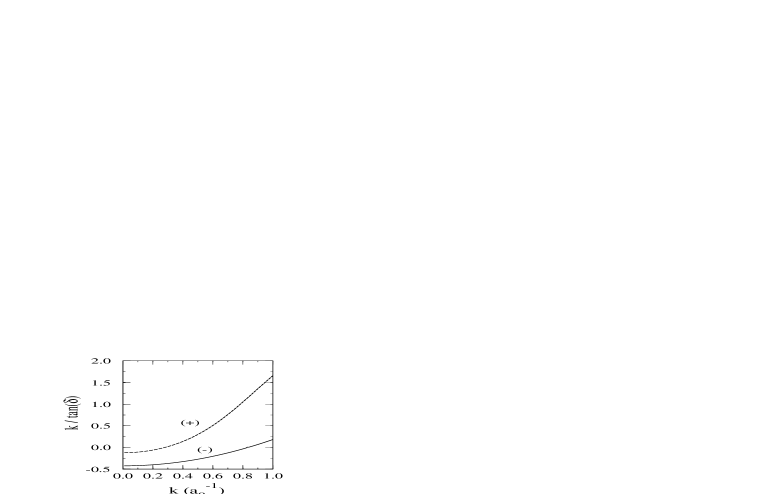
Figure 1: Dependence of the singlet (+) and triplet (-) $L=0$ phase shifts on the incident wave number, displayed in the form $k/\tan(\delta)$. Where these curves pass through zero, $\tan(\delta)$ goes through infinity, as is shown in the next two figures. Neither the M-IEM or the S-IEM had any difficulty evaluating these quantities either for the small values of $k$ or in the vicinity of the zeros.

The bench-test calculation performed by the three methods described above consists in obtaining the $L=0$ phase shift for the scattering of an electron from the ground-state of an Hydrogen atom, in the presence of exchange terms, both for the singlet and the triplet states, $\delta^{(+)}$ and $\delta^{(-)}$ , respectively. The methods are the S-IEM, the SVD, and the M-IEM. The older integral equation method is denoted as NIEM (the ”N” stands for non-iterative), and a representative result is taken from the paper by Sams and Kouri kouri , since these authors describe their accuracy for exactly the same test case as ours. The SVD, M-IEM and the NIEM methods use equi-spaced mesh points, since their auxiliary functions are the solutions of local differential equations using finite difference methods, while the S-IEM, as mentioned above, uses non-equispaced mesh points, which are the zeros of a Chebyshev polynomial of a certain order (16 in this case), in each of the partitions into which the radial interval is decomposed.

Figure 2: Momentum dependence of the singlet phase shift in the vicinity of $\pi/2$ (mod. $\pi$), as calculated by the S-IEM. Please note the scale of the y-axis.

The $k$ dependence of the phase shifts is shown in Fig. 1, by plotting the ratio $k/\tan(\delta).$ When either of the two curves crosses the $0$ line, the corresponding value of $\tan(\delta)$ becomes infinite,as is shown in Figs. (2) and (3), and the respective phases shift have the value $\pi/2,$ modulus $\pi.$ Both the M-IEM and the S-IEM methods had no difficulty in reproducing the singularity in $\tan(\delta),$ and both were able to reach arbitrarily small values of the momentum $k.$ By contrast, the SVD method could not obtain results for $k<1.0(a_{0})^{-1}.$

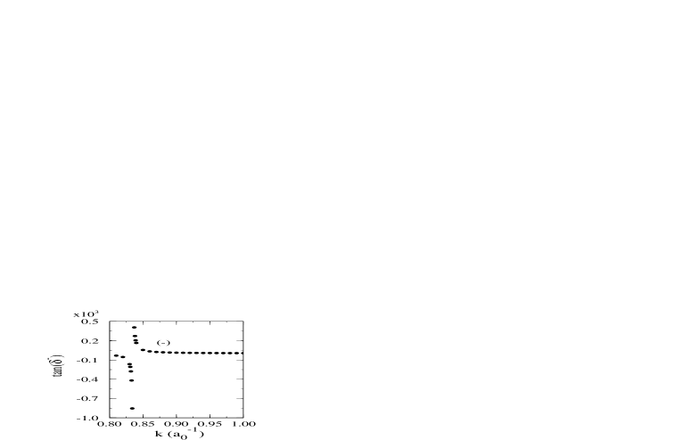
Figure 3: Same as Fig. 2 for the triplet phase shift.

Since well documented accuracy studies exist for the NIEM kouri we examined the rate of convergence of the phase shift as a function of number the mesh points for a case which is treated in Ref. kouri . The case chosen is the singlet phase shift with exchange, $\mathbf{\delta}^{(+)}$. The value of the wave number is $k=0.2\,(a_{0})^{-1}$ , and the maximum radial distance is $20\,a_{0}.$ The number of significant figures obtained for each of the non-spectral methods, all using a mesh size of 0.005 $a_{0},$ is shown in the three last rows of Table I. The result for the spectral method S-IEM, also shown.

Table 1: Accuracy of $\mathbf{\delta}^{(+)}$ for various algorithms.

Method	$\mathbf{\delta}^{(+)}$	# of Pts.
S-IEM	1.8701579	80
M-IEMa)	1.870156	4000
NIEM$\,{}^{b)}$	1.87015	4000
SVD	1.8701	4000

^a) Five basis states $D$ are used in this calculation

^b)Non-iterative method of Ref. kouri

The convergence of the four methods with the number of mesh-points is illustrated in Fig. 4. The number of significant figures for a given number of mesh points is determined from the stability of the result obtained after rounding, when compared to the result with the next higher number of points. It is clear from the figure that the S-IEM method reaches higher accuracy with a smaller number of points than the other methods shown. With 160 mesh points (the corresponding number of partitions is 10) the value obtained for $\delta^{(+)}=1.87015788462442$ rad. is the same , to within the quoted number of 15 significant figures, as the result for 224 mesh points. This is close to machine accuracy, and shows that the accumulation of round-off errors is small in the S-IEM method, confirming previous studies. (See Fig. 1 in the 1997 paper quoted in Ref. IEM ). The discrepancy in the seventh significant figure between the S-IEM and the M-IEM could be due to the fact that only five basis functions were used  for the latter. This point has not been investigated further.

The scattering length $a$ and effective range $r_{e}$ for this one state electron-hydrogen scattering calculation have also been examined. The procedure is similar to the one used for a previous atom-atom scattering bench-mark calculation IEMA . It is based on the low momentum expansion of the scattering phase shift

$$k\cot\delta_{0}=-\frac{1}{a}+r_{e}k^{2}+O(k^{3}).$$ (78)

The left hand side of the above expression is calculated for two very small values of the wave number $k$ , differing by a factor of two, and the values of $a$ and $r_{e}$ are solved for. The procedure is repeated for decreasing values of $k$ and increasing values of the maximum radial distance $r_{\max}$ and of the number of mesh-points until stability in the results is found to a given number of significant figures. For the values of $a$ and $r_{e}$ listed in the tables below for the S-IEM method, values of $k\approx 10^{-5}$ , $r_{\max}\approx 50$ and approximately $1000$ mesh points were found to be adequate. However, contrary to what was done in Ref. IEMA , the value of $r_{\max}$ was not extrapolated to $\infty$ via a perturbative method. For the M-IEM case, the values of $a$ and $r_{e}$ in Table IV are extracted from Eq. 78 by calculating $k\cot\delta_{0}$ for the two values of $k=0.00001$ and $0.01,$ and for $T=20.$ Excellent agreement with the S-IEM values is obtained.

Table II: Scattering lengths $a$.

Method	Singlet	No exchange	Triplet
S-IEM	8.100312397	-9.44716668854	2.349396156
M-IEM	8.1003	-9.44716	2.3494

Table III: Effective Range $r_{e}$.

Method	Singlet	No exch.	Triplet
S-IEM	1.51201	0.766797	0.6105
M-IEM	1.51	0.767	0.612

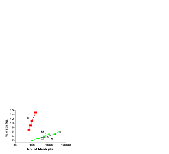
Figure 4: Comparison of the accuracy of the S-IEM, M-IEM and NIEM integral equation methods for the calculation of the singlet phase shift, as a function of the number of meshpoint used. The incident momentum is $k\,=0.2(a_{0})^{-1},$ and the value of the radial cut-off point is $r_{\max}=20\,a_{0}.$ The NIEM results are taken from Ref. kouri . The accuracy for a given number of mesh points of each method is determined by the number of significant figures which are stable (after rounding), as compared with the result for the next higher number of meshpoints.

VII Summary and Conclusions.

In this paper four methods were compared to solve the one-dimensional Schrödinger equation in the presence of the exchange nonlocality for the case of electron scattering from a hydrogen atom, with only the lowest energy state of the bound electron being included. The oldest method in the literature proceeds by first solving the equation in the presence of only the local potential, and then including the nonlocal part through Green’s function iteration. The iterations converge only for a limited range of parameters, and one of the methods described here improves upon the convergence by separating out of the nonlocal kernel a fully separable part by means of the Singular Value Decomposition method (SVD). By this means the region of convergence could be extended to a larger domain, but for our example convergence still fails at small values of the momentum, $k<0.1(a_{0})^{-1}$ and the maximum accuracy achieved was five significant figures. Another method was developed in the literature, in which the differential Schrödinger equation is first transformed into an Lippman-Schwinger integral equation, and is then solved non-iteratively (NIEM). In our example, taken from the literature kouri , this method achieved six significant figures of accuracy, but appears not to work for small values of the incident momentum. Improved accuracy and the viability for all values of $k$ was achieved in the present study by extending a previously developed spectral solution of a Lippman-Schwinger integral equation with local potentials IEM , IEMA , to the case with an exchange-type nonlocality. This extension was possible because the exchange nonlocality is of a semi-separable character. The resulting method (S-IEM) gives substantially higher accuracy (15 significant figures) than the NIEM, and converges much faster with the number of mesh-point in the integration interval than the NIEM, as is illustrated in Fig. 4. A fourth method, (M-IEM) developed previously for nonlocalities occurring in nuclear physics udagawa achieves seven figures of accuracy, and has no difficulty in coping with small values of $k.$ The rate of convergence of this method was comparable to that of the NIEM. The reason is due to the fact that the auxiliary functions needed for both methods, as well as the integration algorithms, are based on a finite difference algorithm, whose error usually decreases inversely with the number of mesh points according to a well defined power. From inspection of Fig. 4, this power has the relatively low value of 2.5. Both the M-IEM and the SVD methods have the advantage that they can be used for non-localities which are more general than the semi-separable exchange ones. The S-IEM also can be applied to these cases, but, at its present stage of development, the large matrix in Eq. 47 is then no longer sparse KKR .

In summary, four methods of calculating the scattering phase shift in electron atom collision were compared for a numerical test case, and the advantages and disadvantages of each were discussed.

Appendix 1

The relation between all coefficients in (46) can be written in the matrix form,

$$\left[\begin{array}[c]{cccc}M_{11}&M_{12}&M_{13}&M_{14}\\ M_{21}&M_{22}&M_{23}&M_{24}\\ M_{31}&M_{32}&M_{33}&M_{34}\\ M_{41}&M_{42}&M_{43}&M_{44}\end{array}\right]\left[\begin{array}[c]{c}\overline{\mathbf{A}}\\ \overline{\mathbf{B}}\\ \overline{\mathbf{C}}\\ \overline{\mathbf{D}}\end{array}\right]=\left[\begin{array}[c]{c}\overline{\mathbf{1}}\\ \overline{\mathbf{0}}\\ \overline{\mathbf{0}}\\ \overline{\mathbf{0}}\end{array}\right]\;\;\;eq:15$$ (79)

where

$${\bar{\mathbf{A}}} =[A_{1},...,A_{m}]^{T}\hskip 14.22636pt{\bar{\mathbf{B}}}=[B_{1},...,B_{m}]^{T},$$

$${\bar{\mathbf{C}}} =[C_{1},...,C_{m}]^{T}\hskip 14.22636pt{\bar{\mathbf{D}}}=[D_{1},...,D_{m}]^{T},$$

$${\bar{\mathbf{1}}} =[1,...,1]^{T}\hskip 14.22636pt\overline{\mathbf{0}}=[0,...,0]^{T},$$

and each of the block matrices $M_{ij}$ are either upper triangular matrices $U$ or lower triangular matrices $L$ with either $1^{\prime}s$ or $0^{\prime}s$ in the main diagonal, respectively (the subscripts are accordingly $1$ or $0$ ). These matrices $M_{i,j}$ are thus of the form

$$U_{1}=\left[\begin{array}[c]{ccccc}1&\gamma_{2}&\gamma_{2}&\cdots&\gamma_{m}\\ 0&1&\gamma_{3}&\cdots&\gamma_{m}\\ \vdots&&\ddots&&\vdots\\ 0&\cdots&0&1&\gamma_{m}\\ 0&\cdots&&0&1\end{array}\right],\;\;\;\;U_{0}=\left[\begin{array}[c]{ccccc}0&\gamma_{2}&\gamma_{2}&\cdots&\gamma_{m}\\ 0&0&\gamma_{3}&\cdots&\gamma_{m}\\ \vdots&&\ddots&&\vdots\\ 0&\cdots&0&0&\gamma_{m}\\ 0&\cdots&&0&0\end{array}\right]$$

or

$$L_{1}=\left[\begin{array}[c]{ccccc}1&0&\cdots&&0\\ \delta_{1}&1&\cdots&&0\\ \delta_{1}&\delta_{2}&1&\cdots&0\\ \vdots&\vdots&\ddots&1&0\\ \delta_{1}&\delta_{2}&\cdots&\delta_{m-1}&1\end{array}\right],\;\;\;\;L_{0}=\left[\begin{array}[c]{ccccc}0&0&\cdots&&0\\ \delta_{1}&0&\cdots&&0\\ \delta_{1}&\delta_{2}&0&\cdots&0\\ \vdots&\vdots&\ddots&0&0\\ \delta_{1}&\delta_{2}&\cdots&\delta_{m-1}&0\end{array}\right],$$

in which the entries $\gamma$ or $\delta$ are given in the table below

Using elementary row operations on equation (79) and then changing the order of the variables, the coefficient matrix of equation (79) can be transformed into the block tridiagonal system (47) to (49), given in the text. Further details can be found in Ref. IEM .

References

- (1) R. A. Gonzales, J. Eisert, I Koltracht, M. Neumann and G. Rawitscher, J. of Comput. Phys. 134, 134 (1997); R. A. Gonzales, S.-Y. Kang, I. Koltracht and G. Rawitscher, ibid 153, 160 (1999);
- (2) G. H. Rawitscher, B. D. Esry, E. Tiesinga, J. P. Burke, Jr., and I Koltracht, J of Chem. Phys. 111, 10418 (1999);
- (3) G. Rawitscher, I. Koltracht and I. Simbotin, Resonance Scattering as a test of a new highly accurate computational method, to be submitted for publication.
- (4) G. Rawitscher, S.-Y Kang and I. Koltracht, BAPS, 45, 18 (2000);
- (5) Sheon-Young Kang, Gauss Type Quadrature for Kernels with Discontinuities and Singularities and Applications, Ph.D. dissertation, University of Connecticut, Storrs, 2000.
- (6) I. Bray, Phys. Rev. Lett. 78, 4721 (1997);
- (7) S. Jones and A. T. Stelbovics, Phys. Rev. Lett. 84, 1878 (2000);
- (8) W. N. Sams and D. J. Kouri, J. Chem. Phys. 51, 4809 (1969).
- (9) B. T. Kim and T. Udagawa, Phys. Rev. C 42, 1147 (1990); T. Udagawa, Comp. Phys. Commun. 71, 150 (1992);
- (10) Essaid Zerrad, Ph. D. Thesis Generalization of the Hartree-Fock Approach to Atomic Collisions, University of Connecticut, 1998;
- (11) R. Kleinpoppen and U. Becker, Philos. Trans. R. Soc. Lond. A., Math. Phys. 357, 1229 (1999);
- (12) M. Joung et. al. Phys. Rev. Lett. 81, 1596 (1998);
- (13) B. C. Saha and C. A. Weatherford, J. Mol. Struct: THEOCHEM 388, 97 (1996);
- (14) E. O. Alt, A. S. Kadyrov and A. M. Mukhamedzhamov, Phys. Rev. A 60, 314 (1999);
- (15) C. Schwartz, Phys. Rev. 124, 1468 (1961); P. G. Burke and K. Smith, Rev. Mod. Phys., 34, 458 (1962); P. G. Burke, H. M. Schey and K. Smith, Phys. Rev. 129, 1258 (1963);
- (16) A. Temkin and J.C. Lamkin, Phys. Rev. 121, 788 (1961);
- (17) B. I. Schneider and L. A. Collins, Phys. Rev. A 24, 1264 (1981); L. A. Collins and B. I. Schneider, Phys. Rev. A 34, 1564 (1986);
- (18) Ed. R. Smith and R. J. Henry, Phys. Rev. A 7, 1585 (1973) and references therein; R. J. W. Henry, S. P. Rountree and Ed R. Smith, Comp. Phys. Comm., 23, 233 (1981);
- (19) R. Marriott, Proc. Roy. Soc. (London) 72, 121 (1958);
- (20) L. A. Collins and B. I. Schneider, J. Phys. B 14, L101 (1981); L. A. Collins and B. I. Schneider, Phys. Rev. A 24, 2387(1981);
- (21) C. A. Weatherford, K. Onda and A. Temkin, Phys. Rev. A 31, 3620 (1985);
- (22) I. Bray, Phys. Rev. A 49, 1066(1994) and references therein.
- (23) J. Macek, J. Phys. B, 1, 831 (1968); J. C. Y. Chen and I. Ishihara, Phys. Rev. 186, 25 (1969); G. H. Rawitscher, D. Lukaszek, R. S. Mackintosh and S. G. Cooper, Phys. Rev. C 49, 1621 (1994); R. Shakeshaft, Phys. Rev. A 62, 062705 (2000); D. Proulx, M. Pont and R. Shakeshaft, Pys. Rev. A 49, 1208 (1994);
- (24) J. Shertzer and J. Botero, Phys. Rev. A 49, 3673 (1994); C. A. Weatherford, M Dong and B. C. Saha, International Journal of Quantum Chemistry, S65, 591 (1997);
- (25) Atomic and Molecular Processes: an R-Matrix Approach, edited by P. G. Burke and K. A. Berrington (Institute of Physics, Bristol 1993); R. K. Nesbet, S. Mazevet and M. A. Morrison, Phys. Rev. A 64, 034702 (2001);
- (26) S.-Y Kang, I Koltracht and G. Rawitscher, Nystrom-Clenshaw-Curtis Quadrature for Integral Equations with Discontinuous Kernels, to appear in Mathematics of Computation;
- (27) D. R. Hartree, The Calculation of Atomic Structure, (Wiley, New York 1957), p 40; Kenneth Smith, The Calculation of Atomic Collision Processes, (Wiley Interscience, New York, 1971), p186 ff
- (28) H.Fiedeldey, R. Lipperheide, G, H, Rawitscher and S. A. Sofianos, Phys. Rev. C45, 2885 (1992).
- (29) G. H. Golub and C. H. Van Loan, Matrix Computations (Johns Hopkins University Press, Baltimore, 1983).
- (30) J. Stoer and R. Bulirsch. Introduction to Numerical Analysis, (English translation by R. Bartels, W. Gautchi and C. Witzgall). Springer-Verlag, New York, 1980; W. H. Press, S. A. Teukolsky, W. T. Vetteriling and B. P. Flannery. Numerical Recipes, The Art of Scientific Computing. Cambridge University Press, Cambridge, second edition, 1996.
- (31) R. R. Whitehead, A. Watt, B. J. Cole, and J. Morrison, Adv. Nucl. Phys. 9, 123 (1977).