The tunnel effect in electromagnetic propagation

Abstract

The tunnel effect is considered here within the framework of electromagnetic propagation. The classical problem of a plane gap of dielectric, surrounded on both sides by a medium with larger refraction index, is studied in the case in which an electromagnetic plane wave impinges into the gap with an incidence angle larger than the critical angle. In this condition (total reflection), the gap acts as a classically forbidden region and behaves like a tunnel. The field inside the forbidden gap consists of two evanescent waves, each one having its wavefronts normal to the interface. In the present paper we study the total field derived as a superposition of two such evanescent waves, its wavefronts, and the directions of propagation of both phase and energy.

In electromagnetism, an effect analogous to the tunnel effect of quantum mechanics occurs when a plane wave, propagating in a medium with refractive index $n$, impinges into a plane-parallel dielectric gap with refractive index $n^{\prime}$ smaller than $n$, at an incidence angle larger than the critical angle $i_{0}$ defined as $\sin i_{0}=n/n^{\prime}$. If the thickness $d$ of the gap is infinite, the field within the gap consists of a plane evanescent wave – attenuating in the direction normal to the interface – whose phase propagates in direction parallel to the interface (see Fig. 1a). If $d$ is finite, the boundary conditions on both interfaces cannot be satisfied by a single evanescent wave and two evanescent waves, with the same direction of propagation of the phase, but attenuating into opposite directions, are required (see Fig. 1b) [1].

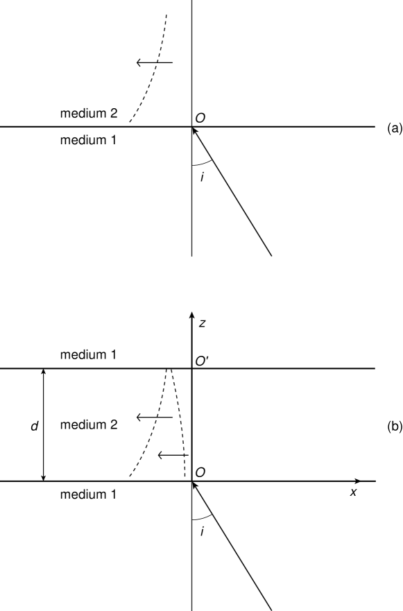
Figure 1: a) Border surface between medium 1, with refractive index $n^{\prime}$, and medium 2, with refractive index $n<n^{\prime}$. For an incidence angle $i$ larger than the critical angle $i_{0}=\arcsin(n/n^{\prime})$, a single evanescent wave originates in medium 2 and propagates parallel to the interface. b) Finite gap thickness of medium 1, surrounded on both sides by medium 2. In this case, two evanescent waves, with the same direction of propagation but attenuating into opposite directions, originate inside the gap. The width of the gap $d$ is shown, together with the coordinate system adopted in the theoretical analysis.

The properties of the total field inside the forbidden region are due to the fact that the two evanescent waves to be added have real amplitudes with opposite trends of variation in addition to the fact that the wavefronts, parallel to one another and normal to the interface, are not coinciding (on one wavefront the phase of a wave is different from the phase of the other wave, see Eqs.(5)). Accordingly, the phase of the total field varies along the wavefronts of the single waves to be added, and the wavefronts of the total field are not parallel to those of the component waves.

Let us consider a system of Cartesian coordinates $x,y,z$ (unit vectors of the axes i, j, k) with origin at $O$ (Fig. 1b), and an impinging TE wave with the electric field parallel to j, with direction of propagation s${}^{i}=(\alpha$i $+\gamma$k) in the plane $xz$. The $y$-component of the incident electric field can be written as

$$E^{i}=E_{0}\exp[ik_{0}n(\alpha x+\gamma z)]\>,$$ (1)

where $k_{0}=\omega/c$ is the free-space wavenumber, $E_{0}$ (which we assume to be real) denotes the amplitude of the incident field at the origin $O$ and

$$\gamma=\sqrt{1-\alpha^{2}}\>.$$

Inside the gap the total field is the superposition of two TE evanescent waves, whose electric field (still parallel to j) can be written as

$$E^{+} = pE_{0}\exp[k_{0}(in\alpha x-\Gamma z)]\exp(-i\omega t)\>,$$

$$E^{-} = rE_{0}\exp[k_{0}(in\alpha x+\Gamma z)]\exp(-i\omega t)\>,$$ (2)

where

$$\Gamma=\sqrt{n^{2}\alpha^{2}-1}$$

is a real quantity if, as assumed, the incidence angle is larger than the critical angle ($\alpha>1/n$).

The complex coefficients $p$ and $r$ can be deduced from the boundary conditions on the interfaces at $z=0$ and $z=d$[2]

$$p=\frac{e_{2}(\Gamma-in\gamma)}{2\Gamma}\,\tau=|p|\exp(i\varphi_{p})$$

$$r=\frac{e_{1}(\Gamma+in\gamma)}{2\Gamma}\,\tau=|r|\exp(i\varphi_{r})\>,$$ (3)

where

$$e_{1} = \exp(-k_{0}\Gamma d)\>,\>\>\>\>\>e_{2}=\frac{1}{e_{1}}=\exp(k_{0}\Gamma d)$$

$$\tau = |\tau|\exp(i\varphi_{\tau})=\frac{4in\gamma\Gamma}{e_{1}(\Gamma+in\gamma)^{2}-e_{2}(\Gamma-in\gamma)^{2}}$$ (4)

and

$$|p| = \frac{e_{2}}{2\Gamma}\,\Delta|\tau|\>,\>\>\>\>\>|r|=\frac{e_{1}}{2\Gamma}\,\Delta|\tau|$$

$$\varphi_{p} = \varphi_{\tau}-\Phi\>,\>\>\>\>\varphi_{r}=\varphi_{\tau}+\Phi$$

$$\Delta = \sqrt{\Gamma^{2}+n^{2}\gamma^{2}}=\sqrt{n^{2}-1}$$

$$\Phi = \arctan\left(\frac{n\gamma}{\Gamma}\right)\>.$$ (5)

From Eq. (5) it turns out that $\varphi_{p}$ and $\varphi_{r}$ differ by $2\Phi$. All the above quantities are independent of the coordinates, and $\tau$ represents the amplitude transmission coefficient of the gap[2]. The total electric field inside the gap can therefore be written as (apart from the time dependence $\exp(-i\omega t)$)

$$E^{g}=E^{+}+E^{-} = \frac{E_{0}\Delta|\tau|}{2\Gamma}\,\exp(ik_{0}n\alpha x)\times$$ (6)

$$\times \left[\frac{}{}\exp[k_{0}\Gamma(d-z)]\exp(i\varphi_{p})+\exp[-k_{0}\Gamma(d-z)]\exp(i\varphi_{r})\frac{}{}\right]$$

and, by taking into account Eq.(5), we have

$$E^{g} = \frac{E_{0}\Delta|\tau|}{2\Gamma}\,\exp(ik_{0}n\alpha x+i\varphi_{\tau})\times$$ (7)

$$\times \left[\frac{}{}\exp[k_{0}\Gamma(d-z)]\exp(-i\Phi)+\exp[-k_{0}\Gamma(d-z)]\exp(i\Phi)\frac{}{}\right]\>.$$

From Eq.(7) it turns out that the amplitude of $E^{g}$ depends only on $z$ (the equi-amplitude surfaces are the planes $z=$ constant), and decreases from the value $E_{0}\Delta|\tau|\sqrt{\cosh^{2}(k_{0}\Gamma d)-\sin^{2}\Phi}/\Gamma$, at $z=0$, to the value $E_{0}|\tau|$, at $z=d$. The spatial dependence of the amplitude implies that geometrical optics is inadequate for describing electromagnetic propagation within a tunneling region[3].

As to the phase, from Eq. (7) it follows that the equation of wavefronts (equi-phase surfaces) is given by

$$\varphi(x,z)=k_{0}n\alpha x+\Psi(z)+\varphi_{\tau}=\varphi_{0}\>,$$ (8)

where $\varphi_{0}$ is a constant and

$$\tan[\Psi(z)] = -\tanh[k_{0}\Gamma(d-z)]\tan(\Phi)=-\,\frac{n\gamma}{\Gamma}\tanh[k_{0}\Gamma(d-z)]$$

$$\varphi_{\tau} = \arctan\left[\frac{n^{2}\gamma^{2}-\Gamma^{2}}{2n\gamma\Gamma}\,\tanh(k_{0}\Gamma d)\right]\>.$$ (9)

Looking at Eq. (8), we can see that different wavefronts, corresponding to different values of the phase, are simply shifted in the $x$-direction with respect to one another. Figure 2 shows the wavefronts $\varphi_{0}=0,\pi,2\pi$ for parameter values referring to an experiment dealing with frustrated total reflection in the range of microwaves[4].

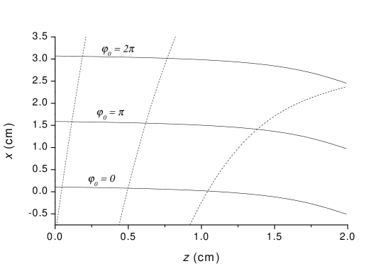
Figure 2: Wavefronts (solid lines) as derived from Eq. (8), for $\varphi_{0}=0,\>\pi,\>2\pi$, and rays (dashed lines) as derived from Eq. (17), for three arbitrary values of the constant $X_{0}$. The parameter values refer to an experimental situation[4] in which medium 1 consists of paraffin ($n^{\prime}=1.49$) and medium 2 of air ($n=1$). Other parameter values are: $\alpha=0.68,\>\nu=10\>{\rm GHz}\>(\omega=2\pi\nu),\>c=30\>{\rm cm/ns}$.

We can now derive both the wavelength and the equation of the rays. To this end, we have to evaluate grad$[\varphi(x,z)]$ and we have

$$\lambda=\frac{2\pi}{|{\rm grad}[\varphi(x,z)]|}$$ (10)

and, for the ray equation $x=X(z)$ defined as the lines of flux of grad$\varphi$,

$$\frac{dX}{dz}=\frac{(\partial\varphi/\partial x)}{(\partial\varphi/\partial z)}\>.$$ (11)

From Eq. (8) we have

$$\frac{\partial\varphi}{\partial x}=k_{0}n\alpha$$ (12)

$$\frac{\partial\varphi}{\partial z} = \frac{k_{0}\Gamma\sin\Phi\,\cos\Phi}{\cos^{2}\Phi\cosh^{2}[k_{0}\Gamma(d-z)]+\sin^{2}\Phi\sinh^{2}[k_{0}\Gamma(d-z)]}$$ (13)

$$= \frac{k_{0}\Gamma\sin\Phi\cos\Phi}{\cosh^{2}[k_{0}\Gamma(d-z)]-\sin^{2}\Phi}$$

hence

$$|{\rm grad}\,\varphi| = k_{0}\sqrt{n^{2}\alpha^{2}+\frac{\Gamma^{2}\sin^{2}\Phi\cos^{2}\Phi}{\left[\cosh^{2}[k_{0}\Gamma(d-z)]-\sin^{2}\Phi\right]^{2}}}$$ (14)

and

$$\frac{dX}{dz} = \frac{n\alpha}{\Gamma\sin\Phi\,\cos\Phi}\left[\cosh^{2}[k_{0}\Gamma(d-z)]-\sin^{2}\Phi\right]$$ (15)

$$= \frac{\alpha\Delta^{2}}{\gamma\Gamma^{2}}\left[\cosh^{2}[k_{0}\Gamma(d-z)]-\frac{n^{2}\gamma^{2}}{\Delta^{2}}\right]\>.$$

From Eq. (14) it follows that $|{\rm grad}\,\varphi|>k_{0}n\alpha$ and, from Eq. (10),

$$\lambda<\frac{\lambda_{0}}{n\alpha}<\lambda_{0},\>\>\>\>\>\>(n\alpha>1)$$ (16)

where $\lambda_{0}=2\pi/k_{0}$ is the free-space wavelength (medium 2 in Fig. 1). We can conclude, therefore, that the total field inside the tunneling region is slow, that is the phase velocity along the rays is slower than the light velocity $c$. By integrating Eq. (15), we obtain the ray equation

$$X(z)=\frac{\alpha\Delta^{2}}{\gamma\Gamma^{2}}\left[z\left(\frac{1}{2}-\frac{n^{2}\gamma^{2}}{\Delta^{2}}\right)-\frac{1}{4k_{0}\Gamma}\sinh[2k_{0}\Gamma(d-z)]\right]+X_{0}\>,$$ (17)

where $X_{0}$ is a constant. From Eq. (17), we can see that (as was to be expected due to the symmetries of the problem) the rays are shifted in the $x$-direction, and that, since the amplitude of the total field is not constant with respect to $z$, they are not straight lines (see Fig. 2).

By denoting the angle between a ray and the $z$-axis with $\chi$ ($\tan\chi=dX/dz$ (see Eq. (15)), we have, at $z=0$,

$$\sin\chi=\frac{\Delta^{2}\cosh^{2}(k_{0}\Gamma d)-n^{2}\gamma^{2}}{\sqrt{\left[\Delta^{2}\cosh^{2}(k_{0}\Gamma d)-n^{2}\gamma^{2}\right]^{2}+\left(\frac{\gamma\Gamma^{2}}{\alpha}\right)^{2}}}$$

while, at $z=d$,

$$\sin\chi=\alpha$$

Since $\chi$ is the refraction angle at $z=0$ and the incidence angle into the second interface at $z=d$, the unexpected conclusion is thus that the refraction low seems not to be valid for the rays inside the gap.

The Poynting vector inside the gap has a component normal to the interfaces, contrarily to what happens for the field on the right of the single interface of Fig. 1. In order to evaluate the flux lines of the Poynting vector and their relationship with the flux lines of the phase, let us consider the vector S describing the energy propogation[5]

$${\rm\bf S}=\frac{1}{2}{\rm Re}({\rm\bf E}\wedge{\rm\bf H}^{\star})\>,$$ (18)

where the asterix indicates a complex conjugate. We easily obtain

$$S_{x} = \frac{1}{2Z_{0}}n\alpha\,\left(\frac{E_{0}\Delta|\tau|}{\Gamma}\right)^{2}\left[\cosh^{2}[k_{0}\Gamma(d-z)]-\sin^{2}\Phi\right]$$

$$S_{z} = \frac{1}{2Z_{0}}n\gamma\,\left(E_{0}|\tau|\right)^{2}\>,$$ (19)

where $Z_{0}$ is the free space impedance. As expected, the $z$-component of the Poynting vector does not depend on $z$. The flux lines of the Poynting vector can therefore be written as

$$\frac{dx}{dz}=\frac{S_{x}}{S_{z}}=\frac{\alpha\Delta^{2}}{\gamma\Gamma^{2}}\left[\cosh^{2}[k_{0}\Gamma(d-z)]-\frac{n^{2}\gamma^{2}}{\Delta^{2}}\right]$$ (20)

and, by comparing this with Eq. (15), we see that the flux lines of the energy coincide with the flux lines of the phase.

By means of Eq. (8), we are able to evaluate the phase difference $\Delta\varphi$ between two opposite points, $O$ and $O^{\prime}$, along the $z$-direction inside the gap (see Fig. 1b): we have

$$\Delta\varphi=\varphi(0,d)-\varphi(0,0)=\arctan\left[\frac{n\gamma}{\Gamma}\tanh(k_{0}\Gamma d)\right]\>.$$

By including in the total phase also the temporal factor $\exp(-i\omega t)$ disregarded until now, the phase delay in going from $O$ (at $t=0$) to $O^{\prime}$ is

$$t_{\varphi}=\Delta\varphi/\omega.$$ (21)

In Fig. 3, we show $t_{\varphi}$ as a function of the gap width, together with the time $t_{l}=d/c$. If we suppose to perform an experiment (like the one reported in Ref. [4]) with a monocromatic wave and we put two probes at $O$ and $O^{\prime}$, we would actually measure a phase delay as given by Eq. (21) which is, without doubt, an observable[6]. To clarify the physical meaning of this delay we have to complete the analysis by considering not a plane wave impinging the gap, but a narrow beam or a wave packet[7, 8]. However, this improvement exceeds the purpose of the present work and will be presented elsewhere.

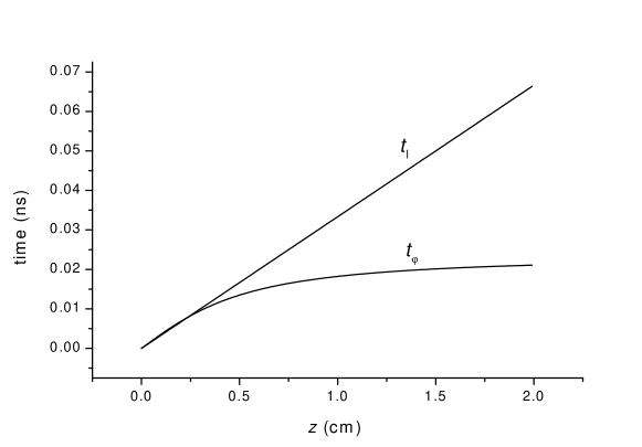
Figure 3: Phase delay time $t_{\varphi}$ along the $z$-direction as derived from Eq. (21), together with the time $t_{l}=z/c$, as a function of $z$. Parameter values are the same as those in Fig. 2.

Finally, we wish to note that $t_{\varphi}$ becomes independent on $d$, for large $d$ (see Eq. (21)). A behaviour of this kind was also obtained within the framework of a quantum-mechanical theoretical model, due to Hartman[9], for a particle tunneling through a rectangular potential barrier. Also in that case, the “traversal time” under barrier tends to be constant for large barriers, and the superluminal effect so obtained is known as ”Hartman effect”. It is not easy to understand the nature of that time but its behaviour, for large barrier, very similar to the one as derived here (Eq. (21)), could characterised it as a phase-delay[4, 10].

Acknowledgments

Thanks are due to L. Ronchi Abbozzo and A. Ranfagni for useful discussions and suggestions.

References

[1] The present treatment of the problem is different from that used by other authors who treat the internal field in terms of multiple reflections. See, for instance,
C. K. Carniglia and L. Mendel, J. Opt. Soc. Am. 61, (1971) 1035;
S. Zhu, A. W. Yu, D. Hawley, R. Roy, Am. J. Phys. 54, (1986) 601.
[2] D. Mugnai, A. Ranfagni, L. Ronchi, Atti della Fondazione
G. Ronchi 1 (1998) 777.
[3] G. Toraldo di Francia, La Diffrazione della Luce
(Einaudi, Torino, 1958) Chap II, Sec. 30.
[4] D. Mugnai, A. Ranfagni, L. Ronchi, Phys. Lett. A 247,
(1998) 281.
[5] G. Toraldo di Francia, Electromagnetic Waves (Interscience,
New York, 1955) Chap.III, Sec. 7.
[6]
From the boundary conditions, that is continuity conditions for the
tangential component of the electric fields across the interfaces,
at (in )
we have that the transmitted field is exactly equal to the internal field.
[7]
S. Bosanac, Phys. Rev. A 28, (1983) 577.
[8]
A. M. Steinberg and R. Y. Chiao, Phys. Rev. A 49, (1994) 3283.
[9]
T. E. Hartman, J. App. Phys. 33, (1962) 3427.
[10]
Besides the experiment reported in Ref. [4], another experimental work
where phase delay in a tunneling process is measured is:
D. Mugnai, A. Ranfagni, L. S. Schulman, Phys. Rev. E 55, (1997) 3593.