Evolution of Ultracold, Neutral Plasmas

Abstract

We present the first large-scale simulations of an ultracold, neutral plasma, produced by photoionization of laser-cooled xenon atoms, from creation to initial expansion, using classical molecular dynamics methods with open boundary conditions. We reproduce many of the experimental findings such as the trapping efficiency of electrons with increased ion number, a minimum electron temperature achieved on approach to the photoionization threshold, and recombination into Rydberg states of anomalously-low principal quantum number. In addition, many of these effects establish themselves very early in the plasma evolution ($\sim$ ns) before present experimental observations begin.

That a common characteristic connects such diverse environments as the surface of a neutron star, the initial compression stage of an inertial confinement fusion capsule, the interaction region of a high-intensity laser with atomic clusters, and a very cold, dilute, and partially-ionized gas within an atomic trap, seems at first rather remarkable. Yet all these cases embrace a regime known as a strongly-coupled plasma. For such a plasma, the interactions among the various constituents dominate the thermal motions. The plasma coupling constant $\Gamma_{\alpha}$, the ratio of the average electrostatic potential energy Z_α/a_α [ Z_α, the charge; a_α, the ion-sphere radius = $3$/($4\pi n_{\alpha}{{}^{1/3}})$; and $n_{\alpha}$, the number density for a given component $\alpha$] to the kinetic energy k_BT_α, provides an intrinsic measure of this effect [1]. When $\Gamma_{\alpha}$ exceeds unity, various strong-coupling effects commence such as collective modes and phase transitions. For multi-component plasmas, the coupling constants need not be equal or even comparable, leading to a medium that may contain both strongly- and weakly- coupled constituents.

Since temperatures usually start around a few hundred Kelvin, most plasmas found in nature or engineered in the laboratory attain strongly-coupled status from high densities, as in the case of a planetary interior or a shock-compressed fluid[2, 3], or from highly-charged states, as in colloidal or “dusty” plasmas [4]. In both situations, the particle density usually rises well above 10¹⁸/cm³. On the other hand, ion trapping and cooling methods have produced dilute, strongly-coupled plasmas by radically lowering the temperature. At first, these efforts were limited to nonneutral plasmas confined by a magnetic field[5]. However, recently, new techniques [6, 7, 8, 9] have generated neutral, ultracold plasmas, free of any external fields at densities of the order of 10⁸-10¹⁰/cm³ and temperatures at microkelvins ($\mu$K).

Two methods, one direct and one indirect, but both employing laser excitation of a highly-cooled sample of neutral atoms, have successfully created such neutral plasmas. The direct approach employs the photoionization of laser-cooled xenon atoms [6, 7, 8], while the indirect generates a cold Rydberg gas in which a few collisions with room-temperature atoms produces the ionization[9, 10]. In both cases, the electron and ion temperatures start very far apart with the former from 1K to 1000K and the latter remaining at the initial atom temperature of a few $\mu$K. This implies that the coupling constant for the electrons ($\Gamma_{e}$) ranges between 1 and 10, while the ions begin with $\Gamma_{i}\sim 1000$. Based on the results presented below, the following picture emerges. As the system evolves, the electrons reach a quasi-equilibrium while at the same time beginning to move the ions through long-range Coulomb interactions. Eventually, the ions also heat, and the whole cloud begins to expand with the ions and electrons approaching comparable temperatures. The former processes occur on the order of pico- to nano- seconds, while the full expansion becomes noticeable on a microsecond scale. Therefore, by following the progress of the system, we can study not only the basic properties of a strongly-coupled plasma but also its evolution through a variety of stages. The path to equilibration still remains a poorly understood process for strongly-coupled plasmas in general.

The dilute character of the ultracold plasmas provides a unique opportunity to explore the intricate nature of atomic-scale, strongly-coupled systems, both through real-time imaging of the sample to study wave phenomena, collective modes, and even phase transitions, and through laser probes to examine internal processes. The initial experiments have already discovered unexpected phenomena such as more rapid than expected ion expansion[7] and Rydberg populations that strongly deviate from those predicted from standard electron-ion recombination rates [8, 11, 12, 13]. So far, the experiments have examined the later expansion stage of the whole plasma cloud, which occurs on the scale of microseconds. However, the nature of the plasma at this stage depends strongly on its evolution from its creation. While ultra-fast laser techniques offer the eventual prospect of probing these early times, for now, only simulations can provide an understanding of the full evolution of these systems. We focus on the first such generated plasma[6] from the photoionization of cold Xenon atoms; however, the findings also provide insight into other ultracold systems.

Since the electron temperature greatly exceeds the Fermi temperature for this system, we may effectively employ a two-component classical molecular dynamics (MD) approach in which the electrons and ions are treated as distinguishable particles, interacting through a modified Coulomb potential. We have employed several different forms from an ab-initio Xe${}^{+}+e^{-}$ pseudopotential[14] to a simple effective cut-off potential[15] based on the de Broglie thermal wavelengths; we found little sensitivity of the basic properties to this choice. This finding stems from the dominance of the interactions by the very long-range Coulomb tails since the average particle separations are of the order of $10^{4}$Å(1 to 2 times the de Broglie wavelength for electrons at a temperature of 0.1K). The short-range modification of the Coulomb potential basically prevents particles with opposite charges from collapsing into a singularity. Due to the open and nonperiodic boundary conditions, sample size effects can play a critical role in the simulations[16]. Therefore, we must employ particle numbers of the basic order of the experiments, requiring efficient procedures for handling the long-range forces. In addition, the extended simulation times needed to model the entire plasma evolution [fs to $\mu$s] demand effective temporal treatments. To this end, we have employed multipole-tree procedures[17] in conjunction with reversible reference system propagator algorithms[18] (r-RESPA) through the parallel 3D MD program NAMD[19], generally used in biophysical applications. These procedures allow us to treat samples of between 10² and 10⁴ particles [N = N_i/2 = N_e/2]; most simulations were performed with N = 10³.

To reproduce the initial experimental conditions[6], we distribute the ions randomly according to a 3D Gaussian, whose rms radius, $\sigma$, matches the desired ion number density n_i [$\rm{n}_{i}=N_{i}/(2\pi\sigma^{2})^{3/2}$] and impose a Maxwell-Boltzmann velocity distribution at $T_{i}=1\mu$K. To each ion, we associate an electron placed randomly in an orbit of radius $r_{o}$= 50Å. The electron velocities point in random directions but with fixed magnitude, determined by the photoionization condition [K${}_{e}^{i}\equiv\frac{1}{2}m_{e}v_{e}^{2}=\hbar\omega-1/r_{o}$, with $\omega$, the laser frequency and $v_{e}^{2}$ as a sum over all three spatial components]. This idealized prescription models the photoionization process by allowing each electron to escape the Coulomb well with a final prescribed energy. By varying the laser frequency, we can control the final effective electron temperature, just as in the experiments. We tested this particular ionization model against simulations where both the initial electron-ion radius r_o and the form of the ion distribution are varied. Overall, we find little sensitivity to these variations on the basic initial conditions. Finally, we take a kinematic definition of temperature as the average kinetic energy per particle T_α = $\frac{1}{3N_{\alpha}k_{B}}\sum_{i}m_{\alpha}v_{\alpha,i}^{2}$, where the sum runs over all particles i of type $\alpha$.

The plasma evolves through several stages. In the first or photoionization stage, which lasts on the order of fs, the electrons climb out of the Coulomb well and become basically freely-moving particles. In the next stage, the electrons reach a quasi-equilibrium at T_e due to their fast intra-particle collisions. Following this stage, the electron-ion collisions begin the slow process of heating the ions, which can require up to $\mu$s. This process can also be viewed in terms of an electron pressure term in a hydrodynamical formulation[7]. Then, the whole cloud of ions and electrons begins a systematic expansion. This progression clearly evinces itself in Fig. 1, which shows the temporal behavior of electron and ion average kinetic energies, using an effective mass for the ion of m_i = 0.01 amu in order to accelerate the evolutionary process. The averaged kinetic energy of the electrons and ion become comparable and the cloud perceptibly expands in about 20 ns. Scaling this value by $\sqrt{\frac{m_{Xe}}{m_{i}}}$ yields an estimate for this time in a Xe plasma of about 1$\mu$s, in line with the experiments[6]. Also consistent with the experimental measurements[7], these preliminary calculations indicate that a large fraction of the kinetic energy transferred by the electrons results in outward translational motion for the ions. This implies that the kinetic temperature defined above coincides with the usual themodynamic temperature (random thermal motion) for the electrons only. In all other simulations discussed, the ions carry the mass of Xe.

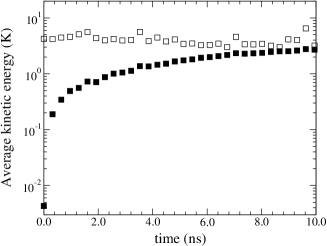
FIG. 1.: Schematic variation of the electron (open square) and ion (filled square) average kinetic energy per particle as a function of time for a model plasma with m_i=0.01 amu.

Since we shall use the simulations to understand intermediate stages in the development of the ultracold plasma, we need to establish the validity of the procedure by comparing to experiments. Two initial observations have particular significance: 1) the number of trapped electrons rises with the number of ions created for a fixed final temperature, and 2) the electrons attain a certain minimum temperature no matter how small $\hbar\omega$ becomes. Figure 2a shows that the number of trapped electrons as a function of the number of ions and initial electron temperature basically follows the general experimental trends[6]. Some of the electrons, freed by the photoionization process from ions with sufficient energy, escape the atomic cloud and never return, leaving an overall positively charged system. This residual charge then effectively traps the remaining electrons so that the center of the distribution resembles a neutral plasma. The larger the number of ions produced, the more effective the confinement of the electrons.

In Fig.2b, we present for n_i=4.32x10⁹ ions/cm³, the electron temperature T${}_{e}^{f}$ after the initial equilibration in the simulations as a function of the excess initial temperature T${}_{e}^{i}[=\frac{2}{3}K_{e}^{i}$] given to the electrons during the photoionization process. The plateau at about 5K [$\Gamma_{e}\sim 1$] for small T${}_{e}^{i}$ appears quite pronounced. This effect arises due to a mechanism usually designated as “continuum lowering”[1]. Despite the small energies and enormous distances involved, at least by usual atomic standards, the interaction of an ion with its neighbors still has a noticeable effect due to the very long-range of the Coulomb potential. This shifts the appropriate zero of energy from the isolated atom to the whole system. Using a simple binary interaction, we can estimate this energy difference for an electron halfway between the ions [$\sim 2/a_{ion}$] at around 3K for this density, in qualitative agreement with the simulations. Even for a photon energy near the atomic threshold, the electron within the plasma will still gain this minimum energy. This same effect also explains the dependence of the final electron temperature on the ion density. In this situation, an increase in the ion density enhances the zero of energy shift and leads to an increase in the final electron temperature.

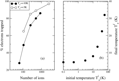
FIG. 2.: (a) Percentage of electrons trapped as a function of the number of ions created for two electron temperatures (3K and 10K). (b) Variation of the final electron temperature T${}_{e}^{f}$ as a function of the initial excess kinetic energy represented an associated temperature T${}_{e}^{i}$.

The molecular dynamics simulations yield additional properties of the ultracold plasma. We paid particular attention to the electron plasma frequency $f_{e}$ since experiments[7] have used this quantity as an indirect means of deducing the density of the ultracold plasma. Given the nature of the system with open boundary conditions and quasi-equilibration among the electrons, the question arises as to whether $f_{e}$ has a precise definition. Neglecting temperature dependence, the electron plasma frequency is given by

$$f_{e}=\frac{1}{2\pi}\sqrt{\frac{e^{2}n_{e}}{m_{e}}},$$ (1)

where e is the elementary charge, $n_{e}$ the electron density, and $m_{e}$ the electron mass. From the MD simulations, the electron plasma frequency is obtained from the Fourier transform of the electron velocity autocorrelation function[20]. We find, reassuringly, that a distinct though broadened peak arises near the $f_{e}$ predicted by Eq.1 in the regime in which the electrons reach a quasi-equilibration. For example, at a density of 4.32x10¹⁰ ions/cm³, an electron temperature of 3K, and simulation time extending up to 18ns, MD gives plasma frequencies of 1.2GHz (1.4 GHz) while Eq.1 yields 1.57GHz (1.87GHz) for trapped electrons at 70% (100%) of the ion density. When the ion density is decreased to a value of 4.32x10⁹ ions/cm³ at the same electron temperature, $f_{e}$ from the MD simulations becomes 0.5Ghz, also in accordance with Eq.1 . In general, we find that the number of particles used in the simulation cell has little effect on the determination of the electron plasma frequency beyond providing a better statistical sample.

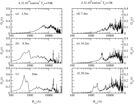
FIG. 3.: Time evolution of the modified ion-electron pair correlation function $G_{ie}$ as a function of density and electron temperature: (a)-(c) 4.32x10¹⁰ ions/cm³ and 10K, and (d)-(f) 4.32x10⁹ ions/cm³ and 3K.

We now turn to the nature of the constituents as the plasma evolves and pay particular attention to the formation of Rydberg atoms as noted in the experiments[8, 9, 10]. To this end, we examine over space and time the ion-electron pair correlation function $g_{ie}$(r), which gives the probability of finding an electron a distance r from a reference ion[15]. To enhance the examination of the closer encounters, we have employed a modified form $G_{ie}$(r) by subtracting a uniform distribution and averaging $g_{ie}$(r) over a small time interval of 1.5 ns. Figure 3 displays $G_{ie}$(r) for two representative cases. The open boundary conditions, which force the distribution to zero at some large distance, give $G_{ie}$(r) a distinctly different behavior than seen in a fluid or periodic system.

Figures 3(a)-(c) display the development of a plasma for n_i=4.32x10¹⁰ ions/cm³ and T${}_{e}\sim$ 10K in the regime in which the electrons have reached quasi-equilibration and the ions have started to heat. After 2.5ns, the electron distribution departs from its initial form, especially beyond a radius of 10000Å. By 8.5ns, we begin to observe an increase in $G_{ie}$ just below 1000Å. This signifies the formation of Rydberg states in an average principal quantum number n $\sim$ 40, a conclusion supported by an examination of movies of the simulation. These movies also show stable Rydberg atom configurations over many orbital periods of the electrons. A simple model[13] that balances various collisional processes, using strictly atomic cross sections, predicts a much larger value (n $\geq$ 100). For conditions closer to the experimental measurements (lower density), as depicted in Figs. 3(d)-(f), we find a significant Rydberg population after only 20ns (Fig.3f). The electron distribution shifts to around 2000Å, corresponding to a principal quantum number n $\sim$ 60. In both cases, the Rydberg population is estimated to be between 5% and 10 % of the total number of electrons. These findings closely resemble those of the experiments[8], though for later times ($\sim\mu$s) and indicate that collective or density effects may play an important role by changing the accessible Rydberg-level distribution or cross sections through long-range interactions. By examining the electron mean square displacement over time, we can identify two stages in the evolution of the cold ionized gas. First, after the ionization of the atoms, the electrons diffuse throughout the system for several nanoseconds with no significant Rydberg atom formation. Second, the electrons reach the edge of the cloud and begin systematic multiple traverses of the system. The Rydberg atom population becomes noticeable only several nanoseconds into this second stage. The feature that attracts the most interest is the relatively short time scale required to establish the neutral plasma and produce a noticeable Rydberg population.

In summary, we have followed the evolution of an ultracold, neutral plasma over a broad range of temporal stages with classical molecular dynamics simulation techniques. We find general agreement with experimental observations of the number of trapped electrons, the minimum of electron temperature, and the production of Rydberg atoms in low-lying states. The latter two conditions especially demonstrate the importance of strong-coupling or density effects on the basic atomic interactions. In addition, we have found that the electron plasma frequency appears as a valid tool to probe the state of the system. Important to the understanding of the temporal development of these plasmas, we discovered that recombination and the formation of long-lived Rydberg states occur rapidly on the order of nanoseconds. Our studies continue in an effort to push into the fully expanded regime by using hydrodynamical methods tied to the molecular dynamics.

We wish to acknowledge useful discussions with Dr. S. Rolston (NIST), Prof. T. Killian (Rice), and Prof. P. Gould (U. of Connecticut). We thank Dr. N. Troullier for providing the Xe pseudopotential. Work performed under the auspices of the U.S. Department of Energy (contract W-7405-ENG-36) through the Theoretical Division at the Los Alamos National Laboratory.

REFERENCES

- [1] S. Ichimaru, Statistical Plasma Physics, ed. Addison-Wesley, 1994.
- [2] W.J. Nellis et. al., Science 269,1249 (1995).
- [3] G. W. Collins et. al., Science 281(5380) 1178 (1998) and references therein.
- [4] M. Rosenberg, J. de Phys. IV, 10, 73 (2000) and references therein.
- [5] D.H.E. Dubin and T.M. O’Neil, Rev. Mod. Phys. 71, 87 (1999).
- [6] T.C. Killian et. al., Phys. Rev. Lett. 83, 4776 (1999).
- [7] S. Kulin et al., Phys. Rev. Lett., 85, 318 (2000).
- [8] T.C. Killian et. al., Phys. Rev. Lett. 86, 3759 (2001).
- [9] M.P. Robinson et. al., Phys. Rev. Lett. 85, 4466, (2000).
- [10] P. Gould and E. Eyler, Phys. World 14, 19-20 (2001).
- [11] D.R. Bates et. al. Proc. R. Soc. London A 267, 297 (1962).
- [12] Y. Hahn, Phys. Lett. A 231, 82 (1997); Phys. Lett. A 264, 465 (2000).
- [13] J. Stevefelt et. al. Phys. Rev. A 12, 1246 (1975).
- [14] N. Troullier and J.L. Martins, Phys. Rev. B 43, 1993 (1991).
- [15] J.P. Hansen and I.R. McDonald, Phys. Rev. A 23, 2041 (1981).
- [16] Far more restrictive calculations using periodic boundary conditions have been reported by A. Tkackev et al., Quant. Elect. 30, 1077 (2000) and, after submission of this article, by M. Morrillo Phys. Rev. Let. 87, 115003-1 (2001).
- [17] L. Greengard and V. Rokhlin, J. Comp. Phys. 73, 325 (1987); J. Barnes and P. Hut, Nature 324, 446 (1986).
- [18] F. Figueirido et. al., J. Chem. Phys. 106, 9835 (1997) and references therein.
- [19] L. Kale et. al., J. Comp. Phys.151, 283-312 (1999).
- [20] J.P. Hansen, and I. McDonald, Theory of Simple liquid, ed. Academic Press (1986).