Bayesian inference for inverse problems

Abstract

Traditionally, the MaxEnt workshops start by a tutorial day. This paper summarizes my talk during 2001’th workshop at John Hopkins University. The main idea in this talk is to show how the Bayesian inference can naturally give us all the necessary tools we need to solve real inverse problems: starting by simple inversion where we assume to know exactly the forward model and all the input model parameters up to more realistic advanced problems of myopic or blind inversion where we may be uncertain about the forward model and we may have noisy data.

Starting by an introduction to inverse problems through a few examples and explaining their ill posedness nature, I briefly presented the main classical deterministic methods such as data matching and classical regularization methods to show their limitations. I then presented the main classical probabilistic methods based on likelihood, information theory and maximum entropy and the Bayesian inference framework for such problems. I show that the Bayesian framework, not only generalizes all these methods, but also gives us natural tools, for example, for inferring the uncertainty of the computed solutions, for the estimation of the hyperparameters or for handling myopic or blind inversion problems. Finally, through a deconvolution problem example, I presented a few state of the art methods based on Bayesian inference particularly designed for some of the mass spectrometry data processing problems.

1 Introduction

1.1 Forward and inverse problems

In experimental science, it is hard to find an example where we can measure directly a desired quantity. Describing mathematical models to relate the measured quantities to the unknown quantity of interest is called forward modeling problem. The main object of a forward modeling is to be able to generate data which are as likely as possible to the observed data if the unknown quantity was known. But, almost always, we want to use this model and the observed data to make inference on the unknown quantity of interest: This is the inversion problem. To be more explicit, let take an example that we will use all along this paper to illustrate the different aspects of inverse problems. The example is taken from the mass spectrometry where the ideal physical quantity of interest is the components mass distribution of the material under the test. There are many techniques used in mass spectrometry. The Time-of-Flight (TOF) technique is one of them. In this technique, one measures the electrical current generated on the surface of a detector by the charged ions generated by the material under the test. Finding a very fine physical model to relate the time variation of this current to the distribution of the arrival times of the charged ions, which is itself related to the components mass distribution of the material under the test, is not an easy task. However, in a first approximation, assuming that the instrument is linear and its characteristics do not change during the acquisition time of the experiment, a very simple convolution model relates the raw data $g(t)$ to the unknown quantity of interest $f(t)$:

$$g(\tau)=\int f(t)\,h(\tau-t){\;\mbox{d}t},$$ (1)

where $h(t)$ is the point spread function (psf) of the instrument. Figure 1 shows an example of data observed (signal in b) for a theoretical mass distribution (signal in a).

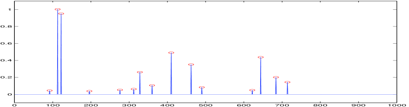
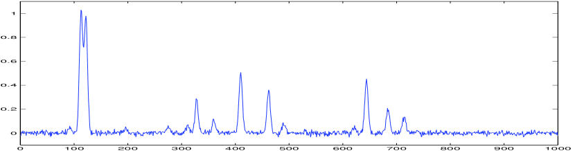
Figure 1: Blurring effect in TOF mass spectrometry data:   a) desired or theoretical spectrum,   b) observed data.

In this example, the forward problem consists in computing $g$ given $f$ and $h$ which is given by a simple convolution operation. The inverse problem of inferring $f$ given $g$ and $h$ is called deconvolution, the inverse problem of inferring $h$ given $g$ and $f$ is called psf identification and the inverse problem of inferring $h$ and $f$ given only $g$ is called blind deconvolution.

In my talk, I have given many more examples such as image restoration

$$g(x^{\prime},y^{\prime})=\int\int f(x,y)\,h(x^{\prime}-x,y^{\prime}-y){\;\mbox{d}x}{\;\mbox{d}y},$$ (2)

or Fourier synthesis inversion

$$g(\tau)=\int f(\omega)\,\exp\left\{-j\omega\tau\right\}{\;\mbox{d}\omega}$$ (3)

as well as a few non linear inverse problems. I am not going to detail them here, but I try to give a unified method to deal with all these problems. For this purpose, first we note that, in all these problems, we have always limited the number of data, for example $y_{i}=g(\tau_{i}),\;i=1,\ldots,m$. We also note that, to be able to do numerical computation, we need to model the unknown function $f$ by a finite number of parameters ${\mbox{\boldmath$x$}}=[x_{1},\ldots,x_{n}]$. As an example, we may assume that

$$f(t)=\sum_{j=1}^{n}x_{j}b_{j}(t)$$ (4)

where $b_{j}(t)$ are known basis functions. With this assumption the raw data ${\mbox{\boldmath$y$}}=[y_{1},\ldots,y_{m}]$ are related to the unknown parameters $x$ by

$$y_{i}=g(\tau_{i})=\sum_{j=1}^{n}H_{i,j}\,x_{j}\mbox{~{}~{}~{}with~{}~{}~{}}H_{i,j}=\int\kern-11.00008pt\int b_{j}(t)h(t-\tau_{i}){\;\mbox{d}t}$$ (5)

which can be written in the simple matrix form ${\mbox{\boldmath$y$}}={\mbox{\boldmath$H$}}{\mbox{\boldmath$x$}}$. The inversion problem can then be simplified to the estimation of $x$ given $H$ and $y$. Two approaches are then in competition:
i) the dimensional control approach which consists in an appropriate choice of the basis functions $b_{j}({\mbox{\boldmath$r$}})$ and $n\leq m$ in such a way that the equation ${\mbox{\boldmath$y$}}={\mbox{\boldmath$A$}}{\mbox{\boldmath$x$}}$ be well conditioned;
ii) the more general regularization approach where a classical sampling basis for $b_{j}({\mbox{\boldmath$r$}})$ with desired resolution is chosen no matter if $n>m$ or if $A$ is ill conditioned. In the following, we follow the second approach which is more flexible for adding more general prior information on $x$.

We must also remark that, in general, it is very difficult to give a very fine mathematical model to take account for all the different quantities affecting the measurement process. However, we can almost always come up with a more general relation such as

$$y_{i}={\mbox{\boldmath$h$}}_{{\mbox{\boldmath$\theta$}}}({\mbox{\boldmath$x$}})+\epsilon_{i},\quad i=1,\ldots,m$$ (6)

where $\theta$ represents the unknown parameters of the forward model (for example the amplitude and the width of a Gaussian shape psf in a deconvolution problem) and ${\mbox{\boldmath$\epsilon$}}=[\epsilon_{1},\ldots,\epsilon_{m}]$ represents all the errors (measurement noise, discretization errors and all the other uncertainties of the model). For the case of linear models we have

$${\mbox{\boldmath$y$}}={\mbox{\boldmath$H$}}_{{\mbox{\boldmath$\theta$}}}{\mbox{\boldmath$x$}}+{\mbox{\boldmath$\epsilon$}}.$$ (7)

In this paper we focus on this general problem. We first consider the case where the model is assumed to be perfectly known. This is the simple inversion problem. Then we consider the more general case where we have also to infer on $\theta$. This is the myopic or blind inversion problem.

Even in the simplest case of perfectly known linear system and exact data:
i) the operator $H$ may not be invertible (${\mbox{\boldmath$H$}}^{-1}$ does not exist);
ii) it may admit more than one inverse ($\exists{\mbox{\boldmath$G$}}_{1}\mbox{~{}and~{}}{\mbox{\boldmath$G$}}_{2}|{\mbox{\boldmath$G$}}_{1}({\mbox{\boldmath$H$}})={\mbox{\boldmath$G$}}_{2}({\mbox{\boldmath$H$}})={\mbox{\boldmath$I$}}$ where $I$ is the identity operator); or
iii) it may be very ill-posed or ill-conditioned (meaning that there exists $x$ and ${\mbox{\boldmath$x$}}+\alpha\delta{\mbox{\boldmath$x$}}$  for which  $\left\|{\mbox{\boldmath$H$}}^{-1}({\mbox{\boldmath$x$}})-{\mbox{\boldmath$H$}}^{-1}({\mbox{\boldmath$x$}}+\alpha\delta{\mbox{\boldmath$x$}})\right\|$  never vanishes even if $\alpha\mapsto 0$ Bertero88a ; Demoment89 .

These are the three necessary conditions of existence, uniqueness and stability of Hadamard for the well-posedness of an inversion problem. This explains the fact that, in general, even in this simple case, many naïve methods based on generalized inversion or on least squares may not give satisfactory results. The following figure shows, in a simple way, the ill-posedness of a deconvolution problem. On this figure, we see that three different input signals can result three outputs which are practically indistinguishable from each other. This means that, data matching alone can not distinguish between any of these inputs.

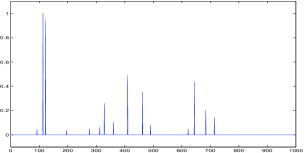
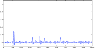
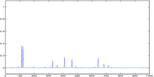
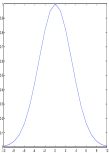
$\longrightarrow$ $\longrightarrow$

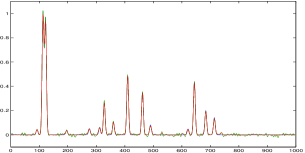
Figure 2: Ill-posedness of a deconvolution problem: Inputs on the left give practically indistinguishable outputs.

As a conclusion, we see that, apart from the data, we need extra information. The art of inversion in a particular inverse problem is how to include just enough prior information to obtain a satisfactory result. In the following, first we summarize the classical deterministic approaches of data matching and regularization. Then, we focus on probabilistic approaches where errors and uncertainties are taken into account through the probability laws. Here, we distinguish, three classes of methods: those which only account for the data errors (error probability distribution matching and likelihood based methods), those which only account for uncertainties of unknown parameters (entropy based methods) and those which account for both of them (Bayesian inference approach).

2 Data matching and regularization methods

2.1 Exact data matching

Let consider the discretized equation $y_{i}=h_{i}({\mbox{\boldmath$x$}})+\epsilon_{i},\;i=1,\ldots,m$; and assume first that the model and data are exact ($\epsilon_{i}=0$). We can then write ${\mbox{\boldmath$y$}}={\mbox{\boldmath$h$}}({\mbox{\boldmath$x$}})$.

Assume now the system of equations is under determined, i.e., there is more than one solution satisfying it (for example when the number of data is less than the number of unknowns). Then, one way to obtain a unique solution is to define an a priori criterion, for example $\Delta({\mbox{\boldmath$x$}},{\mbox{\boldmath$m$}})$ to choose that unique solution by

$$\widehat{{\mbox{\boldmath$x$}}}=\mathop{\mbox{arg}\min}_{{\mbox{\boldmath$h$}}({\mbox{\boldmath$x$}})={\mbox{\boldmath$y$}}}\left\{{\Delta({\mbox{\boldmath$x$}},{\mbox{\boldmath$m$}})}\right\}$$ (8)

where $m$ is an a priori solution and $\Delta$ a distance measure.

In the linear inverse problems case, the solution to this constrained optimization can be obtained via Lagrangian techniques which consists in defining the Lagrangian $\mbox{$\cal L$}({\mbox{\boldmath$x$}},{\mbox{\boldmath$\lambda$}})=\Delta({\mbox{\boldmath$x$}},{\mbox{\boldmath$m$}})+{\mbox{\boldmath$\lambda$}}^{t}({\mbox{\boldmath$y$}}-{\mbox{\boldmath$H$}}{\mbox{\boldmath$x$}})$ and searching for $(\widehat{{\mbox{\boldmath$\lambda$}}},\widehat{{\mbox{\boldmath$x$}}})$ through

$$\left\{\begin{array}[]{lcl}\widehat{{\mbox{\boldmath$\lambda$}}}&=&\mathop{\mbox{arg}\min}_{{\mbox{\boldmath$\lambda$}}}\left\{{\mbox{$\cal D$}({\mbox{\boldmath$\lambda$}})=\inf_{{\mbox{\boldmath$x$}}}\mbox{$\cal L$}({\mbox{\boldmath$x$}},{\mbox{\boldmath$\lambda$}})}\right\}\\ \widehat{{\mbox{\boldmath$x$}}}&=&\mathop{\mbox{arg}\min}_{{\mbox{\boldmath$x$}}}\left\{{\mbox{$\cal L$}({\mbox{\boldmath$x$}},\widehat{{\mbox{\boldmath$\lambda$}}})}\right\}\end{array}\right.$$ (9)

Noting that $\nabla_{{\mbox{\boldmath$x$}}}\mbox{$\cal L$}=\nabla_{{\mbox{\boldmath$x$}}}\Delta({\mbox{\boldmath$x$}},{\mbox{\boldmath$m$}})-{\mbox{\boldmath$H$}}^{t}{\mbox{\boldmath$\lambda$}}$ and $\nabla_{{\mbox{\boldmath$\lambda$}}}\mbox{$\cal L$}={\mbox{\boldmath$y$}}-{\mbox{\boldmath$H$}}{\mbox{\boldmath$x$}}$ and defining $\mbox{$\cal G$}({\mbox{\boldmath$s$}},{\mbox{\boldmath$m$}})=\sup_{{\mbox{\boldmath$x$}}}\{{\mbox{\boldmath$x$}}^{t}{\mbox{\boldmath$s$}}-\Delta({\mbox{\boldmath$x$}},{\mbox{\boldmath$m$}})\}$ the algorithm to find the solution $\widehat{{\mbox{\boldmath$x$}}}$ becomes:
– Determine $\mbox{$\cal G$}({\mbox{\boldmath$s$}},{\mbox{\boldmath$m$}})=\sup_{{\mbox{\boldmath$x$}}}\{{\mbox{\boldmath$x$}}^{t}{\mbox{\boldmath$s$}}-\Delta({\mbox{\boldmath$x$}},{\mbox{\boldmath$m$}})\}$;
– Find $\widehat{{\mbox{\boldmath$\lambda$}}}=\mathop{\mbox{arg}\min}_{{\mbox{\boldmath$\lambda$}}}\left\{{\mbox{$\cal D$}({\mbox{\boldmath$\lambda$}})={\mbox{\boldmath$\lambda$}}^{t}{\mbox{\boldmath$y$}}-\mbox{$\cal G$}({\mbox{\boldmath$H$}}^{t}{\mbox{\boldmath$\lambda$}},{\mbox{\boldmath$m$}})}\right\}$;
– Determine $\widehat{{\mbox{\boldmath$x$}}}=\nabla_{{\mbox{\boldmath$s$}}}\mbox{$\cal G$}({\mbox{\boldmath$H$}}^{t}\widehat{{\mbox{\boldmath$\lambda$}}})$.

As an example, when $\Delta({\mbox{\boldmath$x$}},{\mbox{\boldmath$m$}})=\frac{1}{2}\left\|{\mbox{\boldmath$x$}}-{\mbox{\boldmath$m$}}\right\|^{2}$ then $\mbox{$\cal G$}({\mbox{\boldmath$s$}},{\mbox{\boldmath$m$}})={\mbox{\boldmath$m$}}^{t}{\mbox{\boldmath$s$}}+\frac{1}{2}\left\|{\mbox{\boldmath$s$}}\right\|^{2}$, $\nabla_{{\mbox{\boldmath$s$}}}\mbox{$\cal G$}={\mbox{\boldmath$m$}}+{\mbox{\boldmath$s$}}$ and $\mbox{$\cal D$}({\mbox{\boldmath$\lambda$}})={\mbox{\boldmath$\lambda$}}^{t}{\mbox{\boldmath$y$}}-{\mbox{\boldmath$m$}}^{t}{\mbox{\boldmath$H$}}^{t}{\mbox{\boldmath$\lambda$}}+\frac{1}{2}\left\|{\mbox{\boldmath$H$}}^{t}{\mbox{\boldmath$\lambda$}}\right\|^{2}$ which results to $\widehat{{\mbox{\boldmath$\lambda$}}}=({\mbox{\boldmath$H$}}{\mbox{\boldmath$H$}}^{t})^{-1}({\mbox{\boldmath$y$}}-{\mbox{\boldmath$H$}}{\mbox{\boldmath$m$}})$ and the solution is given by

$$\widehat{{\mbox{\boldmath$x$}}}={\mbox{\boldmath$m$}}+{\mbox{\boldmath$H$}}^{t}({\mbox{\boldmath$H$}}{\mbox{\boldmath$H$}}^{t})^{-1}({\mbox{\boldmath$y$}}-{\mbox{\boldmath$H$}}{\mbox{\boldmath$m$}}).$$ (10)

One can remark that, when ${\mbox{\boldmath$m$}}=\mbox{\boldmath$0$}$ we have $\widehat{{\mbox{\boldmath$x$}}}={\mbox{\boldmath$H$}}^{t}({\mbox{\boldmath$H$}}{\mbox{\boldmath$H$}}^{t})^{-1}{\mbox{\boldmath$y$}}$ and this is the classical minimum norm generalized inverse solution.

Another example is the classical Maximum Entropy method case where $\Delta({\mbox{\boldmath$x$}},{\mbox{\boldmath$m$}})=\mbox{KL}({\mbox{\boldmath$x$}},{\mbox{\boldmath$m$}})$ is the Kullback-Leibler distance or cross entropy between $x$ and the a priori solution $m$:

$$\mbox{KL}({\mbox{\boldmath$x$}},{\mbox{\boldmath$m$}})=\sum_{j}x_{j}\ln\frac{x_{j}}{m_{j}}-(x_{j}-m_{j})$$ (11)

Here, the solution is given by

$$\widehat{x}_{j}=m_{j}\exp\left[{-[{\mbox{\boldmath$A$}}^{t}\widehat{{\mbox{\boldmath$\lambda$}}}]_{j}}\right]\mbox{~{}with~{}}\widehat{{\mbox{\boldmath$\lambda$}}}=\mathop{\mbox{arg}\min}_{{\mbox{\boldmath$\lambda$}}}\left\{{\mbox{$\cal D$}({\mbox{\boldmath$\lambda$}})={\mbox{\boldmath$\lambda$}}^{t}{\mbox{\boldmath$y$}}-\mbox{$\cal G$}({\mbox{\boldmath$A$}}^{t}{\mbox{\boldmath$\lambda$}},{\mbox{\boldmath$m$}})}\right\}$$ (12)

where $\mbox{$\cal G$}({\mbox{\boldmath$s$}},{\mbox{\boldmath$m$}})=\sum_{j}m_{j}\left(1-\exp\left[{-s_{j}}\right]\right)$. But, unfortunately here $\mbox{$\cal D$}({\mbox{\boldmath$\lambda$}})$ is not a quadratic function of $\lambda$ and thus there is not an analytic expression for $\widehat{{\mbox{\boldmath$\lambda$}}}$. However, it can be computed numerically and many algorithms have been proposed for its efficient computation. See for example Skilling84 and the cited references for more discussions on the computational issues and algorithm implementation.

The main issue here is that, this approach gives a satisfactory solution to the uniqueness of the inverse problem, but in general, the performances obtained by the resulting algorithms stay sensitive to error on the data.

2.2 Least squares data matching and regularization

When the discretized equation ${\mbox{\boldmath$y$}}={\mbox{\boldmath$h$}}({\mbox{\boldmath$x$}})$ is over-determined, i.e., there is no solution satisfying it exactly (for example when the number of data is greater than the number of unknowns or when the data are not exact), one can try to estimate them by:

$$\widehat{{\mbox{\boldmath$x$}}}=\mathop{\mbox{arg}\min}_{{\mbox{\boldmath$x$}}}\left\{{\Delta({\mbox{\boldmath$y$}},{\mbox{\boldmath$h$}}({\mbox{\boldmath$x$}}))}\right\},$$ (13)

where $\Delta({\mbox{\boldmath$y$}},{\mbox{\boldmath$h$}}({\mbox{\boldmath$x$}}))$ is a distance measure in the data space. The case where $\Delta({\mbox{\boldmath$y$}},{\mbox{\boldmath$h$}}({\mbox{\boldmath$x$}}))=\left\|{\mbox{\boldmath$y$}}-{\mbox{\boldmath$h$}}({\mbox{\boldmath$x$}})\right\|^{2}$ is the classical Least Squares (LS) criterion.

For a linear inversion problem ${\mbox{\boldmath$y$}}={\mbox{\boldmath$H$}}{\mbox{\boldmath$x$}}$, it is easy to see that any $\widehat{{\mbox{\boldmath$x$}}}$ which satisfies the normal equation ${\mbox{\boldmath$H$}}^{t}{\mbox{\boldmath$H$}}\widehat{{\mbox{\boldmath$x$}}}={\mbox{\boldmath$H$}}^{t}{\mbox{\boldmath$y$}}$ is a LS solution. If ${\mbox{\boldmath$H$}}^{t}{\mbox{\boldmath$H$}}$ is invertible and well-conditioned then $\widehat{{\mbox{\boldmath$x$}}}=({\mbox{\boldmath$H$}}^{t}{\mbox{\boldmath$H$}})^{-1}{\mbox{\boldmath$H$}}^{t}{\mbox{\boldmath$y$}}$ is again the unique generalized inverse solution. But, in general, this is not the case: ${\mbox{\boldmath$H$}}^{t}{\mbox{\boldmath$H$}}$ is rank deficient and we need to constrain the space of the admissible solutions. The constraint LS is then defined as

$$\widehat{{\mbox{\boldmath$x$}}}=\mathop{\mbox{arg}\min}_{{\mbox{\boldmath$x$}}\in\mbox{$\cal C$}}\left\{{\left\|{\mbox{\boldmath$y$}}-{\mbox{\boldmath$H$}}{\mbox{\boldmath$x$}}\right\|^{2}}\right\}.$$ (14)

where $\cal C$ is a convex set. The choice of the set $\cal C$ is primordial to satisfy the three conditions of a well-posed solution. An example is the positivity constraint: $\mbox{$\cal C$}=\{{\mbox{\boldmath$x$}}:\;\forall j,\;x_{j}>0\}$. Another example is $\mbox{$\cal C$}=\{{\mbox{\boldmath$x$}}:\;\left\|{\mbox{\boldmath$x$}}\right\|<\alpha\}$ where the solution can be computed via the optimization of

$$J({\mbox{\boldmath$x$}})=\left\|{\mbox{\boldmath$y$}}-{\mbox{\boldmath$H$}}({\mbox{\boldmath$x$}})\right\|^{2}+\lambda\left\|{\mbox{\boldmath$x$}}\right\|.$$ (15)

The main technical difficulty is the relation between $\alpha$ and $\lambda$. The minimum norm LS solution can also be computed using the singular value decomposition Hanson71 . The main issue here is that, even if this approach has been well understood and commonly used, it assumes implicitly that the noise and the $x$ are Gaussian. This may not be suitable in some applications, and more specifically in mass spectrometry data processing where the unknowns are spiky spectra.

A more general regularization procedure is to define the solution to the inversion problem ${\mbox{\boldmath$y$}}={\mbox{\boldmath$H$}}({\mbox{\boldmath$x$}})+{\mbox{\boldmath$\epsilon$}}$ as the optimizer of a compound criterion $J({\mbox{\boldmath$x$}})=\left\|{\mbox{\boldmath$y$}}-{\mbox{\boldmath$H$}}{\mbox{\boldmath$x$}}\right\|^{2}+\lambda\phi({\mbox{\boldmath$x$}})$ or the more general criterion

$$J({\mbox{\boldmath$x$}})=\Delta_{1}({\mbox{\boldmath$y$}},{\mbox{\boldmath$H$}}{\mbox{\boldmath$x$}})+\lambda\Delta_{2}({\mbox{\boldmath$x$}},{\mbox{\boldmath$m$}}).$$ (16)

where $\Delta_{1}$ and $\Delta_{2}$ are two distances or discrepancy measures, $\lambda$ a regularization parameter and $m$ an a priori solutionIdier96a . The main questions here are: i) how to choose $\Delta_{1}$ and $\Delta_{2}$ and ii) how to determine $\lambda$ and $m$.

For the first question, many choices exist:
– Quadratic or $L_{2}$ distance: $\Delta({\mbox{\boldmath$x$}},{\mbox{\boldmath$z$}})=\left\|{\mbox{\boldmath$x$}}-{\mbox{\boldmath$z$}}\right\|^{2}=\sum_{j}(x_{j}-z_{j})^{2}$;
– $L_{p}$ distance: $\Delta({\mbox{\boldmath$x$}},{\mbox{\boldmath$z$}})=\left\|{\mbox{\boldmath$x$}}-{\mbox{\boldmath$z$}}\right\|^{p}=\sum_{j}|x_{j}-z_{j}|^{p}$;
– Kullback distance: $\Delta({\mbox{\boldmath$x$}},{\mbox{\boldmath$z$}})=\sum_{j}x_{j}\ln(x_{j}/z_{j})-(x_{j}-z_{j})$;
– Roughness distance: $\Delta({\mbox{\boldmath$x$}},{\mbox{\boldmath$z$}})$ any of the previous distances with $z_{j}=x_{j-1}$ or $z_{j}=(x_{j-1}+x_{j+1})/2$ or any linear function $z_{j}=\psi(x_{k},k\in\mbox{$\cal N$}(j))$ where $\mbox{$\cal N$}(j)$ stands for the neighborhood of $j$. (One can see the link between this last case and the Gibbsian energies in the Markovian modeling of signals and images.)

The second difficulty in this deterministic approach is the determination of the regularization parameter $\lambda$. Even if there are some techniques based on cross validation Titterington85 ; Golub79 ; Fortier93 , there is not natural tools for their extension to other hyperparameters in a natural way.

As a simple example, we consider the case where both $\Delta_{1}$ and $\Delta_{2}$ are quadratic: $J({\mbox{\boldmath$x$}})=\left\|{\mbox{\boldmath$y$}}-{\mbox{\boldmath$H$}}{\mbox{\boldmath$x$}}\right\|_{{\mbox{\boldmath$W$}}}^{2}+\lambda\left\|{\mbox{\boldmath$x$}}-{\mbox{\boldmath$m$}}\right\|_{{\mbox{\boldmath$Q$}}}^{2}$. The optimization problem, in this case, has an analytic solution:

$$\widehat{{\mbox{\boldmath$x$}}}=\left({\mbox{\boldmath$H$}}^{t}{\mbox{\boldmath$W$}}{\mbox{\boldmath$H$}}+\lambda{\mbox{\boldmath$Q$}}\right)^{-1}\left({\mbox{\boldmath$H$}}^{t}{\mbox{\boldmath$W$}}{\mbox{\boldmath$y$}}-{\mbox{\boldmath$Q$}}{\mbox{\boldmath$m$}})\right)$$ (17)

which can also be written

$$\widehat{{\mbox{\boldmath$x$}}}={\mbox{\boldmath$m$}}+{\mbox{\boldmath$Q$}}^{-1}{\mbox{\boldmath$H$}}^{t}\left({\mbox{\boldmath$H$}}{\mbox{\boldmath$Q$}}^{-1}{\mbox{\boldmath$H$}}^{t}+\lambda^{-1}{\mbox{\boldmath$W$}}^{-1}\right)^{-1}\left({\mbox{\boldmath$y$}}-{\mbox{\boldmath$H$}}{\mbox{\boldmath$m$}}\right)$$ (18)

which is a linear function of the a priori solution $m$ and the data $y$. Note also that when ${\mbox{\boldmath$m$}}=\mbox{\boldmath$0$}$, ${\mbox{\boldmath$Q$}}={\mbox{\boldmath$I$}}$ and ${\mbox{\boldmath$W$}}={\mbox{\boldmath$I$}}$ we have $\widehat{{\mbox{\boldmath$x$}}}=\left({\mbox{\boldmath$H$}}^{t}{\mbox{\boldmath$H$}}+\lambda{\mbox{\boldmath$I$}}\right)^{-1}{\mbox{\boldmath$H$}}^{t}{\mbox{\boldmath$y$}}$ or $\widehat{{\mbox{\boldmath$x$}}}={\mbox{\boldmath$H$}}^{t}\left({\mbox{\boldmath$H$}}{\mbox{\boldmath$H$}}^{t}+\lambda^{-1}{\mbox{\boldmath$I$}}\right)^{-1}{\mbox{\boldmath$y$}}$ and when $\lambda=0$ we obtain the generalized inverse solutions $\widehat{{\mbox{\boldmath$x$}}}=\left({\mbox{\boldmath$H$}}^{t}{\mbox{\boldmath$H$}}\right)^{-1}{\mbox{\boldmath$H$}}^{t}{\mbox{\boldmath$y$}}$ or $\widehat{{\mbox{\boldmath$x$}}}={\mbox{\boldmath$H$}}^{t}\left({\mbox{\boldmath$H$}}{\mbox{\boldmath$H$}}^{t}\right)^{-1}{\mbox{\boldmath$y$}}$.

As we mentioned before, the main practical difficulties in this approach are the choice of $\Delta_{1}$ and $\Delta_{2}$ and the determination of the hyperparameters $\lambda$ and the inverse covariance matrices $W$ and $Q$.

As a main conclusion on these deterministic inversion methods, we can say that, even if, in practice, they are used and give satisfaction, they lack tools to handle with uncertainties and to account for more precise a priori knowledge of statistical properties of errors and unknown parameters. The probabilistic methods can exactly handle more easily these problems as we will see in the following.

3 Probabilistic methods

3.1 Probability distribution matching and maximum likelihood

The main idea here is to account for data and model uncertainty through the assignment of a theoretical distribution $p_{Y|X}({\mbox{\boldmath$y$}}|{\mbox{\boldmath$x$}})$ to the data. In probability distribution matching method, the main idea is to determine the unknown parameters $x$ by minimizing a distance measure $\Delta(\rho,p)$ between the empirical histogram $\rho$ of the data defined as

$$\rho({\mbox{\boldmath$z$}})\,\shortstack{$\triangle$\\ =}\,\frac{1}{N}\sum_{i}\delta(z_{i}-y_{i})$$ (19)

and the theoretical distribution of the data $p_{Y|X}({\mbox{\boldmath$z$}}|{\mbox{\boldmath$x$}})$.

When $\Delta(p,\rho)$ is choosed to be the Kullback-Leibler mismatch measure

$$KL[\rho,p] \triangle \int\kern-11.00008pt\int\rho({\mbox{\boldmath$z$}})\ln\frac{\rho({\mbox{\boldmath$z$}})}{p_{Y|X}({\mbox{\boldmath$z$}}|{\mbox{\boldmath$x$}})}{\;\mbox{d}{\mbox{\boldmath$z$}}}$$ = (20)

$$= -\int\kern-11.00008pt\int\rho({\mbox{\boldmath$z$}})\ln p_{Y|X}({\mbox{\boldmath$z$}}|{\mbox{\boldmath$x$}}){\;\mbox{d}{\mbox{\boldmath$z$}}}+\int\kern-11.00008pt\int\rho({\mbox{\boldmath$z$}})\ln\rho({\mbox{\boldmath$z$}}){\;\mbox{d}{\mbox{\boldmath$z$}}}$$

we have

$$\widehat{{\mbox{\boldmath$x$}}}=\mathop{\mbox{arg}\min}_{{\mbox{\boldmath$x$}}}\left\{{KL\left[\rho,p\right]}\right\}=\mathop{\mbox{arg}\min}_{{\mbox{\boldmath$x$}}}\left\{{-\int\kern-11.00008pt\int\rho({\mbox{\boldmath$z$}})\ln p_{Y|X}({\mbox{\boldmath$z$}}|{\mbox{\boldmath$x$}}){\;\mbox{d}{\mbox{\boldmath$z$}}}}\right\}.$$ (21)

It is then easy to see that, for the i.i.d. data, this estimate becomes equivalent to the maximum likelihood (ML) estimate

$$\widehat{{\mbox{\boldmath$x$}}}=\mathop{\mbox{arg}\min}_{{\mbox{\boldmath$x$}}}\left\{{-\ln p_{Y|X}({\mbox{\boldmath$z$}}|{\mbox{\boldmath$x$}})|_{{\mbox{\boldmath$z$}}={\mbox{\boldmath$y$}}}}\right\}=\mathop{\mbox{arg}\max}_{{\mbox{\boldmath$x$}}}\left\{{p_{Y|X}({\mbox{\boldmath$y$}}|{\mbox{\boldmath$x$}})}\right\}.$$ (22)

In the case of a linear model and Gaussian noise, it is easy to show that the ML estimate becomes equivalent to the LS one, which in general, does not give satisfactory results as we have discussed it in the previous section.

The important point to note here is that, in this approach, only the data uncertainty is considered and modeled through the probabilty law $p_{Y|X}({\mbox{\boldmath$y$}}|{\mbox{\boldmath$x$}})$. We will see in the following that, in contrary to this approach, in information theory and maximum entropy methods, the data and model are assumed to be exact and only the uncertainty of $x$ is modeled through an a priori reference measure $\mu({\mbox{\boldmath$x$}})$ which is updated to an a posteriori probabilty law $p({\mbox{\boldmath$x$}})$ by optimizing the KL mismatch $\mbox{KL}(p,\mu)$ subject to the data constraints.

3.2 Maximum entropy in the mean

The main idea in this approach is to consider $x$ as the mean value of a quantity ${\mbox{\boldmath$X$}}\in\mbox{$\cal C$}$, where $\cal C$ is a compact set on which we want to define a probability law $P$: ${\mbox{\boldmath$x$}}=\mbox{E}_{P}\left\{{\mbox{\boldmath$X$}}\right\}$ and the data $y$ as exact equality constraints on it:

$${\mbox{\boldmath$y$}}={\mbox{\boldmath$H$}}{\mbox{\boldmath$x$}}={\mbox{\boldmath$H$}}\mbox{E}_{P}\left\{{\mbox{\boldmath$X$}}\right\}=\int\kern-11.00008pt\int_{\mbox{$\cal C$}}{\mbox{\boldmath$H$}}{\mbox{\boldmath$x$}}{\;\mbox{d}P({\mbox{\boldmath$x$}})}.$$ (23)

Then, assuming that we can translate our prior information on the unknowns through a prior law (a reference measure) ${\;\mbox{d}\mu({\mbox{\boldmath$x$}})}$, we can determine the distribution $P$ by:

$$\hbox{maximize}\quad-\int\kern-11.00008pt\int_{\mbox{$\cal C$}}\ln\frac{{\;\mbox{d}P({\mbox{\boldmath$x$}})}}{{\;\mbox{d}\mu({\mbox{\boldmath$x$}})}}{\;\mbox{d}P({\mbox{\boldmath$x$}})}\quad\hbox{s.t.}\quad{\mbox{\boldmath$y$}}={\mbox{\boldmath$H$}}{\mbox{\boldmath$x$}}={\mbox{\boldmath$H$}}\mbox{E}_{P}\left\{{\mbox{\boldmath$X$}}\right\}.$$ (24)

The solution is obtained via the Lagrangian:

$${\mbox{$\cal L$}({\mbox{\boldmath$x$}},{\mbox{\boldmath$\lambda$}})=\int\kern-11.00008pt\int_{\mbox{$\cal C$}}\left[\ln\frac{{\;\mbox{d}P({\mbox{\boldmath$x$}})}}{{\;\mbox{d}\mu({\mbox{\boldmath$x$}})}}-{\mbox{\boldmath$\lambda$}}^{t}({\mbox{\boldmath$y$}}-{\mbox{\boldmath$H$}}{\mbox{\boldmath$x$}})\right]{\;\mbox{d}P({\mbox{\boldmath$x$}})}}$$

and is given by: ${\;\mbox{d}P({\mbox{\boldmath$x$}},{\mbox{\boldmath$\lambda$}})}=\exp\left[{{\mbox{\boldmath$\lambda$}}^{t}[{\mbox{\boldmath$H$}}{\mbox{\boldmath$x$}}]-\ln Z({\mbox{\boldmath$\lambda$}})}\right]{\;\mbox{d}\mu({\mbox{\boldmath$x$}})},$  where
$\displaystyle{Z({\mbox{\boldmath$\lambda$}})=\int\kern-11.00008pt\int_{\mbox{$\cal C$}}\exp\left[{{\mbox{\boldmath$\lambda$}}^{t}[{\mbox{\boldmath$H$}}{\mbox{\boldmath$x$}}]}\right]{\;\mbox{d}\mu({\mbox{\boldmath$x$}})}}$. The Lagrange parameters are obtained by searching the unique solution (if exists) of the following system of non linear equations:

$$\frac{\partial\ln Z({\mbox{\boldmath$\lambda$}})}{\partial\lambda_{i}}=y_{i},\quad i=1,\cdots,M.$$ (25)

Then, naturally, the solution to the inverse problem is defined as the expected value of this distribution:  $\widehat{{\mbox{\boldmath$x$}}}({\mbox{\boldmath$\lambda$}})=\mbox{E}_{P}\left\{{\mbox{\boldmath$X$}}\right\}=\int{\mbox{\boldmath$x$}}\,{\;\mbox{d}P({\mbox{\boldmath$x$}},{\mbox{\boldmath$\lambda$}})}.$ The interesting point here is that, the solution $\widehat{{\mbox{\boldmath$x$}}}(\widehat{{\mbox{\boldmath$\lambda$}}})$ can be computed without actually computing $P$ in two ways:

– Via optimization of a dual criterion: The solution $\widehat{{\mbox{\boldmath$x$}}}$ is expressed as a function of the dual variable $\widehat{{\mbox{\boldmath$s$}}}={\mbox{\boldmath$H$}}^{t}\widehat{{\mbox{\boldmath$\lambda$}}}$ by $\widehat{{\mbox{\boldmath$x$}}}(\widehat{{\mbox{\boldmath$s$}}})=\nabla_{{\mbox{\boldmath$s$}}}{G(\widehat{{\mbox{\boldmath$s$}}},{\mbox{\boldmath$m$}})}$ where

$$G({\mbox{\boldmath$s$}},{\mbox{\boldmath$m$}})=\ln Z({\mbox{\boldmath$s$}},{\mbox{\boldmath$m$}})=\ln\int\kern-11.00008pt\int_{\mbox{$\cal C$}}\exp\left[{{\mbox{\boldmath$s$}}^{t}{\mbox{\boldmath$x$}}}\right]{\;\mbox{d}\mu({\mbox{\boldmath$x$}})},\quad{\mbox{\boldmath$m$}}=\mbox{E}_{\mu}\left\{{\mbox{\boldmath$X$}}\right\}=\int\kern-11.00008pt\int_{\mbox{$\cal C$}}{\mbox{\boldmath$x$}}{\;\mbox{d}\mu({\mbox{\boldmath$x$}})}$$

and   $\displaystyle{\widehat{{\mbox{\boldmath$\lambda$}}}=\mathop{\mbox{arg}\max}_{{\mbox{\boldmath$\lambda$}}}\left\{{D({\mbox{\boldmath$\lambda$}})={\mbox{\boldmath$\lambda$}}^{t}{\mbox{\boldmath$y$}}-G({\mbox{\boldmath$H$}}^{t}{\mbox{\boldmath$\lambda$}})}\right\}}$.
– Via optimization of a primal or direct criterion:

$$\widehat{{\mbox{\boldmath$x$}}}=\mathop{\mbox{arg}\min}_{{\mbox{\boldmath$x$}}\in{\mbox{$\cal C$}}}\left\{{H({\mbox{\boldmath$x$}},{\mbox{\boldmath$m$}})}\right\}\hbox{~{}~{}s.t.~{}~{}}{\mbox{\boldmath$y$}}={\mbox{\boldmath$H$}}{\mbox{\boldmath$x$}}\mbox{~{}~{}where~{}~{}}H({\mbox{\boldmath$x$}},{\mbox{\boldmath$m$}})=\sup_{{\mbox{\boldmath$s$}}}\{{\mbox{\boldmath$s$}}^{t}{\mbox{\boldmath$x$}}-G({\mbox{\boldmath$s$}},{\mbox{\boldmath$m$}})\}.$$

Another interesting point is the link between these two options:
i) Functions $G$ and $H$ depend on the reference measure $\mu({\mbox{\boldmath$x$}})$;
ii) The dual criterion $D({\mbox{\boldmath$\lambda$}})$ depends on the data and the function $G$;
iii) The primal criterion $H({\mbox{\boldmath$x$}},{\mbox{\boldmath$m$}})$ is a distance measure between $x$ and $m$ which means: $H({\mbox{\boldmath$x$}},{\mbox{\boldmath$m$}})\geq 0$ and $H({\mbox{\boldmath$x$}},{\mbox{\boldmath$m$}})=0\quad\hbox{iff}\quad{\mbox{\boldmath$x$}}={\mbox{\boldmath$m$}}$;  $H({\mbox{\boldmath$x$}},{\mbox{\boldmath$m$}})$ is differentiable and convex on $\cal C$ and $H({\mbox{\boldmath$x$}},{\mbox{\boldmath$m$}})=\infty$  if ${\mbox{\boldmath$x$}}\not\in{\mbox{$\cal C$}}$;
iv) If the reference measure is separable: $\mu({\mbox{\boldmath$x$}})=\prod_{j=1}^{N}\mu_{j}(x_{j})$ then $P$ is too:
${\;\mbox{d}P({\mbox{\boldmath$x$}},{\mbox{\boldmath$\lambda$}})}=\prod_{j=1}^{N}{\;\mbox{d}P_{j}(x_{j},{\mbox{\boldmath$\lambda$}})}$ and we have

$$G({\mbox{\boldmath$s$}},{\mbox{\boldmath$m$}})=\sum_{j}g_{j}\left(s_{j},m_{j}\right),\quad H({\mbox{\boldmath$x$}},{\mbox{\boldmath$m$}})=\sum_{j}h_{j}(x_{j},m_{j}),\quad\widehat{x}_{j}=g^{\prime}_{j}(s_{j},m_{j}).$$

where $g_{j}$ is the log Laplace transform (Cramer transform) of $\mu_{j}$:

$$g_{j}(s)=\ln\int\exp\left[{sx}\right]{\;\mbox{d}\mu_{j}(x)};$$

and $h_{j}$ is the convex conjugate of $g_{j}$:  $\displaystyle{h_{j}(x)=\max_{{\mbox{\boldmath$s$}}}\{sx-g_{j}(s)\}}$.

The following table gives three examples of choices for $\mu_{j}$ and the resulting expressions for $g_{j}$ and $h_{j}$:

$$\begin{array}[width=]{l|c|c|c}&\mu_{j}(x)&g_{j}(s)&h_{j}(x,m)\\ \cline{1-4}\cr\cline{1-4}\cr\hbox{Gaussian:}&\displaystyle{\exp\left[{-\left({1}/{2}\right)(x-m)^{2}}\right]}&\displaystyle{\left({1}/{2}\right)(s-m)^{2}}&\displaystyle{\left({1}/{2}\right)(x-m)^{2}}\\ \cline{1-4}\cr\hbox{Poisson:}&\displaystyle{\left({m^{x}}/{x!}\right)\exp\left[{-m}\right]}&\displaystyle{\exp\left[{m-s}\right]}&\displaystyle{-x\ln\left({x}/{m}\right)+m-x}\\ \cline{1-4}\cr\hbox{Gamma: }&\displaystyle{x^{\alpha-1}\exp\left[{-\left({x}/{m}\right)}\right]}&\displaystyle{\ln(s-m)}&\displaystyle{-\ln\left({x}/{m}\right)+\left({x}/{m}\right)-1}\\ \cline{1-4}\cr\cline{1-4}\cr\end{array}$$

We may remark that the two famous expressions of the Burg $\ln x$ and Shannon $-x\ln x$ entropies are obtained as special cases.

As a conclusion, we see that the Maximum entropy in mean extends in some way the classical ME approach by giving other expressions for the criterion to optimize. Indeed, it can be shown that when we optimize a convex criterion subject to the data constraints we are optimizing the entropy of some quantity related to the unknowns and vise versa. However, as we have mentioned, basically, in this approach the data and the model are assumed to be exact even if some extensions to the approach gives the possibility to account for the errors LeBesnerais99 . In the next section, we see how the Bayesian approach can naturally account for both uncertainties on the data and on the unknown parameters $x$.

4 Bayesian inference approach

In Bayesian approach, the main idea is to translate our prior knowledge on the errors $\epsilon$ and on the unknowns $x$ to prior probability laws $p({\mbox{\boldmath$\epsilon$}})$ and $p({\mbox{\boldmath$x$}})$. The next step is to use the forward model and $p({\mbox{\boldmath$\epsilon$}})$ to deduce $p({\mbox{\boldmath$y$}}|{\mbox{\boldmath$x$}})$. The Bayes rule can then be used to determine the posterior law of the unknowns $p({\mbox{\boldmath$x$}}|{\mbox{\boldmath$y$}})$ from which we can deduce any information about the unknowns $x$. The posterior $p({\mbox{\boldmath$x$}}|{\mbox{\boldmath$y$}})$ is thus the final product of the Bayesian approach. However, very often, we need a last step which is to take out the necessary information about $x$ from this posterior. The tools for this last step are the decision and estimation theories.

To illustrate this, let consider the case of linear inverse problems ${\mbox{\boldmath$y$}}={\mbox{\boldmath$H$}}{\mbox{\boldmath$x$}}+{\mbox{\boldmath$\epsilon$}}$. The first step is to write down explicitly our hypothesis: starting by the hypothesis that $\epsilon$ is zero-mean (no systematic error), white (no time correlation for the errors) and assuming that we may only have some idea about its energy $\sigma_{\epsilon}^{2}=1/(2\phi_{1})$, and using either the intuition or the Maximum Entropy Principle (MEP) lead to a Gaussian prior law: ${\mbox{\boldmath$\epsilon$}}\sim{\mbox{$\cal N$}}\left(\mbox{\boldmath$0$},1/(2\phi_{1}){\mbox{\boldmath$I$}}\right)$. Then, using the forward model with this assumption leads to:

$$p({\mbox{\boldmath$y$}}|{\mbox{\boldmath$x$}},\phi_{1})\propto\exp\left[{-\phi_{1}\|{\mbox{\boldmath$y$}}-{\mbox{\boldmath$H$}}{\mbox{\boldmath$x$}}\|^{2}}\right].$$ (26)

The next step is to assign a prior law to the unknowns $x$. This step is more difficult and needs more caution. In inverse problems, as we presented, $x$ represents the samples of a signal or the pixel values of an aerian image. Very often then we have ensemblist prior knowledge about the signals or images concerned by the application and we can model them. The art of the engineer is then to choose the appropriate model and to translate this information to a probability law to reflect it.

Again here, let illustrate this step, first through a few general examples and then more specifically the case of mass spectrometry deconvolution problem.

In the first example, we assume that, a priori we do not have (or we do not want or we are not able to account for) any knowledge about the correlation between the components of $x$. This leads us to

$$p({\mbox{\boldmath$x$}})=\prod_{j}p_{j}(x_{j}).$$ (27)

Now, we have to assign $p_{j}(x_{j})$. For this, we may assume to know the mean values $m_{j}$ and some idea about the dispersions about these mean values. This again leads us to Gaussian laws $\mbox{$\cal N$}(m_{j},\sigma_{x_{j}}^{2})$, and if we assume the same dispersions $\sigma_{x_{j}}^{2}=1/(2\phi_{2}),\forall j$ we obtain

$$p({\mbox{\boldmath$x$}})\propto\exp\left[{-\phi_{2}\sum_{j}\left|x_{j}-m_{j}\right|^{2}}\right]=\exp\left[{-\phi_{2}\left\|{\mbox{\boldmath$x$}}-{\mbox{\boldmath$m$}}\right\|^{2}}\right]$$ (28)

With these assumptions, using the Bayes rule, we obtain

$$p({\mbox{\boldmath$x$}}|{\mbox{\boldmath$y$}})\propto\exp\left[{-\phi_{1}\left\|{\mbox{\boldmath$y$}}-{\mbox{\boldmath$H$}}{\mbox{\boldmath$x$}}\right\|^{2}-\phi_{2}\left\|{\mbox{\boldmath$x$}}-{\mbox{\boldmath$m$}}\right\|^{2}}\right].$$ (29)

This posterior law contains all the information we can have on $x$ (combination of our prior knowledge and data). If $x$ was a scalar or a vector of only two components, we could plot the probability distribution and look at it. But, in practical applications, $x$ may be a vector with huge number of components. Then, even if we can obtain an expression for this posterior, we may need to summarize its information content. In general then, we may choose, equivalently, between summarizing it by its mode, mean, marginal modes, etc…, or use the decision and estimation theory to define point estimators to be used to compute (best representing values). For example, we can choose the value $\widehat{{\mbox{\boldmath$x$}}}$ which corresponds to the mode of $p({\mbox{\boldmath$x$}}|{\mbox{\boldmath$y$}})$– the Maximum a posteriori (MAP) estimate, or the value $\widehat{{\mbox{\boldmath$x$}}}$ which corresponds to the mean of this posterior– the Posterior mean (PM) estimate, or when interested to the component $x_{j}$, to choose $\widehat{x}_{j}$ corresponding to the mode of the posterior marginal $p(x_{j}|{\mbox{\boldmath$y$}})$.

We can also generate samples from this posterior and just look at them as a movie or use them to compute the PM estimate. We can also use it to compute the posterior covariance matrix $({\mbox{\boldmath$P$}}=\mbox{E}\left\{({\mbox{\boldmath$x$}}-\widehat{{\mbox{\boldmath$x$}}})({\mbox{\boldmath$x$}}-\widehat{{\mbox{\boldmath$x$}}})^{t}\right\}$ where $\widehat{{\mbox{\boldmath$x$}}}$ is the posterior mean), from which we can infer on the uncertainty of the proposed solutions.

In the Gaussian priors case we just presented, it is easy to see that, the posterior law is also Gaussian and all these estimates are the same and can be computed by minimizing

$$J({\mbox{\boldmath$x$}})=-\ln p({\mbox{\boldmath$x$}}|{\mbox{\boldmath$y$}})=\left\|{\mbox{\boldmath$y$}}-{\mbox{\boldmath$H$}}{\mbox{\boldmath$x$}}\right\|^{2}+\lambda\left\|{\mbox{\boldmath$x$}}-{\mbox{\boldmath$m$}}\right\|^{2}\quad\mbox{with~{}~{}}\lambda=\frac{\phi_{2}}{\phi_{1}}=\frac{\sigma_{\epsilon}^{2}}{\sigma_{x}^{2}}.$$ (30)

We may note here the analogy with the quadratic regularization criterion (16) with the emphasis that the choice $\Delta_{1}({\mbox{\boldmath$y$}},{\mbox{\boldmath$H$}}{\mbox{\boldmath$x$}})=\left\|{\mbox{\boldmath$y$}}-{\mbox{\boldmath$H$}}{\mbox{\boldmath$x$}}\right\|^{2}$ and $\Delta_{2}({\mbox{\boldmath$x$}},{\mbox{\boldmath$m$}})=\left\|{\mbox{\boldmath$x$}}-{\mbox{\boldmath$m$}}\right\|^{2}$ are the direct consequences of Gaussian choices for prior laws of the noise $p({\mbox{\boldmath$\epsilon$}})$ and the unknowns $p({\mbox{\boldmath$x$}})$.

The Gaussian choice for $p_{j}(x_{j})$ is not always a pertinent one. For example, we may a priori know that the distribution of $x_{j}$ around their means $m_{j}$ are more concentrated but great deviations from them are also more likely than a Gaussian distribution. This knowledge can be translated by choosing a Generalized Gaussian law:

$$p(x_{j})\propto\exp\left[{-\frac{1}{2\sigma_{x}^{2}}\left|x_{j}-m_{j}\right|^{p}}\right],\quad 1\leq p\leq 2.$$ (31)

In some cases we may know more, for example we may know that $x_{j}$ are positive values. Then a Gamma prior law

$$p(x_{j})=\mbox{$\cal G$}(\alpha,m_{j})\propto(x_{j}/m_{j})^{-\alpha}\exp\left[{-x_{j}/m_{j}}\right]$$ (32)

would be a better choice.

In some other cases we may know that $x_{j}$ are discrete positive values. Then a Poisson prior law

$$p(x_{j})\propto\frac{m_{j}^{x_{j}}}{x_{j}!}\exp\left[{-m_{j}}\right]$$ (33)

is a better choice.

In all these cases, the expression of the posterior is $p({\mbox{\boldmath$x$}}|{\mbox{\boldmath$y$}})\propto\exp\left[{-J({\mbox{\boldmath$x$}})}\right]$ with $J({\mbox{\boldmath$x$}})=\left\|{\mbox{\boldmath$y$}}-{\mbox{\boldmath$H$}}{\mbox{\boldmath$x$}}\right\|^{2}+\lambda\phi({\mbox{\boldmath$x$}})$ where $\phi({\mbox{\boldmath$x$}})=-\ln p({\mbox{\boldmath$x$}})$. It is interesting to note the different expressions of $\phi({\mbox{\boldmath$x$}})$ for the prior laws discussed and remark that they contain different entropy expressions for the $x$.

The last general example is the case where a priori we know that $x_{j}$ are not independent, for example when they represents the pixels of an aerian image. We may then use a Markovian modeling

$$p(x_{j}|x_{k},k\in\mbox{$\cal S$})=p(x_{j}|x_{k},k\in\mbox{$\cal N$}(j)),$$ (34)

where $\mbox{$\cal S$}=\{1,\ldots,N\}$ stands for the whole set of pixels and $\mbox{$\cal N$}(j)=\{k:|k-j|\leq r\}$ stands for $r$-th order neighborhood of $j$.

With some assumptions on the border limits, such models again result to the optimization of the same criterion with

$$\phi({\mbox{\boldmath$x$}})=\Delta_{2}({\mbox{\boldmath$x$}},{\mbox{\boldmath$z$}})=\sum_{j}\phi(x_{j},z_{j})\hbox{~{}where~{}}z_{j}=\psi(x_{k},k\in\mbox{$\cal N$}(j))$$ (35)

with different potential functions $\phi(x_{j},z_{j})$.

A simple example is the case where $z_{j}=x_{j-1}$ and $\phi(x_{j},z_{j})$ any function in between the following:

$$\left\{|x_{j}-z_{j}|^{\alpha},\quad\alpha\ln\frac{x_{j}}{z_{j}}+\frac{x_{j}}{z_{j}},\quad x_{j}\ln\frac{x_{j}}{z_{j}}+(x_{j}-z_{j})\right\}$$

See (Djafari93b ; Brette94 ; Brette94a ; Brette94b ) for some more discussion and properties of these potential functions.

As one of the main conclusions here, we see that, as it concerns the MAP estimation, the Bayesian approach is equivalent to the general regularization. However, here the choice of the distance measure $\Delta_{1}({\mbox{\boldmath$y$}},{\mbox{\boldmath$H$}}{\mbox{\boldmath$x$}})$ depends on the forward model and the hypothesis on the noise and the choice of the distance measure $\Delta_{2}({\mbox{\boldmath$x$}},{\mbox{\boldmath$m$}})$ depends on the prior law chosen for $x$.

One more extra feature here is that, we have access to the whole posterior $p({\mbox{\boldmath$x$}}|{\mbox{\boldmath$y$}})$ from which, not only we can define an estimate but also, we can quantify its corresponding remained uncertainty. We can also compare posterior and prior laws of the unknowns to measure the amount of information contained in the observed data. Finally, as we will see in the following, we have finer tools to model unknown signals or images and to estimate the hyperparameters.

5 Open problems and advanced methods

As we have remarked in previous sections, in general, the solution of an inverse problem depends on our prior hypothesis on errors $\epsilon$ and on $x$. Before applying the Bayes rule, we have to assign the prior laws to them. From the forward model and assumptions on $\epsilon$ we assign $p({\mbox{\boldmath$y$}}|{\mbox{\boldmath$x$}},{\mbox{\boldmath$\phi$}}_{1})$ and from the assumptions on $x$ we assign $p({\mbox{\boldmath$x$}}|{\mbox{\boldmath$\phi$}}_{2})$. This step is one of the most crucial part of the applicability of the Bayesian framework for inverse problems. Modeling a signal and finding the corresponding expression for the prior law $p({\mbox{\boldmath$x$}}|{\mbox{\boldmath$\phi$}}_{2})$ is not an easy task. This choice may have many consequences: the complexity of the computation of the posterior and consequently the computation of any point estimators such as MAP (which needs optimization) or PM (which needs integration either analytically or by Monte Carlo methods). This modeling depends also on the application. We discuss this point through the particular deconvolution problem in mass spectrometry.

5.1 Appropriate modeling of input signal

We actually had started this discussion in previous section and we saw that, at least for linear inverse problems with a white Gaussian assumption of the noise, the posterior has for expression: $p({\mbox{\boldmath$x$}}|{\mbox{\boldmath$y$}})\propto\exp\left[{-J({\mbox{\boldmath$x$}})}\right]$ with

$$J({\mbox{\boldmath$x$}})=\left\|{\mbox{\boldmath$y$}}-{\mbox{\boldmath$H$}}{\mbox{\boldmath$x$}}\right\|^{2}+\lambda\phi({\mbox{\boldmath$x$}})$$ (36)

with $\phi({\mbox{\boldmath$x$}})=-\ln p({\mbox{\boldmath$x$}})$. Thus the expression and properties of $J({\mbox{\boldmath$x$}})$, and consequently those of the posterior $p({\mbox{\boldmath$x$}}|{\mbox{\boldmath$y$}})$ depend on the prior $p({\mbox{\boldmath$x$}})$. For example if $p({\mbox{\boldmath$x$}})$ is Gaussian then

$$\phi({\mbox{\boldmath$x$}})=-\ln p({\mbox{\boldmath$x$}})=\sum_{j}x_{j}^{2}$$

is a quadratic function of $x$. Then the MAP or PM estimates have the same values and their computation needs the optimization of a quadratic criterion which can be done either analytically or by using any simple gradient based algorithm. But the Gaussian modeling is not always an appropriate one. Let take our example of deconvolution of mass spectrometry data. We know a priori that the input signal must be positive. Then a truncated Gaussian will be a better choice:

$$\phi({\mbox{\boldmath$x$}})=\sum_{j}x_{j}^{2},\hbox{~{}~{}~{}if~{}~{}}x_{j}\geq 0;\hbox{~{}~{}~{}else~{}~{}}\phi({\mbox{\boldmath$x$}})=\infty.$$

But, we know still more about the input signal: it has pulse shapes, meaning that, if we look at the histogram of the samples of a typical signal, we see that great number of samples are near to zero but great deviations from this background are not rare. Thus, a generalized Gaussian

$$\phi({\mbox{\boldmath$x$}})=\sum_{j}|x_{j}|^{p}\hbox{~{}~{}with~{}}1\leq p\leq 2;\hbox{~{}~{}~{}if~{}~{}}x_{j}\geq 0;\hbox{~{}~{}~{}else~{}~{}}\phi({\mbox{\boldmath$x$}})=\infty.$$

or a Gamma prior law

$$\phi({\mbox{\boldmath$x$}})=\sum_{j}\ln x_{j}+x_{j}\;\hbox{if~{}}x_{j}\geq 0;\hbox{else~{}}\phi({\mbox{\boldmath$x$}})=\infty.$$

would be better choices.

We can also go further in details and want to account for the fact that we are looking for atomic pulses. Then we can imagine a binary valued random vector $z$ with $p(z_{j}=1)=\alpha$ and $p(z_{j}=0)=1-\alpha$, and describe the distribution of $x$ hierarchically:

$$p(x_{j}|z_{j})=z_{j}\,p_{0}(x_{j})$$ (37)

with $p_{0}(x_{j})$ being either a Gaussian $p(x_{j})=\mbox{$\cal N$}(m,\sigma^{2})$ or a Gamma law $p(x_{j})=\mbox{$\cal G$}(a,b)$. The second choice is more appropriate while the first results on simpler estimation algorithms. The inference can then be done through the joint posterior

$$p({\mbox{\boldmath$x$}},{\mbox{\boldmath$z$}}|{\mbox{\boldmath$y$}})\propto p({\mbox{\boldmath$y$}}|{\mbox{\boldmath$x$}})\,p({\mbox{\boldmath$x$}}|{\mbox{\boldmath$z$}})\,p({\mbox{\boldmath$z$}})$$ (38)

The estimation of $z$ is then called Detection and that of $x$ Estimation. The case where we assume $p({\mbox{\boldmath$z$}})=\prod_{j}p(z_{j})=\alpha^{n_{1}}(1-\alpha)^{(n-n_{1})}$ with $n_{1}$ the number of ones and $n$ the length of the vector $z$, is called Bernoulli process and this modelization for $x$ is called Bernoulli-Gaussian or Bernoulli-Gamma as a function of the choice for $p_{0}(x_{j})$.

The difficult step in this modeling is the detection step which needs the computation of

$$p({\mbox{\boldmath$z$}}|{\mbox{\boldmath$y$}})\propto p({\mbox{\boldmath$z$}})\int\kern-11.00008pt\int p({\mbox{\boldmath$y$}}|{\mbox{\boldmath$x$}})\,p({\mbox{\boldmath$x$}}|{\mbox{\boldmath$z$}}){\;\mbox{d}{\mbox{\boldmath$x$}}}$$ (39)

and then its optimization over $\{0,1\}^{n}$ where $n$ is the length of the vector $z$. The cost of the computation of the exact solution is huge (a combinatorial problem).

Many approximations to this optimization have been proposed which result to different algorithms for this detection-estimation problem Champagnat96a . Many Monte Carlo techniques have also been proposed for generating samples of $z$ and $x$ from the posterior and thus compute the PM estimates of $x$. Giving more details on this modeling and details of corresponding algorithms is out of the scope of this paper.

The results on the following figure illustrate this discussion. Here, we used the data in figure 1 and computed $x$ by optimizing the MAP criterion (36), with different prior laws $p({\mbox{\boldmath$x$}})\propto\exp\left[{-\lambda\phi({\mbox{\boldmath$x$}})}\right]$ in between the following choices:
a) Gaussian: $\phi({\mbox{\boldmath$x$}})=\sum x_{j}^{2}$,
b) Gaussian truncated on positive axis: $\phi({\mbox{\boldmath$x$}})=\sum x_{j}^{2},\;x_{j}>0$,
c) Generalized Gaussian truncated on positive axis: $\phi({\mbox{\boldmath$x$}})=\sum|x_{j}|^{p}\;$ with $p=1.1,\;x_{j}>0$.
d) Entropic prior $\phi({\mbox{\boldmath$x$}})=\sum x_{j}\ln x_{j}-x_{j},\;x_{j}>0$,
e) Gamma prior: $\phi({\mbox{\boldmath$x$}})=\sum\ln x_{j}+x_{j},\;x_{j}>0$.

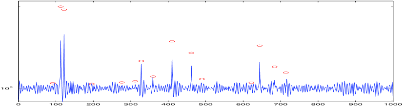
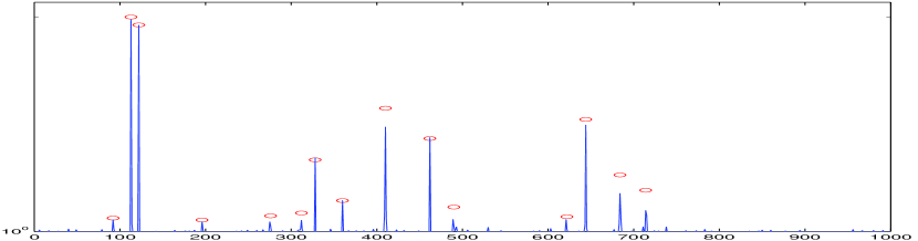
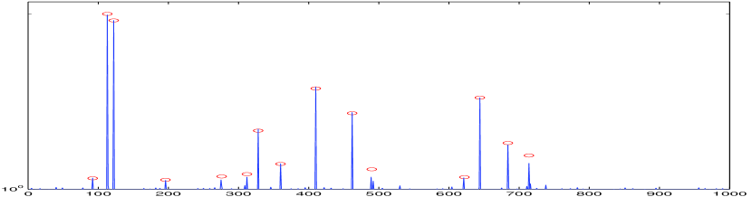
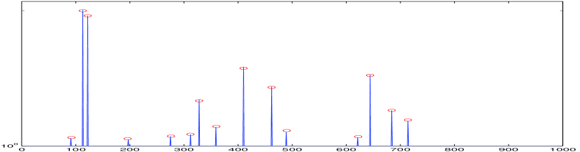
Figure 3: Deconvolution results with different priors: a) Gaussian  b) Gaussian truncated to positive axis  c) Generalized Gaussian. d) $-x\ln x$ entropic prior   e) $\ln x$ entropic or Gamma prior.

As it can be seen from these results , for this application, the Gaussian prior does not give satisfactory result, but in almost all the other cases the results are more satisfactory, because the corresponding priors are more in agreement with the nature of the unknown input signal.

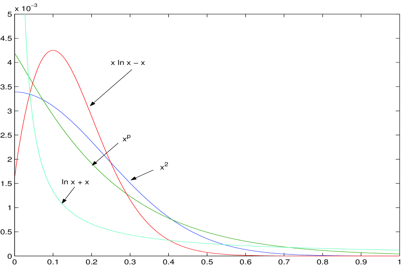
Figure 4: Plots of the different prior laws $p(x)\propto\exp\left[{-\lambda\phi(x)}\right]$: a) Truncated Gaussian   $\phi(x)=x^{2},\lambda=3$  b) Truncated generalized Gaussian   $\phi(x)=x^{p},\;p=1.1,\;\lambda=4$; c) Entropic $\phi(x)=x\ln x-x,\lambda=10$  d) Entropic $\phi(x)=\ln x+x,\lambda=0.1$.

The Gaussian prior (a) is not at all appropriate, Gaussian truncated to positive axis (b) is a better choice. The generalized Gaussian truncated to positive axis (c) and the $-x\ln x$ entropic priors (d) give also almost the same results than the truncated Gaussian case. The Gamma prior (e) seems to give slightly better result (less missing and less artifacts) than all the others. This can be explained if we compare the shape of all these priors shown in figure (4). The Gamma prior is sharper near to zero and has longer tail than other priors. It thus favorites signals with greater number of samples near to zero and still leaves the possibility to have very high amplitude pulses. However, we must be careful on this interpretation, because all these results depend also on the hyperparameter $\lambda$ whose value may be critical for this conclusion. In these experiments we used the same value for all cases. This brings us to the next open problem which is the determination of the hyperparameters.

5.2 Hyperparameter estimation

The Bayesian approach can be exactly applied when the direct (prior) probability laws $p({\mbox{\boldmath$y$}}|{\mbox{\boldmath$x$}},{\mbox{\boldmath$\phi$}}_{1})$ and $p({\mbox{\boldmath$x$}}|{\mbox{\boldmath$\phi$}}_{2})$ are assigned. Even, when we have chosen appropriate laws, still we have to determine their parameters ${\mbox{\boldmath$\phi$}}=[{\mbox{\boldmath$\phi$}}_{1},{\mbox{\boldmath$\phi$}}_{2}]$. This problem has been addressed by many authors and the subject is an active area in statistics. See Hall87 ; Hebert92 ; Johnson91 ; Titterington85 , Younes88 ; Younes89 ; Bouman94 ; Fessler93 ; Liang92 and also Fortier93 ; Djafari93a ; Djafari96b .

The Bayesian approach gives natural tools to handle this problem by considering ${\mbox{\boldmath$\phi$}}=({\mbox{\boldmath$\phi$}}_{1},{\mbox{\boldmath$\phi$}}_{2})$ as extra unknown parameters to infer on. We may then assign a prior law $p({\mbox{\boldmath$\phi$}})$ to them too. However, the way to do this is also still an open problem. We do not discuss it more in this paper. The readers are invited to see Kass94 for some extended discussions and references. When this step is done, we can again use the Bayesian approach and compute the joint posterior $p({\mbox{\boldmath$x$}},{\mbox{\boldmath$\phi$}}|{\mbox{\boldmath$y$}})$ from which we can follow three main directions:

– Joint MAP optimization: In this approach one tries to estimate both the hyperparameters and the unknown variables $x$ directly from the data by defining:

$$(\widehat{{\mbox{\boldmath$x$}}},\widehat{{\mbox{\boldmath$\phi$}}})=\mathop{\mbox{arg}\max}_{({\mbox{\boldmath$x$}},{\mbox{\boldmath$\phi$}})}\left\{{p({\mbox{\boldmath$x$}},{\mbox{\boldmath$\phi$}}|{\mbox{\boldmath$y$}})}\right\}\mbox{~{}where~{}}p({\mbox{\boldmath$x$}},{\mbox{\boldmath$\phi$}}|{\mbox{\boldmath$y$}})\propto p({\mbox{\boldmath$y$}}|{\mbox{\boldmath$x$}},{\mbox{\boldmath$\phi$}})\,p({\mbox{\boldmath$x$}}|{\mbox{\boldmath$\phi$}})\,p({\mbox{\boldmath$\phi$}})$$ (40)

and where $p({\mbox{\boldmath$\phi$}})$ is an appropriate prior law for $\phi$. Many authors used the non informative prior law for them.
– Marginalization: The main idea in this approach is to distinguish between the two sets of unknowns: a high dimensional vector $x$ representing in general a physical quantity and a low dimensional vector $\phi$ representing the parameters of its prior probability laws. This argument leads to estimate first the hyperparameters by marginalizing over the unknown variables $x$:

$$p({\mbox{\boldmath$\phi$}}|{\mbox{\boldmath$y$}})\propto p({\mbox{\boldmath$\phi$}})\,\int\kern-11.00008pt\int p({\mbox{\boldmath$y$}}|{\mbox{\boldmath$x$}},{\mbox{\boldmath$\phi$}})\,p({\mbox{\boldmath$x$}}|{\mbox{\boldmath$\phi$}}){\;\mbox{d}{\mbox{\boldmath$x$}}}$$ (41)

and then, using them in the estimation of the unknown variables $x$:

$$\widehat{{\mbox{\boldmath$\phi$}}}=\mathop{\mbox{arg}\max}_{{\mbox{\boldmath$\phi$}}}\left\{{p({\mbox{\boldmath$\phi$}}|{\mbox{\boldmath$y$}})}\right\}\longrightarrow\widehat{{\mbox{\boldmath$x$}}}=\mathop{\mbox{arg}\max}_{{\mbox{\boldmath$x$}}}\left\{{p({\mbox{\boldmath$x$}}|{\mbox{\boldmath$y$}},\widehat{{\mbox{\boldmath$\phi$}}})}\right\}.$$ (42)

Note also that when $p({\mbox{\boldmath$\phi$}})$ is choosed to be uniform, then $p({\mbox{\boldmath$\phi$}}|{\mbox{\boldmath$y$}})\propto p({\mbox{\boldmath$y$}}|{\mbox{\boldmath$\phi$}})$ which is the likelihood of the hyperparameters $\phi$ and the corresponding maximum likelihood (ML) estimate has all the good asymptotic properties which may not be the case for the joint MAP estimation. However, for practical applications with finite data we may not care too much about the asymptotic properties of these estimates.
– Nuisance parameters: In this approach the hyperparameters are considered as the nuisance parameters, so integrated out of $p({\mbox{\boldmath$x$}},{\mbox{\boldmath$\phi$}}|{\mbox{\boldmath$y$}})$ to obtain $p({\mbox{\boldmath$x$}}|{\mbox{\boldmath$y$}})$ and $x$ is estimated by

$$\widehat{{\mbox{\boldmath$x$}}}=\mathop{\mbox{arg}\max}_{{\mbox{\boldmath$x$}}}\left\{{p({\mbox{\boldmath$x$}}|{\mbox{\boldmath$y$}})}\right\}\mbox{~{}~{}where~{}~{}}p({\mbox{\boldmath$x$}}|{\mbox{\boldmath$y$}})=\int\kern-11.00008pt\int p({\mbox{\boldmath$y$}},{\mbox{\boldmath$x$}},{\mbox{\boldmath$\phi$}}){\;\mbox{d}{\mbox{\boldmath$\phi$}}}$$ (43)

– Joint Posterior Mean: Here, $x$ and $\phi$ are estimated as the posterior means:

$$\widehat{{\mbox{\boldmath$x$}}}=\mbox{E}\left\{{\mbox{\boldmath$x$}}|{\mbox{\boldmath$y$}}\right\}=\int\kern-11.00008pt\int{\mbox{\boldmath$x$}}\,p({\mbox{\boldmath$x$}}|{\mbox{\boldmath$y$}}){\;\mbox{d}{\mbox{\boldmath$x$}}}\mbox{~{}~{}and~{}~{}}\widehat{{\mbox{\boldmath$\phi$}}}=\mbox{E}\left\{{\mbox{\boldmath$\phi$}}|{\mbox{\boldmath$y$}}\right\}=\int\kern-11.00008pt\int{\mbox{\boldmath$\phi$}}\,p({\mbox{\boldmath$\phi$}}|{\mbox{\boldmath$y$}}){\;\mbox{d}{\mbox{\boldmath$\phi$}}}.$$ (44)

The main issue here is that, excepted the first approach, all the others need integrations for which, in general, there is not analytical expressions and their numerical computation cost may be very high. At the other hand, unfortunately, the estimation by the joint maximization has not the good asymptotic properties (when number of data goes to infinity) of the estimators obtained through the marginalization or expectation. However, in finite number of data, a comparison of their relative properties is still to be done. To see some more discussions and different possible implementations of these approaches see Djafari96b . We have also to mention that, we can always use the Markov Chain Monte Carlo (MCMC) techniques to generate samples from the joint posterior $p({\mbox{\boldmath$x$}},{\mbox{\boldmath$\phi$}}|{\mbox{\boldmath$y$}})$ and then compute the joint posterior means and corresponding variances. It seems that these techniques are growing up. However, I see two main limitations for their application on real data: their huge computational cost and the need for some discussions on the tools to control their convergences.

5.3 Myopic or blind inversion problems

Consider the deconvolution problems (1) or (2) and assume now that the psf $h(t)$ or $h(x,y)$ are partially known. For example, we know they have Gaussian shape, but the amplitude $a$ and the width $\sigma$ of the Gaussian are unknown. Noting by ${\mbox{\boldmath$\theta$}}=(a,\sigma)$ the problem then becomes the estimation of both $x$ and $\theta$ from ${\mbox{\boldmath$y$}}={\mbox{\boldmath$H$}}_{{\mbox{\boldmath$\theta$}}}{\mbox{\boldmath$x$}}+{\mbox{\boldmath$\epsilon$}}$. The case where we know only the support of the psf but not its shape can also be casted in the same way with ${\mbox{\boldmath$\theta$}}=[h(0),\ldots,h(p)]$

Before going more in details, we must note that, in general, the blind inversion problems are much harder than the simple inversion. Taking the deconvolution problem, we have seen in introduction that, the problem even when the psf is given is ill-posed. The blind deconvolution then is still more ill-posed, because here there are more fundamental under-determinations. For example, it is easy to see that, we can find an infinite number of pairs $(h,x)$ which result to the same convolution product $h*x$. This means that, to find satisfactory methods and algorithms for these problems need much more prior knowledge both on $x$ and on $h$, and in general, the inputs must have more structures (be rich in information content) to be able to obtain satisfactory results.

Conceptually however, the problem is identical to the estimation of hyperparameters in previous section and any of the four approaches presented there can be used. One may wish however to distinguish between these parameters of the system ${\mbox{\boldmath$\theta$}}=(a,\sigma)$ and those hyperparameters of the prior law model descriptions ${\mbox{\boldmath$\phi$}}=(\sigma_{\epsilon}^{2},\sigma_{x}^{2},\ldots)$. In that case, one can try to write down $p({\mbox{\boldmath$x$}},{\mbox{\boldmath$\theta$}},{\mbox{\boldmath$\phi$}}|{\mbox{\boldmath$y$}})$ and use one of the following:

– Joint MAP estimation of $x$, $\theta$ and $\phi$: $\displaystyle{(\widehat{{\mbox{\boldmath$x$}}},\widehat{{\mbox{\boldmath$\theta$}}},\widehat{{\mbox{\boldmath$\phi$}}})=\mathop{\mbox{arg}\max}_{({\mbox{\boldmath$x$}},{\mbox{\boldmath$\theta$}},{\mbox{\boldmath$\phi$}})}\left\{{p({\mbox{\boldmath$x$}},{\mbox{\boldmath$\theta$}},{\mbox{\boldmath$\phi$}}|{\mbox{\boldmath$y$}})}\right\}}$.
– Marginalize over $x$ and estimate $\theta$ and $\phi$ using: $\displaystyle{(\widehat{{\mbox{\boldmath$\theta$}}},\widehat{{\mbox{\boldmath$\phi$}}})=\mathop{\mbox{arg}\max}_{({\mbox{\boldmath$\theta$}},{\mbox{\boldmath$\phi$}})}\left\{{p({\mbox{\boldmath$\theta$}},{\mbox{\boldmath$\phi$}}|{\mbox{\boldmath$y$}})}\right\}}$ and then, estimate $x$ using: $\widehat{{\mbox{\boldmath$x$}}}=\mathop{\mbox{arg}\max}_{{\mbox{\boldmath$x$}}}\left\{{p({\mbox{\boldmath$x$}}|{\mbox{\boldmath$y$}},\widehat{{\mbox{\boldmath$\theta$}}},\widehat{{\mbox{\boldmath$\phi$}}})}\right\}$.
– Marginalize over $x$ and $\theta$ and estimate $\phi$ using: $\displaystyle{\widehat{{\mbox{\boldmath$\phi$}}}=\mathop{\mbox{arg}\max}_{{\mbox{\boldmath$\phi$}}}\left\{{p({\mbox{\boldmath$\phi$}}|{\mbox{\boldmath$y$}})}\right\},}$, then estimate $\theta$ using: $\widehat{{\mbox{\boldmath$\theta$}}}=\mathop{\mbox{arg}\max}_{{\mbox{\boldmath$\theta$}}}\left\{{p({\mbox{\boldmath$\theta$}}|{\mbox{\boldmath$y$}},\widehat{{\mbox{\boldmath$\phi$}}})}\right\}$ and finally, estimate $x$ using: $\widehat{{\mbox{\boldmath$x$}}}=\mathop{\mbox{arg}\max}_{{\mbox{\boldmath$x$}}}\left\{{p({\mbox{\boldmath$x$}}|{\mbox{\boldmath$y$}},\widehat{{\mbox{\boldmath$\theta$}}},\widehat{{\mbox{\boldmath$\phi$}}})}\right\}$.
– Joint Posterior Mean: Here, $x$, $\theta$ and $\phi$ are estimated through their respective posterior means: $\widehat{{\mbox{\boldmath$x$}}}=\mbox{E}\left\{{\mbox{\boldmath$x$}}|{\mbox{\boldmath$y$}}\right\}$, $\widehat{{\mbox{\boldmath$\theta$}}}=\mbox{E}\left\{{\mbox{\boldmath$\theta$}}|{\mbox{\boldmath$y$}}\right\}$ and $\widehat{{\mbox{\boldmath$\phi$}}}=\mbox{E}\left\{{\mbox{\boldmath$\phi$}}|{\mbox{\boldmath$y$}}\right\}$.

Here again, the joint optimization stays the simpler but we must be careful on interpretation of the results. For others, one can either use the Expectation-Maximization (EM) algorithms and/or MCMC sampling tools to approximately compute the necessary integration or expectation computations and overcome the computational cost issues.

6 Conclusions

In this paper I presented a synthetic overview of methods for inversion problems starting by deterministic data matching and regularization methods followed by a general presentation of the probabilistic methods such as error probability law matching and likelihood based and the information theory and maximum entropy based methods. Then, I focused on the Bayesian inference. I show that, as it concerns the maximum a posteriori estimation method, one can see easily the link with regularization methods. We discussed however the superiority of the Bayesian framework which gives naturally the necessary tools for inferring the uncertainty of the computed solution, for the estimation of the hyperparameters or for handling myopic and blind inversion problems. We saw also that probabilistic modeling of signal and images is more flexible for introduction of practical prior knowledge about them. Finally, we illustrated some of these discussions through a deconvolution example in mass spectrometry data processing.

References

- (1) M. Bertero, T. A. Poggio, and V. Torre, “Ill-posed problems in early vision,” Proceedings of the IEEE, 76, pp. 869–889, août 1988.
- (2) G. Demoment, “Image reconstruction and restoration: Overview of common estimation structure and problems,” IEEE Transactions on Acoustics, Speech and Signal Processing, assp-37, pp. 2024–2036, décembre 1989.
- (3) J. Skilling, “Theory of maximum entropy image reconstruction,” in Maximum Entropy and Bayesian Methods in Applied Statistics, Proc. of the Fourth Max. Ent. Workshop, J. H. Justice, ed., (Calgary), Cambridge Univ. Presse, 1984.
- (4) R. J. Hanson, “A numerical method for solving fredholm integral equations of the first kind using singular values,” SIAM Journal of Numerical Analysis, 8, pp. 616–622, 1971.
- (5) J. Idier, A. Mohammad-Djafari, and G. Demoment, “Regularization methods and inverse problems: an information theory standpoint,” in 2nd International Conference on Inverse Problems in Engineering, (Le Croisic), pp. 321–328, juin 1996.
- (6) D. M. Titterington, “Common structure of smoothing techniques in statistics,” International Statistical Review, 53, (2), pp. 141–170, 1985.
- (7) G. H. Golub, M. Heath, and G. Wahba, “Generalized cross-validation as a method for choosing a good ridge parameter,” Technometrics, 21, pp. 215–223, mai 1979.
- (8) N. Fortier, G. Demoment, and Y. Goussard, “gcv and ml methods of determining parameters in image restoration by regularization: Fast computation in the spatial domain and experimental comparison,” Journal of Visual Communication and Image Representation, 4, pp. 157–170, juin 1993.
- (9) G. Le Besnerais, J.-F. Bercher, and G. Demoment, “A new look at entropy for solving linear inverse problems,” IEEE Transactions on Information Theory, 45, pp. 1565–1578, juillet 1999.
- (10) A. Mohammad-Djafari and J. Idier, “Scale invariant Bayesian estimators for linear inverse problems,” in Proc. of the First ISBA meeting, (San Francisco, ca), août 1993.
- (11) S. Brette, J. Idier, and A. Mohammad-Djafari, Scale invariant Markov models for Bayesian inversion of linear inverse problems, pp. 199–212. Maximum Entropy and Bayesian Methods, Kluwer Academic Publ., Cambridge, uk, J. Skilling & S. Sibusi ed., 1994.
- (12) S. Brette, J. Idier, and A. Mohammad-Djafari, “Scale invariant Markov models for linear inverse problems,” in Proc. of the Section on Bayesian Statistical Sciences, (Alicante,), pp. 266–270, American Statistical Association, 1994.
- (13) S. Brette, J. Idier, and A. Mohammad-Djafari, “Scale invariant Bayesian estimator for inversion of noisy linear system,” Fifth Valencia Int. Meeting on Bayesian Statistics, juin 1994.
- (14) F. Champagnat, Y. Goussard, and J. Idier, “Unsupervised deconvolution of sparse spike trains using stochastic approximation,” IEEE Transactions on Signal Processing, 44, pp. 2988–2998, décembre 1996.
- (15) P. Hall and D. M. Titterington, “Common structure of techniques for choosing smoothing parameter in regression problems,” Journal of the Royal Statistical Society B, 49, (2), pp. 184–198, 1987.
- (16) T. J. Hebert and R. Leahy, “Statistic-based map image reconstruction from poisson data using Gibbs prior,” IEEE Transactions on Signal Processing, 40, pp. 2290–2303, septembre 1992.
- (17) V. Johnson, W. Wong, X. Hu, and C.-T. Chen, “Image restoration using Gibbs priors: Boundary modeling, treatement of blurring, and selection of hyperparameter,” IEEE Transactions on Pattern Analysis and Machine Intelligence, pami-13, (5), pp. 413–425, 1984.
- (18) L. Younès, “Estimation and annealing for Gibbsian fields,” Annales de l’institut Henri Poincaré, 24, pp. 269–294, février 1988.
- (19) L. Younes, “Parametric inference for imperfectly observed Gibbsian fields,” Prob. Th. Rel. Fields, 82, pp. 625–645, 1989.
- (20) C. A. Bouman and K. D. Sauer, “Maximum likelihood scale estimation for a class of Markov random fields penalty for image regularization,” in Proceedings of the International Conference on Acoustic, Speech and Signal Processing, vol. V, pp. 537–540, 1994.
- (21) J. A. Fessler and A. O. Hero, “Complete data spaces and generalized em algorithms,” in Proceedings of the International Conference on Acoustic, Speech and Signal Processing, (Minneapolis, Minnesota), pp. IV 1–4, 1993.
- (22) K.-Y. Liang and D. Tsou, “Empirical Bayes and conditional inference with many nuisance parameters,” Biometrika, 79, (2), pp. 261–270, 1992.
- (23) A. Mohammad-Djafari, “On the estimation of hyperparameters in Bayesian approach of solving inverse problems,” in Proceedings of the International Conference on Acoustic, Speech and Signal Processing, (Minneapolis, mn), pp. 567–571, ieee, avril 1993.
- (24) A. Mohammad-Djafari, A full Bayesian approach for inverse problems, pp. 135–143. Kluwer Academic Publishers, Santa Fe, nm, K. Hanson and R.N. Silver ed., 1996.
- (25) R. E. Kass and L. Wasserman, “Formal rules for selecting prior distributions: A review and annotated bibliography,” technical report no. 583, Department of Statistics, Carnegie Mellon University, Submitted to J. of American Statistical Association, 1994.