Control of Switched Networks via Quantum Methods

Abstract

We illustrate a technique for specifying piecewise constant controls for classes of switched electrical networks, typically used in converting power in a dc-dc converter. This procedure makes use of decompositions of $SU(2)$ to obtain controls that are piecewise constant and can be constrained to be bang-bang with values $0$ or $1$. Complete results are presented for a third order network first. An example, which shows that the basic strategy is viable for fourth order circuits, is also given. The former evolves on $SO(3)$, while the latter evolves on $SO(4)$. Since the former group is intimately related to $SU(2)$ while the latter is related to $SU(2)\times SU(2)$, the methodology of this paper uses factorizations of $SU(2)$. The systems in this paper are single input systems with drift. In this paper, no approximations or other artifices are used to remove the drift. Instead, the drift is important in the determination of the controls. Periodicity arguments are rarely used.

Keywords: bang-bang controls, piecewise constant controls, Lie group, bilinear system, switched electrical network.

1
Introduction

In this paper the problem of explicit control of a class of switched electrical, lossless networks is considered. Specifically, it is shown how to determine explicitly piecewise controls, which can be constrained to take only the values $1$ or $0$, to achieve state transfers. Complete results are obtained for a third order lossless network, which has been studied before in [11], [2], [7]. The thesis, [11], provides the model and assesses the controllability of the network. The paper, [7], uses averaging to provide periodic controls for approximate state preparation. The same reference also emphasizes the desirability of finding bang-bang controls (with values $1$ or $0$), since this mode of control is closer to physical reality. In this paper a constructive protocol for precisely such a bang-bang control is provided. A fourth order network is also studied and preliminary results on certain explicit state transfers via bang-bang controls are provided.

The energy conservation of the networks implies that they evolve on $SO(3)$ (respectively $SO(4)$). For the third order network, the problem of bang-bang controls is susceptible to Euler factorizations (though non-Euler factorizations are also pertinent). However for constructiveness, explicit formulae, providing the Euler angles as expressions in the entries of the target state in $SO(3)$, have to be supplied. To the best of our knowledge such explicit formulae are missing in the literature, especially when the two generators of $so(3)$ (the Lie algebra of $SO(3)$), desired in the factorization, are the ones relevant to the model. It is worth emphasizing that the desired state in $SO(3)$ does not already come specified with its Euler angles. Rather, it is described by the nine real entries which constitute this matrix. Similar issues (with the technicalities compounded) present themselves for the fourth order network. It is primarily for this reason that the methodology of this paper uses a passage to an associated system evolving on $SU(2)$ (respectively $SU(2)\times SU(2)$). For the system associated to the third order network it turns out that Euler angles for $SU(2)$, when the two generators are $i\sigma_{x}$ and $i\sigma_{y}$, are needed. These are easier than the corresponding $SO(3)$ angles to calculate because of two reasons: i) first, $SU(2)$ matrices are $2\times 2$ (the special unitarity mitigates the fact that the entries are complex) and thus, the matrix manipulations (which are inevitable if explicit formulae are required) are easier; and ii) $SU(2)$ matrices admit the following representation (the Cayley-Klein representation):

$$S=S\left(\alpha,\zeta,\mu\right)=\left(\begin{array}[]{cc}e^{i\zeta}\cos\alpha&e^{i\mu}\sin\alpha\\ e^{i\left(\pi-\mu\right)}\sin\alpha&e^{-i\zeta}\cos\alpha\end{array}\right).$$ (1)

One such representation is nothing more than the entries written in polar coordinates. The advantage of (1) is that the condition $SS^{\ast}=S^{\ast}S=I,$ $\det\left(S\right)=1$, is already incorporated. In contrast to $SO(3),$ side conditions need not be stipulated. The attendant formulae, for even the $SU(2)$ Euler angles, are messier if Cartesian coordinates were to be used (in our opinion, this is one of the reasons why explicit formulae for $\left(x,y\right)$ Euler angles for $SO(3)$ are not available - there is no polar representation for real numbers). Furthermore, representing the columns of an $SO(3)$ matrix in spherical coordinates is equally unilluminating. In addition, for finding non-Euler factorizations, $SU(2)$ is easier to work with.

The differences between the third order network and the fourth order network examples are primarily twofold: i) for the fourth order network, factorizations of $SU(2)$, different from $\sigma_{x},\sigma_{y}$ Euler angles, are needed. Indeed, the required factorizations are not of the Euler type. Such factorizations are easier to find when working with $SU(2).$ ii) More importantly, the fourth order network problem amounts to the difficult question of constructive control of two systems with a single control. Due to the latter problem our results for the fourth order circuit are, pending further investigation, applicable under certain conditions on the circuit. Specifically, the transfers are achieved if any one of a set of relations between the constants of the circuits are satisfied. In part, these relations are a by-product of the specific choice of factorizations used. It should be possible to achieve these relations in practice, since they are only restrictions on the capacitors and inductors in the circuit. Work is ongoing to enlarge the class of state transfers and also to eliminate the restrictions on the constants. These preliminary results are, to the best of our knowledge, the first instances of constructive controllability for single input systems with drift evolving on $SO(4).$ It is our opinion that, regardless of the specific model or the control technique, the most elegant manner to control a system evolving on $SO(4)$ would indeed be to pass to an associated system on $SU(2)\times SU(2)$. Readers who are skeptical should first attempt to calculate the exponential of an $so(4)$ matrix without any usage of $SU(2)$ whatsoever. At a bare minimum manipulation of $4\times 4$ matrices is required, whereas passage to $SU\left(2\right)\times SU(2)$ obviates all matrix manipulations. More importantly, finding $e^{A},$ $A\in so(4),$ via eigenvalues etc., occludes the structure of $A$ in $e^{A}.$ This structure is relevant to the problem.

Thus, the close relation between $SU(2)$, $SO(3)$ and $SO(4)$ is used for the network systems. The group, $SU(2)$, plays a prominent role in the control of many quantum systems (atoms and molecules, Cooper pairs, spin systems, photons and excitons). This explains the title of the paper. The rich algebraic structure of the Pauli matrices makes the deduction of the formulae easier than on the orthogonal groups. However, once a formula has been found on $SU(2)$ - whether it be for an exponential or bang-bang controls etc., - it can be transferred easily to the orthogonal group. This is the rationale behind our method.

Systems such as dc-dc switchmode power converters, in which switched electrical networks have a significant part, can be implemented in communication and data handling systems, portable battery-operated equipment and other applications. Thus, the results of this paper have useful consequences for these applications. Other strategies for controlling switched electrical networks use state-space averaging. Leonard and Krishnaprasad [7] transform these systems into drift free systems and then apply averaging theory on Lie groups to specify small amplitude, periodic, open-loop controls for approximate state transfers. The approach of Sira-Ramirez [10], based on variable structure systems theory and sliding regimes, provides feedback controls for switched electrical networks. In contrast, the method in this paper obtains piecewise constant controls which further can be taken to be 0 or 1, corresponding to the position of the switch. From the results of Jurdjevic and Sussmann [6] it is known that bang-bang controls with values of 0 and 1 can be used to prepare any target. Thus, the paper provides constructive illustrations of the work in [6]. It is emphasized that the approach taken in this paper does not resort to techniques for driftless systems by either i.) removing the drift via approximations or other methods which work only in fortuitous situations or ii.) by making use of periodicity. Arguments relying on periodicity are invalid in general [8] and can lead to expensive controls even when valid. In this paper the only time periodicity is used is to rewrite free evolution terms with negative drift coefficients as free evolution terms with positive drift coefficients.

The balance of this paper is organized as follows. In section 2, the relations between the unitary and orthogonal groups are reviewed. In the next section, the precise model for the $SO(3)$ network is presented. Controls for this system are obtained in section 4. This section also contains the relevant formulae for the desired Euler angles. These are used to provide, first, piecewise constant controls and then bang-bang controls. The fifth section provides an illustration of the techniques for the fourth order network. The final section offers some conclusions.

2 $SU(2)$, $SO(3)$ and $SO(4)$

The Lie algebras $su(2)=\{V\in\mathbb{C}^{2\times 2}\mid V^{\ast}=-V\}$ and $so(3)=\{W\in\mathbb{R}^{3\times 3}\mid W^{T}=-W\}$ are isomorphic via the following explicit isomorphism, [1]:

$$\psi\left[-\frac{i}{2}\left(a\sigma_{x}+b\sigma_{y}+c\sigma_{z}\right)\right]=\left(\begin{array}[]{ccc}0&-c&b\\ c&0&-a\\ -b&a&0\end{array}\right),$$ (2)

with

$$\sigma_{x}=\left(\begin{array}[]{cc}0&1\\ 1&0\end{array}\right),\ \sigma_{y}=\left(\begin{array}[]{cc}0&-i\\ i&0\end{array}\right)\text{ and }\sigma_{z}=\left(\begin{array}[]{cc}1&0\\ 0&-1\end{array}\right).$$

Similarly, there is a group homomorphism $\phi:SU(2)\rightarrow SO(3),$ [1], obtained by considering the linear (vector space) map, $R_{U}:su(2)\rightarrow su(2)$, which for a fixed $U\in SU(2)$ is given by $R_{U}(A)=UAU^{\ast}$. Identifying $su(2)$ with $R^{3}$, it can be shown that $R_{U}\in SO(3)$. The group homomorphism, $\phi,$ just associates $U$ to $R_{U}$. Finally, it can be shown, via a direct calculation using the Rodrigues’ formula, that $\phi(e^{K})=e^{\psi(K)}$.

The groups $SO(4)$ and $SU(2)$ are related as follows. First, identifying the quaternions with $R^{4}$ via $e_{1}=1,\ e_{2}=i,\ e_{3}=j,\ e_{4}=k$, leads to the following association, $I$, between a pair of unit quaternions, $p,q$ and a linear map from $R^{4}$ to $R^{4},$ [1]:

$$I(p,q)=\text{{the linear map}, }x\rightarrow pxq^{-1}.$$

It can be shown that $I(p,q)$ is an element of $SO(4)$. Further, it is well known, [1], that the group of unit quaternions is explicitly isomorphic to $SU(2)$. This then leads to a group homomorphism, $\tilde{\phi}:SU(2)\times SU(2)\rightarrow SO(4)$. It can be shown, via a direct calculation, that there is an associated Lie algebra isomorphism, $\tilde{\psi}:su(2)\times su(2)\rightarrow so(4)$, which satisfies $\tilde{\phi}(e^{K_{1}},e^{K_{2}})=e^{\tilde{\psi}\left(K_{1}\times K_{2}\right)},$ for any $K_{1}\times K_{2}$ in $su(2)\times su(2)$. $\tilde{\psi}$ is given by

$$\tilde{\psi}\left(K_{1}\times K_{2}\right)=\left(\begin{array}[]{cccc}0&-a_{1}&-a_{2}&-a_{3}\\ a_{1}&0&-b_{3}&b_{2}\\ a_{2}&b_{3}&0&-b_{1}\\ a_{3}&-b_{2}&b_{1}&0\end{array}\right),$$ (3)

where

$$K_{1}=\left(\begin{array}[]{cc}\frac{i}{2}\left(a_{1}+b_{1}\right)&\frac{1}{2}\left[\left(a_{2}+b_{2}\right)+i\left(a_{3}+b_{3}\right)\right]\\ \frac{1}{2}\left[-\left(a_{2}+b_{2}\right)+i\left(a_{3}+b_{3}\right)\right]&-\frac{i}{2}\left(a_{1}+b_{1}\right)\end{array}\right)$$ (4)

and

$$K_{2}=\left(\begin{array}[]{cc}\frac{i}{2}\left(b_{1}-a_{1}\right)&\frac{1}{2}\left[\left(b_{2}-a_{2}\right)+i\left(b_{3}-a_{3}\right)\right]\\ \frac{1}{2}\left[-\left(b_{2}-a_{2}\right)+i\left(b_{3}-a_{3}\right)\right]&-\frac{i}{2}\left(b_{1}-a_{1}\right)\end{array}\right).$$ (5)

Thus, given a system $\dot{V}=\tilde{A}V+\tilde{B}Vu(t),$ $V\in SO(3)$, one can associate a system, $\dot{U}=AU+BUu(t),$ $U\in SU(2)$, where $A=\psi^{-1}(\tilde{A})$ and $B=\psi^{-1}(\tilde{B}),$ to it. Now preparing a target, $S$ in $SO(3)$ with piecewise constant controls amounts to factoring $S$ as $\Pi_{k=1}^{Q}e^{(a_{k}\tilde{A}+b_{k}\tilde{B})}$, with $a_{k}>0$, if $b_{k}\neq 0$. The condition, $b_{k}$ is either $0$ or $b_{k}=a_{k}$, is equivalent to preparing $S$ with controls only taking values $1$ or $0$. As mentioned in the introduction, obtaining such factorizations explicitly is easier for $SU(2)$. Hence, we work with the second system and factorize any matrix $T$ in $SU(2)$, such that $\phi(T)=S$, as $T=\prod_{k=1}^{Q}e^{(a_{k}A+b_{k}B)}$ with either $a_{k}>0$, if $b_{k}\neq 0$ etc. Recapitulating the preparation of a target $S$ in $SO(3)$ by associating it to a target $T$ in $SU(2),$

$$S=\phi\left(T\right)=\phi\left(\prod_{k=1}^{Q}e^{a_{k}A+b_{k}B}\right),$$ (6)

because $\phi$ is a homomorphism this gives

$$S=\prod_{k=1}^{Q}\phi\left(e^{a_{k}A+b_{k}B}\right),$$ (7)

and since $\phi(e^{K})=e^{\psi(K)},$

$$S=\prod_{k=1}^{Q}e^{a_{k}\tilde{A}+b_{k}\tilde{B}}.$$ (8)

Therefore the same controls that prepare $T$ also prepare $S.$ The corresponding control values are, of course, $\frac{b_{k}}{a_{k}}$.

Likewise, given a system $\dot{V}=\tilde{A}V+\tilde{B}Vu(t),$ $V\in SO(4)$, two systems controlled by a single control $\mathbf{u}\left(t\right)$, are associated to it via, $\dot{U_{1}}=A_{1}U_{1}+B_{1}U_{1}u(t),$ $U_{1}\in SU(2)$ and $\dot{U_{2}}=A_{2}U_{2}+B_{2}U_{2}u(t),$ $U_{2}\in SU(2)$. Here, $(A_{1},A_{2})=\tilde{\psi}^{-1}(\tilde{A})$ and $(B_{1},B_{2})=\tilde{\psi}^{-1}(\tilde{B})$. Given a target, $S\in SO(4)$, we prepare any $(T_{1},T_{2})$ such that $\tilde{\phi}(T_{1},T_{2})=S$. Usage of piecewise constant controls means that both the $T_{i}$ have to be factorized as $T_{i}=\Pi_{k=1}^{Q}e^{(a_{k}A_{i}+b_{k}B_{i})}$, with the same $Q$ and same $a_{k}$ and $b_{k}$ for all $k=1,\ldots,Q$. The usual stipulations, $a_{k}>0$ if $b_{k}\neq 0$ etc., apply here too.

Remark 1: It is well known, [1], that the kernel of $\phi$ is $\left\{+I_{2},-I_{2}\right\}$ and that the kernel of $\tilde{\phi}$ is $\left\{\left(I_{2},I_{2}\right),\left(-I_{2},-I_{2}\right)\right\}.$ In this paper we do not make systematic use of this extra degree of freedom.

3 The Third Order Network

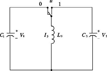
Figure 1: Third Order Switched Network

In this section, a switched electrical network with three circuit elements and no external constant power sources is considered. The switched electrical network examined here is identical to the one used by Leonard, Krishnaprasad and Wood [7], [11]. This network consists of two capacitors $C_{1}$ and $C_{2}$ with corresponding voltages $V_{1}$ and $V_{2}$ (see Figure 1). These capacitors are connected by a switch and an inductor $L_{3}$ with current $I_{3}$. The position of the switch connected to a control takes only the values of $0$ or $1.$ The control objective is to transfer energy from $C_{1}$ to $C_{2}$ by means of the inductor. Such systems, in the absence of external loads, can be modeled [7] by defining the network state vector $\mathbf{x}=\left(x_{1},x_{2},x_{3}\right)^{T}$ as $x_{1}=\sqrt{C_{1}}V_{1}$, $x_{2}=\sqrt{C_{2}}V_{2}$, and $x_{3}=\sqrt{L_{3}}I_{3}$. Let $\omega_{1}=1/\sqrt{C_{1}L_{3}}$ and $\omega_{2}=1/\sqrt{C_{2}L_{3}}$. Then the system is

$$\frac{d}{dt}\mathbf{x}=\left(\begin{array}[]{ccc}0&0&\omega_{1}\left(1-u\right)\\ 0&0&\omega_{2}u\\ -\omega_{1}\left(1-u\right)&-\omega_{2}u&0\end{array}\right)x=\left(\tilde{A}+\tilde{B}u\right)\mathbf{x.}$$ (9)

If the control takes a constant value $u$ for a time $t$, the state of the system can be written as

$$\mathbf{x}\left(t\right)=e^{\left(\tilde{A}+\tilde{B}u\right)t}\mathbf{x}\left(0\right).$$ (10)

The system on $SU\left(2\right)$ associated to the system on $SO\left(3\right),$ from section 2, is

$$\frac{d}{dt}U=\left(-\frac{i}{2}\omega_{1}\sigma_{y}+\frac{i}{2}\left(\omega_{1}\sigma_{y}+\omega_{2}\sigma_{x}\right)u\right)U\mathbf{.}$$ (11)

4 Quantum Control Techniques

Preparing the final state, $\mathbf{x}_{f},$ is equivalent to the preparation of one of an infinite family of $SO(3)$ matrices such that $\mathbf{x}_{f}=S\mathbf{x}\left(0\right).$ This, in turn, defines a family of targets in $SU(2)$ that can be associated with each such $S.$ Each target $S\in SO(3)$ corresponds to two targets in $SU(2).$ Preparing either of these two targets amounts to preparing $S.$

A target $T\in$ $SU(2),$ can be written as

$$T=\exp\left[-\frac{i}{2}\left(a\sigma_{x}+b\sigma_{y}+c\sigma_{z}\right)\right],$$ (12)

where $a,b,c\in\mathbb{R}.$ Let $\lambda=\frac{1}{2}\sqrt{a^{2}+b^{2}+c^{2}}$, $s=-\frac{i}{2}\left(a\sigma_{x}+b\sigma_{y}+c\sigma_{z}\right)$ and $\mathbf{p}=\left(\begin{array}[]{ccc}a&b&c\end{array}\right)^{T}.$ An expression for the Lie group homomorphism, $\phi,$ described in section 2 is obtained from Rodrigues’ formula [5],

$$\exp\left[\psi\left(s\right)\right]=I\cos 2\lambda+\frac{\sin 2\lambda}{2\lambda}\psi\left(s\right)+\frac{1-\cos 2\lambda}{4\lambda^{2}}\mathbf{pp}^{T},$$ (13)

by using equation (2) and the fact that $\phi\left(T\right)=\exp\left[\psi\left(s\right)\right].$ Now the problem of finding controls to drive the switched network on $SO(3)$ from $\mathbf{x}\left(0\right)$ to $\mathbf{x}_{f}$ is converted to finding controls that prepare $T\in SU(2).$ This is accomplished by using an appropriate decomposition of $T.$

4.1 Decompositions of a target in SU(2)

The general problem of preparing targets in $SU(2)$ was considered in [8]. In that work the theory requires that the drift and control matrices $A$ and $B$ be orthonormal. Orthonormality of $A$ and $B$ can be achieved by preliminary controls. The use of preliminary controls precludes the construction of bang-bang controls. Since preliminary orthonormalization of the matrices $A$ and $B$ is not used here, the results do not follow directly from [8]. However, the general framework of that paper is helpful in this work.

Consider the general problem of preparing a target for the system (11) in $SU(2)$. The decompositions of elements of $SU(2)$ considered in this paper are based on the fact that $A$ and $B$ in (11) are linear combinations of $i\sigma_{x}$ and $i\sigma_{y}.$ By writing the entries of $T$ in the Cayley-Klein representation (1), various decompositions can be obtained. We describe three of these factorizations, one of which is used for general piecewise constant controls and the other two for bang-bang controls. First as shown in [8], matrices in $SU(2)$ may be decomposed into the following form:

$$T\left(\alpha,\zeta,\mu\right)=e^{ip\sigma_{z}}V\left(\gamma\right)e^{i\left(\zeta-p\right)\sigma_{z}},$$ (14)

for any $p\in\mathbb{R}$ and

$$V\left(\gamma\right)=\exp\left(\begin{array}[]{cc}0&i\gamma\\ i\bar{\gamma}&0\end{array}\right)=\exp\left[\left(-\textnormal{Im}\gamma\right)i\sigma_{y}+\left(\textnormal{Re}\gamma\right)i\sigma_{x}\right]$$ (15)

for $\gamma\in\mathbb{C}.$ In equation (14), $\gamma=\alpha\exp i\left(\zeta+\mu-2p-\frac{\pi}{2}\right)$ and $p$ can be chosen so that $V\left(\gamma\right)$ is a free evolution factor. For the switched electrical network considered in this paper, the first and third factors of equation (14) have a useful decomposition. In [9], it was proved that the exponential of the third Pauli matrix can be expressed as a product of two factors

$$e^{iL\sigma_{z}}=V\left(\gamma_{1}\right)V\left(\gamma_{2}\right),$$ (16)

where $L\in\mathbb{R}$. Thus it follows from equation (14) that $T=\prod_{k=1}^{Q}V\left(\gamma_{k}\right),$ where $1\leq Q\leq 5.$ In (16), let $\gamma_{k}=\frac{\pi}{2}e^{i\theta_{k}},$ $k=1,2,$ then it holds that $L=\theta_{1}-\theta_{2}+\pi.$ Since $L$ can be taken as an element of $[0,2\pi),$ it follows that $\left|L-\pi\right|<\pi,\ L\neq 0.$ Thus for $L\neq 0,$ $\gamma_{1}$ and $\gamma_{2}$ can be chosen so that $\left|\theta_{1}-\theta_{2}\right|<\pi.$ This means that $\gamma_{1}$ and $\gamma_{2}$ may be selected to lie any open half-plane. In other words, one can ensure that $a_{k}>0,$ $\forall k,$ as

$$V\left(\gamma_{k}\right)=\exp\left[b_{k}\frac{\omega_{2}}{2}i\sigma_{x}+\left(b_{k}-a_{k}\right)\frac{\omega_{1}}{2}i\sigma_{y}\right].$$ (17)

It follows that the half-plane of interest is $\textnormal{Im}\gamma_{k}>-\frac{\omega_{1}}{\omega_{2}}\textnormal{Re}\gamma_{k}.$ This decomposition of the target in $SU(2)$ provides piecewise constant controls with no further restrictions.

Remark 2: The utility of the decomposition (16) is the following. Together with equation (14) it provides a factorization of any $T$ in $SU\left(2\right)$ of the type given by equation (6), with generally lower values of $\sqrt{a_{k}^{2}+b_{k}^{2}}$ for each $k,$ than would a factorization provided by the Euler parametrization (eqtns (19)-(22) below). This can be seen by viewing each factor in both of these decompositions as a matrix, $V\left(\gamma\right)$ (cf. eqtn (15)).

The complex numbers, $\gamma,$ in the factorization provided by equation (16) each have a radial coordinate at most $\frac{\pi}{2},$ whereas the radial coordinates due to Euler factorizations could be as high as $2\pi.$ This causes the former factorization to yield, generally, lower values for (individual and cumulative) $\sqrt{a_{k}^{2}+b_{k}^{2}}.$ Since $a_{k}$ represents the duration and $b_{k}$ the power (=duration$\times$amplitude) of the $k$th pulse, this suggests that equation (16) is preferable for the simultaneous minimization of these two competing constraints, as long as it is reasonable to use any piecewise constant control.

Next consider bang-bang controls. For free evolution, $u_{k}=0,$ $b_{k}=0$ and from equation (17), $V\left(\gamma_{k}\right)=\exp\left(-a_{k}\frac{\omega_{1}}{2}i\sigma_{y}\right),$ or in other words, $\theta_{k}=\frac{\pi}{2}.$ When $u_{k}=1,$ this means that $a_{k}=b_{k},$ so that $V\left(\gamma_{k}\right)=\exp\left(b_{k}\frac{\omega_{2}}{2}i\sigma_{x}\right)$ which corresponds to the phase $\theta_{k}=0.$ These facts lead to the consideration of the following decomposition of the exponential of the third Pauli matrix:

$$e^{iL\sigma_{z}}=e^{-i\frac{7\pi}{4}\sigma_{y}}e^{iL\sigma_{x}}e^{-i\frac{\pi}{4}\sigma_{y}}.$$ (18)

The first and third factors of equation (18) are free evolution and the second factor is obtained with a control pulse of $1.$ In each factor of (18) the drift coefficient is a positive number. With this decomposition the target $T$ from equation (14), with $p$ chosen so that $V\left(\gamma\right)$ is a free evolution factor, is prepared by at most seven factors of which at most two are control pulses. Now we consider another decomposition of $T$ from which $T$ is prepared by at most three factors.

A different bang-bang protocol is obtained by the following. It is shown in [3] that the target $T$ can be expressed as

$$T\left(\alpha,\zeta,\mu\right)=e^{iD\sigma_{x}}e^{iE\sigma_{y}}e^{iF\sigma_{x}},$$ (19)

where $D$, $E$ and $F$ are solutions to the relations

$$\cos(E) = \pm\sqrt{\cos^{2}\zeta\cos^{2}\alpha+\sin^{2}\mu\sin^{2}\alpha}$$ (20)

$$\sin(D-F) = \pm\frac{\sin\zeta\cos\alpha}{\sqrt{\sin^{2}\zeta\cos^{2}\alpha+\cos^{2}\mu\sin^{2}\alpha}}$$ (21)

$$\sin(D+F) = \pm\frac{\sin\mu\sin\alpha}{\sqrt{\cos^{2}\zeta\cos^{2}\alpha+\sin^{2}\mu\sin^{2}\alpha}}.$$ (22)

Remark 3: The expressions for the Euler angles given by equations (20)-(22) were obtained by an explicit matrix calculation. Indeed, it is known that an Euler angle factorization, with factors that are exponentials of $i\sigma_{z}$ and $i\sigma_{y},$ exists with a maximum of three factors. The orthogonality of the pairs $\left(i\sigma_{z},i\sigma_{y}\right)$ and $\left(i\sigma_{x},i\sigma_{y}\right)$ suggests an obvious Lie algebra isomorphism of $su\left(2\right)$ with itself. This suggests that it should be possible to find a factorization of the type in equation (19). This matrix calculation is facilitated by an explicit expression for the exponential of an $su\left(2\right)$ matrix (which, incidently, is easier to manipulate than the corresponding $so\left(3\right)$ expression). Even though there is  a natural geometric equivalence between the pairs of generators of $su\left(2\right),$ $\left(i\sigma_{z},i\sigma_{y}\right)$ and $\left(i\sigma_{x},i\sigma_{y}\right),$ the expressions for the Euler angles are not simple consequences of one another. It is routine to show that the $\left(i\sigma_{z},i\sigma_{y}\right)$ Euler angles are linear in the Cayley-Klein coordinates, whereas, equations (20)-(22) demonstrate that the $\left(i\sigma_{x},i\sigma_{y}\right)$ Euler angles involve transcendental functions.

In the decomposition of $T$  in equation (19) the second factor is free evolution and control pulses of $1$ are used to obtain the first and third factors. This decomposition of $T$ prepares the target with at most three factors with no more than two control pulses. In summary, we have:

Algorithm 1

Piecewise constant controls.

1. Given an initial state $\mathbf{x}(0)$ and a final state $\mathbf{x}_{f},$ choose the numbers $a,b,$ and $c$ in equation (13) so that the target on $SO(3),$ $S=\exp\left[\psi\left(s\right)\right],$ satisfies $\mathbf{x}_{f}=S\mathbf{x}\left(0\right).$

2. Write the entries of $S$ in polar coordinates as in equation (1).

3. Choose $p$ in equation (14) so that $V\left(\gamma\right)$ is a free evolution factor.

4. For each of the first and third factors of equation (14) use the decomposition in equation (16). Select the phases of $\gamma_{1}=\frac{\pi}{2}e^{i\theta_{1}}$ and $\gamma_{2}=\frac{\pi}{2}e^{i\theta_{2}}$ in equation (16) so that $L=\theta_{1}-\theta_{2}+\pi$ and the drift coefficients are positive numbers.

Algorithm 2

Bang-bang controls I

Steps one through three are the same as for piecewise constant controls.

Step four: For each of the first and third factors of equation (14) use the decomposition in equation (18).

Algorithm 3

Bang-bang controls II

Steps one and two are the same as for piecewise constant controls.

Step three: Solve for $D$, $E$ and $F$ in the decomposition of $T$ given by equation (19).

4.2 Example

For the switched network in Figure 1, if $C_{1}=0.1,$ $C_{2}=0.2$ and $L_{3}=0.5,$ then $A=-\sqrt{5}i\sigma_{y}$ and $B=\frac{i}{2}\left(2\sqrt{5}\sigma_{y}+\sqrt{10}\sigma_{x}\right).$ Suppose the initial state vector $\mathbf{x}(0)=(1,0,0)^{T}$ and the final state vector $\mathbf{x}_{f}=(0,-1,0)^{T}.$ Intermediate points for the system to traverse may be specified such as $\mathbf{x}(t1)=(1/\sqrt{2},0,-1/\sqrt{2})^{T}$ for the first intermediate point and $\mathbf{x}(t2)=(0,-1/\sqrt{2},-1/\sqrt{2})^{T}$ for the second intermediate point [7]. Suppose that it is desired for the system to pass through the intermediate points $\mathbf{x}\left(t1\right)$ and $\mathbf{x}(t2).$ Then three targets $T_{1}$, $T_{2}$ and $T_{3}$ in $SU(2)$ must be prepared so that $\mathbf{x}\left(t1\right)=\phi\left(T_{1}\right)\mathbf{x}(0)$, $\mathbf{x}(t2)=\phi\left(T_{2}\right)\mathbf{x}(t1)$ and $\mathbf{x}_{f}=\phi\left(T_{3}\right)\mathbf{x}(t2).$

The target $T_{1}$ is determined by the the Lie group homomorphism

$$\phi\left(T\right)=\left(\begin{array}[]{lll}\cos 2\lambda+\frac{a^{2}\left(1-\cos 2\lambda\right)}{4\lambda^{2}}&\frac{ab\left(1-\cos 2\lambda\right)}{4\lambda^{2}}-\frac{c\sin 2\lambda}{2\lambda}&\frac{ac\left(1-\cos 2\lambda\right)}{4\lambda^{2}}+\frac{b\sin 2\lambda}{2\lambda}\\ \frac{ab\left(1-\cos 2\lambda\right)}{4\lambda^{2}}+\frac{c\sin 2\lambda}{2\lambda}&\cos 2\lambda+\frac{b^{2}\left(1-\cos 2\lambda\right)}{4\lambda^{2}}&\frac{bc\left(1-\cos 2\lambda\right)}{4\lambda^{2}}-\frac{a\sin 2\lambda}{2\lambda}\\ \frac{ac\left(1-\cos 2\lambda\right)}{4\lambda^{2}}-\frac{b\sin 2\lambda}{2\lambda}&\frac{bc\left(1-\cos 2\lambda\right)}{4\lambda^{2}}+\frac{a\sin 2\lambda}{2\lambda}&\cos 2\lambda+\frac{c^{2}\left(1-\cos 2\lambda\right)}{4\lambda^{2}}\end{array}\right).$$ (23)

and $\mathbf{x}\left(t1\right)=\phi\left(T_{1}\right)\mathbf{x}(0)$ which lead to the relation

$$\left(\begin{array}[]{l}\cos 2\lambda_{1}+\frac{a_{1}^{2}\left(1-\cos 2\lambda_{1}\right)}{4\lambda_{1}^{2}}\\ \frac{a_{1}b_{1}\left(1-\cos 2\lambda_{1}\right)}{4\lambda_{1}^{2}}+\frac{c_{1}\sin 2\lambda_{1}}{2\lambda_{1}}\\ \frac{a_{1}c_{1}\left(1-\cos 2\lambda_{1}\right)}{4\lambda_{1}^{2}}-\frac{b_{1}\sin 2\lambda_{1}}{2\lambda_{1}}\end{array}\right)=\left(\begin{array}[]{c}\frac{1}{\sqrt{2}}\\ 0\\ -\frac{1}{\sqrt{2}}\end{array}\right).$$ (24)

Also, $\phi\left(T_{1}\right)\in SO(3)$ requires that $\det\left[\phi\left(T_{1}\right)\right]=1.$ Let $a_{1}=0$ and $c_{1}=0,$ then $2\lambda_{1}=\left|b_{1}\right|$ and $\cos 2\lambda_{1}=\frac{1}{\sqrt{2}}.$ Setting $b_{1}=\frac{\pi}{4}$ gives

$$\phi\left(T_{1}\right)=\left(\begin{array}[]{ccc}\frac{1}{\sqrt{2}}&0&\frac{1}{\sqrt{2}}\\ 0&1&0\\ -\frac{1}{\sqrt{2}}&0&\frac{1}{\sqrt{2}}\end{array}\right).$$ (25)

Therefore, $T_{1}=\exp\left(-\frac{\pi}{8}i\sigma_{y}\right)$ satisfies equation (24) and $\det\left[\phi\left(T_{1}\right)\right]=1.$

Similarly, the choice of the target $T_{2}$ must satisfy $\mathbf{x}(t2)=\phi\left(T_{2}\right)\mathbf{x}(t1)$ and $\phi\left(T_{2}\right)\in SO(3).$ By letting $a_{2}=0$ and $b_{2}=0,$ then $2\lambda_{2}=\left|c_{2}\right|$ and $\sin 2\lambda_{2}=\pm 1.$ Choosing $c_{2}=-\frac{\pi}{2}$ leads to

$$\phi\left(T_{2}\right)=\left(\begin{array}[]{ccc}0&1&0\\ -1&0&0\\ 0&0&1\end{array}\right).$$ (26)

Hence, $T_{2}=\exp\left(\frac{\pi}{4}i\sigma_{z}\right)$ is a suitable target in $SU(2).$

A target $T_{3}$ that meets the requirements $\mathbf{x}_{f}=\phi\left(T_{3}\right)\mathbf{x}(t2)$ and $\phi\left(T_{3}\right)\in SO(3)$ is obtained by letting $b_{3}=0$ and $c_{3}=0$ from which it follows that $2\lambda_{3}=\left|a_{3}\right|$ and $-\frac{1}{\sqrt{2}}\cos a_{3}+\frac{1}{\sqrt{2}}\sin a_{3}=-1.$ Set $a_{3}=-\frac{\pi}{4}$ and this gives

$$\phi\left(T_{3}\right)=\left(\begin{array}[]{ccc}1&0&0\\ 0&\frac{1}{\sqrt{2}}&\frac{1}{\sqrt{2}}\\ 0&-\frac{1}{\sqrt{2}}&\frac{1}{\sqrt{2}}\end{array}\right).$$ (27)

So $T_{3}=\exp\left(\frac{\pi}{8}i\sigma_{x}\right)$ is a suitable target.

4.2.1 Piecewise constant controls

Algorithm 1 is applied to the preparation of $T_{1},$ $T_{2}$ and $T_{3}.$ By equations (15) and (17), the real and imaginary parts of $\gamma_{k},$ $k=1,\ldots,Q$ are linear combinations of $a_{k}$ and $b_{k}.$ For the network example, each of the factors of $T$ in equation (6) can be represented by

$$\exp\left[b_{k}\sqrt{\frac{5}{2}}i\sigma_{x}+\left(b_{k}-a_{k}\right)\sqrt{5}i\sigma_{y}\right]$$ (28)

for $k=1,\ldots,Q.$ From this relation and $a_{k}>0$, we find that for each $k,$ $\textnormal{Im}\gamma_{k}>-\sqrt{2}\textnormal{Re}\gamma_{k}.$ So our choice of $\gamma_{k}$ must be above the line $\textnormal{Im}\gamma_{k}=-\sqrt{2}\textnormal{Re}\gamma_{k}.$ This means that $\theta_{k}\in\left(-0.3041\pi,0.6959\pi\right),$ which is in keeping with the fact that $\theta_{k}=\frac{\pi}{2}$ corresponds to free evolution and $\theta_{k}=0$ when $u_{k}=1$.

For the preparation of $T_{1}=\exp\left(-\frac{\pi}{8}i\sigma_{y}\right),$ note that it can be achieved by free evolution with $t1=\frac{\pi}{8\sqrt{5}}.$

Now consider preparing $T_{2}=\exp\left(\frac{\pi}{4}i\sigma_{z}\right).$ It follows from equation (16) that

$$T_{2}=V\left(\gamma_{1}\right)V\left(\gamma_{2}\right),$$ (29)

where $\gamma_{k}=\frac{\pi}{2}e^{i\theta_{k}},$ $k=1,2,$ and the phases of $\gamma_{1}$ and $\gamma_{2}$ must satisfy $\theta_{2}-\theta_{1}=\frac{3\pi}{4}.$ Choose $\theta_{1}=-\frac{\pi}{8}$ and $\theta_{2}=\frac{5\pi}{8}.$ Using equation (28), the following coefficients are obtained for $T_{2}$:

10.6490.91720.269−0.380.fragments 10.6490.91720.269fragments0.380\begin{tabular}[]{c|c|c}$k$&$a_{k}$&$b_{k}$\\ \hline\cr$1$&$0.649$&$0.917$\\ $2$&$0.269$&$-0.380$\end{tabular}.

kakbkkakbk (30)

These coefficients, when placed in equation (8), indeed drive the system in $SO(3)$ from $\mathbf{x}\left(t1\right)$ to $\mathbf{x}\left(t2\right)$ as shown in Figure 2.

To prepare $T_{3}=\exp\left(\frac{\pi}{8}i\sigma_{x}\right),$ observe that it can be obtained with a control pulse of one. Thus, $t_{f}-t2=a_{1}=b_{1}=\frac{\pi}{4\sqrt{10}}.$

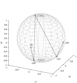
Figure 2: States obtained via general piecewise constant controls

In Figure 2 the lines indicate that the network system is taken from a point in $\mathbb{R}^{3}$ to another along some undetermined path on the unit sphere. Because $b_{2}$ is a negative number, $u_{2}$ is negative and, thus, $u_{2}$ is not a control pulse that represents the position of the switch.

4.2.2 Bang-bang controls I

Now algorithm 2 is applied to the preparation of $T_{1},$ $T_{2}$ and $T_{3}.$ As stated previously, the target $T_{1}$ can be prepared by free evolution and the target $T_{3}$ can be obtained with a control pulse of $1.$ Therefore, it remains to get bang-bang controls for $T_{2}$ so that the controls represent the position of the switch. It follows from equation (18) that

$$T_{2}=\exp\left(i\frac{\pi}{4}\sigma_{z}\right)=e^{-i\frac{7\pi}{4}\sigma_{y}}e^{i\frac{\pi}{4}\sigma_{x}}e^{-i\frac{\pi}{4}\sigma_{y}}.$$ (31)

Each of the three factors of equation (31) are of the form of (28), so that we have the following coefficients for $T_{2}$:

1π​52002π​1020π​102037​π​5200.fragments 1𝜋52002𝜋1020𝜋102037𝜋5200\begin{tabular}[]{c|c|c}$k$&$a_{k}$&$b_{k}$\\ \hline\cr$1$&$\frac{\pi\sqrt{5}}{20}$&$0$\\ $2$&$\frac{\pi\sqrt{10}}{20}$&$\frac{\pi\sqrt{10}}{20}$\\ $3$&$\frac{7\pi\sqrt{5}}{20}$&$0$\end{tabular}.

kakbkkakbk (32)

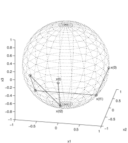
Figure 3: States obtained with bang-bang controls from algorithm 2

These coefficients represent bang-bang controls that drive the system as shown in Figure 3.

As in Figure 2, each line in Figure 3 represents the system being taken from one point in $\mathbb{R}^{3}$ to another along an undetermined path on the unit sphere. Controls having values of $0$ and $1$ to prepare $T_{2}$ can also be obtained by utilizing algorithm 3.

4.2.3 Bang-bang controls II

The preparation of $T_{1},$ $T_{2}$ and $T_{3}$ is now achieved by use of algorithm 3 to obtain controls of $0$ and $1$. Again, the target $T_{1}$ can be prepared by free evolution and the target $T_{3}$ can be obtained with a control pulse of $1.$ It remains to prepare $T_{2}=\exp\left(i\frac{\pi}{4}\sigma_{z}\right)$ by solving for $D$, $E$ and $F$ in the decomposition of $T$ given by equation(19). Equation (1) is used to find values for $\alpha$, $\zeta$ and $\mu.$ Since

$$T_{2}=\left(\begin{array}[]{cc}\exp\left(i\frac{\pi}{4}\right)&0\\ 0&\exp\left(-i\frac{\pi}{4}\right)\end{array}\right),$$ (33)

$\alpha=0,$ $\zeta=\frac{\pi}{4}$ and $\mu\in\left[0,2\pi\right).$ From equations (20), (21) and (22) we can choose $D=\frac{3\pi}{4}$, $E=-\frac{7\pi}{4}$ and $F=\frac{\pi}{4}.$ These values of $D$, $E$ and $F$ correspond to the following coefficients of $T_{2}$:

13​10​π203​10​π2027​5​π200310​π2010​π20.fragments 1310𝜋20310𝜋20275𝜋200310𝜋2010𝜋20\begin{tabular}[]{c|c|c}$k$&$a_{k}$&$b_{k}$\\ \hline\cr$1$&$\frac{3\sqrt{10}\pi}{20}$&$\frac{3\sqrt{10}\pi}{20}$\\ $2$&$\frac{7\sqrt{5}\pi}{20}$&$0$\\ $3$&$\frac{\sqrt{10}\pi}{20}$&$\frac{\sqrt{10}\pi}{20}$\end{tabular}.

kakbkkakbk (34)

Figure 4: States obtained with bang-bang controls from algorithm 3

The switched network system in $SO(3)$ is driven from $\mathbf{x}\left(t1\right)$ to $\mathbf{x}\left(t2\right)$ with these coefficients as shown in Figure 4. Each line in Figure 4 represents the system being taken from one point in $\mathbb{R}^{3}$ to another along an undetermined path on the unit sphere.

5 A Fourth Order Network

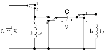
Figure 5: Fourth Order Switched Network

In this section a fourth order network (see Figure 5) taken from [11] is considered and it is shown how to effect certain state transfers via bang-bang controls. To the best of our knowledge these state transfers are the first instances of explicit exact control of systems with drift on $S^{3},$ the sphere in $\mathbb{R}^{4}.$ The system’s equations are:

$$\dot{x}=\left(\begin{array}[]{cccc}0&-\nu&0&0\\ \nu&0&0&0\\ 0&0&0&-\beta\\ 0&0&\beta&0\end{array}\right)x+\left(\begin{array}[]{cccc}0&0&0&\gamma\\ 0&0&\delta&0\\ 0&-\delta&0&0\\ -\gamma&0&0&0\end{array}\right)xu(t)=Ax+Bxu\left(t\right).$$ (35)

The coefficient matrices of the system belong to $so(4)$ and thus the system evolves on the sphere, $S^{3},$ in $\mathbb{R}^{4}$. The constants, $\nu,\beta,\gamma$ and $\delta$ are positive and are related to the inductances and capacitances of the elements of the circuits. Specifically, we have,

$$\nu=\frac{1}{\sqrt{L_{1}C_{2}}},\ \beta=\frac{1}{\sqrt{L_{3}C_{4}}},\ \gamma=\frac{1}{\sqrt{L_{1}C_{4}}},\ \delta=\frac{1}{\sqrt{L_{3}C_{2}}}.$$

Here $C_{1},C_{2}$ are the two capacitances and $L_{1},L_{3}$ are the two inductances in the circuit (See [11] for specific details). The state vector $\mathbf{x}=\left(x_{1},x_{2},x_{3},x_{4}\right)^{T}$ is defined as $x_{1}=\sqrt{L_{1}}I_{1}$, $x_{2}=\sqrt{C_{2}}V_{2}$, $x_{3}=\sqrt{L_{3}}I_{3}$ and $x_{4}=\sqrt{C_{4}}V_{4}$. To this system we can associate two systems whose unitary generators evolve on $SU(2)$ by using equations (3) - (5) of section 2:

$$\dot{U}_{1} = i\left(\frac{\nu+\beta}{2}\right)\sigma_{z}U_{1}-i\left(\frac{\gamma+\delta}{2}\right)\sigma_{x}U_{1}u(t),\quad U_{1}\text{ in }SU(2)$$

$$= A_{1}U_{1}+B_{1}U_{1}u(t)$$

and

$$\dot{U}_{2} = i\left(\frac{\beta-\nu}{2}\right)\sigma_{z}U_{2}+i\left(\frac{\gamma-\delta}{2}\right)\sigma_{x}U_{2}u(t),\quad U_{2}\text{\ in }SU(2)$$

$$= A_{2}U_{2}+B_{2}U_{2}u(t).$$

Note that both systems are controlled by the same control, $u(t)$.

The strategy to control the network is as follows. Supposed it is desired to transfer the state from $(1,0,0,0)^{T}$ to a vector $y$ in $S^{3}$, then one first represents $(1,0,0,0)^{T}$ and $y$ by the unit quaternions $1$ and $y$. The next step is to find a pair of unit quaternions $p$, $q$ such that $pq^{-1}=y$. To $p$ and $q$ there correspond matrices (denoted by $p$ and $q$ again) in $SU(2)$ (see section 2). We then try to find a $u(t)$ which will prepare, simultaneously, $p$ for system (5) and $q$ for system (5). In general there will be an infinite family $p$, $q$ such that $pq^{-1}=y$. To avail of this, we represent $p$ via equation (1) with $\alpha,\zeta,\mu$ floating. This will then determine $q$. The parameters $(\alpha,\zeta,\mu)$ are then found by the requirement that the same $u(t)$ prepare both $p$ and $q$. The details of this strategy, of course, depend on the specific sequence of piecewise constant controls which are used to prepare a state for a given system on $SU(2)$. Equivalently, they depend on the specific factorization of $SU(2)$ being employed.

We will now illustrate one such technique with $y=(0,0,1,0)^{T}$. The $SU(2)$ matrix corresponding to $y$ is $e^{i\frac{\pi}{2}\sigma_{y}}$. Thus, $pq^{-1}=e^{i\frac{\pi}{2}\sigma_{y}}$. It turns out that this strategy can be implemented if any one of the following conditions on the constants of the circuit holds:

$$\frac{\nu+\beta}{\beta-\nu}=2k+1=\frac{\gamma+\delta}{\delta-\gamma},\quad k=1,2,\ldots$$ (38)

The above conditions are, of course, artifices of the specific factorization of $SU(2)$ that will be presently employed. Note that these conditions imply that $C_{2}=C_{4}$ and that $\sqrt{\frac{L_{1}}{L_{3}}}=\frac{2k+2}{2k}$.

Representing $p$ as $S\left(\frac{\pi}{4},\frac{(2k+1)^{2}\pi}{4k(k+1)},-\frac{(2k+1)\pi}{4k(k+1)}\right)$ suffices. Indeed, one can now factorize $p$ as:

$$p = \exp\left(\frac{(2k+1)\pi}{2(k+1)(\nu+\beta)}A_{1}\right)\exp\left(\frac{(2k+1)\pi}{\sqrt{2}(\nu+\beta)}A_{1}+\frac{(2k+1)\pi}{\sqrt{2}(\delta+\gamma)}B_{1}\right)$$ (39)

$$\cdot\exp\left(\frac{(2k+1)\left(6k+1\right)\pi}{2k\left(\nu+\beta\right)}A_{1}\right).$$

Since $q$ is determined by $p$ it follows that it can be factorized as:

$$q = \exp\left(\frac{\pi}{2(k+1)(\beta-\nu)}A_{2}\right)\exp\left(\frac{\pi}{\sqrt{2}(\beta-\nu)}A_{2}+\frac{\pi}{\sqrt{2}(\delta-\gamma)}B_{2}\right)$$ (40)

$$\cdot\exp\left(\frac{(6k+1)\pi}{2k\left(\beta-\nu\right)}A_{2}\right).$$

Using equation (38) it follows that the coefficients of $A_{1}$ match those of $A_{2}$ and similarly the coefficients of $B_{1}$ match those of $B_{2}$. Since these coefficients represent the duration and power of the pieces of the control $u(t)$, it follows that the same control, $u(t)$ prepares both $p$ and $q$ and thus achieves the desired state for the circuit. Furthermore, the controls are indeed bang-bang with values $1$ or $0$. This follows from equation (38) which forces, $\frac{\delta+\gamma}{\nu+\beta}=1$ (keeping in mind the relation of these constants to the inductances and capacitances).

Several remarks are in order at this stage:

1. $k=0$ was omitted from (38) since it would be physically unreasonable;

2. Using similar ideas, it can be shown that under equation (38), an explicit pulse sequence can be found for state transfer from $(1,0,0,0)^{T}$ to any of the following states: $\pm(0,1,0,0)^{T},\pm(0,0,1,0)^{T},\pm(0,0,0,1)^{T}$. Furthermore, this holds also when equation (38) is modified to $\left|\frac{\nu+\beta}{\beta-\nu}\right|=2k+1=\left|\frac{\gamma+\delta}{\gamma-\delta}\right|,\ k=1,2,\ldots$ For this it is useful to note that the Cayley-Klein representation (1), need not necessarily be the polar coordinates of the entries. Indeed, since $e^{i\pi}=e^{-i\pi}=-1$, one can begin with polar coordinates and yet dispense with the restriction that $\alpha$ be in $[0,\frac{\pi}{2}]$. To illustrate this, consider transferring the state from $(1,0,0,0)^{T}$ to $(0,0,0,1)^{T}.$ Suppose equation (38) is replaced with

   $$\frac{\nu+\beta}{\beta-\nu}=2k+1;\quad\frac{\gamma+\delta}{\delta-\gamma}=-\left(2k+1\right),\quad k=1,2,\ldots$$ (41)

   Now $pq^{-1}=e^{i\frac{\pi}{2}\sigma_{x}}.$ So if $p=S\left(\alpha,\zeta,\mu\right),$ then

   $$q=S\left(\alpha-\frac{\pi}{2},\frac{\pi}{2}-\mu,\frac{5\pi}{2}-\zeta\right).$$ (42)

   It suffices to choose $p=S\left(\frac{\pi}{4},\frac{(2k+1)\left(5k+2\right)\pi}{4k\left(k+1\right)},\frac{(2k+1)\left(k-2\right)\pi}{4k\left(k+1\right)}\right).$ Indeed, this $p$ can be factorized as

   $$p = \exp\left(\frac{(2k+1)3\pi}{2(k+1)(\nu+\beta)}A_{1}\right)\exp\left(\frac{(2k+1)\pi}{\sqrt{2}(\nu+\beta)}A_{1}+\frac{(2k+1)\pi}{\sqrt{2}(\delta+\gamma)}B_{1}\right)$$ (43)

   $$\cdot\exp\left(\frac{(2k+1)\left(10k+2\right)\pi}{2k\left(\nu+\beta\right)}A_{1}\right).$$

   Similarly, $q$ can be factorized as

   $$q = \exp\left(\frac{3\pi}{2(k+1)(\beta-\nu)}A_{2}\right)\exp\left(\frac{\pi}{\sqrt{2}(\beta-\nu)}A_{2}+\frac{\pi}{\sqrt{2}(\gamma-\delta)}B_{2}\right)$$ (44)

   $$\cdot\exp\left(\frac{(10k+2)\pi}{2k\left(\beta-\nu\right)}A_{2}\right).$$

   Thus the same control which prepares $p$ does likewise for $q.$ Once again, this control is a bang-bang control with values 0 and 1;

3. The state $(0,1,0,0)^{T}$ can be prepared by free evolution without any conditions on the circuit. This is not evident from equation (35), without the calculation of an exponential. On the other hand, since $(0,1,0,0)^{T}$ is equivalent to $e^{i\frac{\pi}{2}\sigma_{z}},$ it follows with minimal fuss upon passage to $SU(2),$ i.e., with no calculation whatsoever. Indeed, the matrices $A_{1}$ and $A_{2}$ from equations (5) and (5) are (different) multiples of $i\sigma_{z}.$ Hence it suffices to choose the targets $p$ and $q$ of systems (5) and (5) as $p=e^{iL\sigma_{z}}$ and $q=e^{i\left(L-\frac{\pi}{2}\right)\sigma_{z}},$ for some $L$ determined by

   $$\frac{L}{\nu+\beta}=\frac{L-\frac{\pi}{2}}{\beta-\nu}.$$

   This $p$ and $q,$ and hence $(0,1,0,0)^{T},$ can obviously be prepared by free evolution. Note, this conclusion did not even require an $su\left(2\right)$ exponential.

4. For final states other than those in ii), we believe the same idea is viable. The resultant equations for the Cayley-Klein parameters of $p$ now are transcendental [4]. Intuitively, it seems plausible that these equations can be solved since $SO\left(4\right)$ acts transitively on the 3-sphere, $S^{3},$ with isotropy given by $SO\left(3\right).$ As $SO\left(3\right)$ is nearly $SU(2),$ it seems reasonable to expect success of the strategy of finding, parametrically, a suitable $p$ in $SU(2)$ to ensure that the same $u(t)$ will prepare both $p$ and $q$;

5. The conditions imposed by equation (38) or (41) can be met in practice. Nevertheless, it would be useful to achieve state transfers without this restriction. For this, different factorizations of $SU(2)$ need to be developed;

6. The factorizations in equations (39), (40), (43) and (44) are not Euler factorizations. Even though three factors appear in each of these expressions, it is clear that $A_{i}$ is not orthogonal to a linear combination of $A_{i}$ and $B_{i},$ $i=1,2.$ Thus, these factorizations are not Euler factorizations. Without passage to $SU(2),$ it seems formidable to find similar factorizations directly for $SO\left(4\right).$

6 Conclusions

Lossless networks of the type studied in this paper are important in many applications. Therefore, a constructive strategy for preparing desired states in such circuits is interesting. In this paper the novel technique of using factorizations of the special unitary group $SU(2)$ was shown to be a viable mechanism for this issue. The key enabling factor is the rich algebraic structure of $su(2).$ Finding similar formulae for $so(3)$ and $so(4)$ directly is harder. However, once a formula on $SU(2)$ has been found - whether it be for exponentials, bang-bang controls etc., - it can be transferred with ease to the orthogonal group. This is the rationale behind our method. While the individual properties of the networks played an important role in the success of the methodology, the basic idea of using factorizations of $SU(2)$ is a useful complement to other methods for dealing with systems evolving on the unitary and orthogonal matrices. Indeed, for the treatment of systems with drift, techniques based on decompositions of unitary groups appear to be more viable. It seems reasonable to expect that similar methods should work for other systems evolving on the orthogonal groups. For instance, $so(6)$ is isomorphic to $su(4)$. The latter Lie algebra plays an important role in quantum control.

References

• [1] B. Adams, Algebraic Approach to Simple Quantum Systems, Springer-Verlag, New York, 1999.
• [2] R. Brockett and J. Wood, Electrical Networks Containing Controlled Switches, Applications of Lie Group Theory to Nonlinear Network Problems, pp. 1-11, Western Periodicals Co., 1974.
• [3] K. Flores, Thesis. In preparation.
• [4] K. Flores and V. Ramakrishna, Quantum Control Techniques for Switched Electrical Networks Having Four Circuit Elements, University of Texas at Dallas, Center for Systems, Signals and Telecommunications, Technical Report.
• [5] R. Horn and C. Johnson, Topics in Matrix Analysis, Academic Press, 1980.
• [6] V. Jurdjevic and H. Sussmann, Control Systems on Lie Groups. Journal of Differential Equations, 12, 313, 1972.
• [7] N. Leonard and P. Krishnaprasad, Control of Switched Electrical Networks on Lie Groups, Proceedings of the 31st IEEE Control and Decision Conference, 1230, IEEE Press, Piscataway, NJ.
• [8] V. Ramakrishna, K. Flores, H. Rabitz, R. Ober, Quantum Control by Decompositions of $SU(2),$ Phys. Rev. A., 62, 053409-1-5, Oct. 13, 2000.
• [9] V. Ramakrishna, et. al, Explicit Generation of Unitary Transformations in a Single Atom/Molecule, Phys. Rev. A., 61, 032106-1-6, Feb. 28, 2000.
• [10] H. Sira-Ramirez, Sliding Motions in Bilinear Switched Networks, IEEE Transactions on Circuits and Systems, 34(8), 919, 1987.
• [11] J. Wood, Power Conversion in Electrical Networks, Technical Report NASA Rep. No. CR-120830, 1973. Also PhD thesis, Harvard University, 1974.