NONLINEAR DYNAMICS OF HIGH-BRIGHTNESS BEAMS

Abstract

The consideration of transverse dynamics of relativistic space-charge dominated beams and halo growth due to bunch oscillations is based on variational approach to rational (in dynamical variables) approximation for rms envelope equations. It allows to control contribution from each scale of underlying multiscales and represent solutions via exact nonlinear eigenmodes expansions. Our approach is based on methods provided possibility to work with well-localized bases in phase space and good convergence properties of the corresponding expansions.

1 Introduction

In this paper we consider the applications of a new numerical-analytical technique based on the methods of local nonlinear harmonic analysis or wavelet analysis to nonlinear rms envelope dynamics problems which can be characterized by collective type behaviour [1], [2]. Such approach may be useful in all models in which it is possible and reasonable to reduce all complicated problems related with statistical distributions to the problems described by systems of nonlinear ordinary/partial differential equations with or without some (functional) constraints. Wavelet analysis is a set of mathematical methods, which gives the possibility to work with well-localized bases in functional spaces and gives the maximum sparse forms for the general type of operators (differential, integral, pseudodifferential) in such bases. Our approach is based on the variational-wavelet approach from [3]-[14], that allows to consider rational type of nonlinearities in rms dynamical equations. The solution has the multiscale/multiresolution decomposition via nonlinear high-localized eigenmodes, which corresponds to the full multiresolution expansion in all underlying time/space scales. We may move from coarse scales of resolution to the finest one for obtaining more detailed information about our dynamical process. In this way we give contribution to our full solution from each scale of resolution or each time/space scale or from each nonlinear eigenmode. The same is correct for the contribution to power spectral density (energy spectrum): we can take into account contributions from each level/scale of resolution. Starting in part 2 from general rms envelope dynamics model we consider in part 3 the approach based on variational-wavelet formulation. We give explicit representation for all dynamical variables in the base of compactly supported wavelets or nonlinear eigenmodes. Our solutions are parametrized by the solutions of a number of reduced algebraical problems one from which is nonlinear with the same degree of nonlinearity and the others are the linear problems depend on particular wavelet type approach. In part 4 we consider numerical modelling based on our analytical approach.

2 RMS EQUATIONS

We consider an approach based on the second moments of the distribution functions for the calculation of evolution of rms envelope of a beam. The rms envelope equations are the most useful for analysis of the beam self–forces (space–charge) effects and also allow to consider both transverse and longitudinal dynamics of space-charge-dominated relativistic high–brightness axisymmetric/asymmetric beams, which under short laser pulse–driven radio-frequency photoinjectors have fast transition from nonrelativistic to relativistic regime [1]. The analysis of halo growth in beams, appeared as result of bunch oscillations in the particle-core model, is also based on three-dimensional envelope equations [1], [2]. Let $f(x_{i})$ be the distribution function, which gives full information about noninteracting ensemble of beam particles regarding to trace space or transverse phase coordinates $(x_{i},x_{j})$. Then we may extract the first nontrivial effects of collective dynamics from the second moments

$$\sigma_{x_{i}x_{j}}^{2}=<x_{i}x_{j}>=\int\int x_{i}x_{j}f(x)\mathrm{d}x_{i}\mathrm{d}x_{j}$$ (1)

RMS emittances are given by

$$\varepsilon^{2}_{x_{i},rms}=<x_{i}^{2}><\dot{x}_{i}^{2}>-<x_{i}\dot{x}_{i}>^{2}$$ (2)

We consider the following most general case of rms envelope equations, which describe evolution of the moments in the model of halo formation by bunch oscillations (ref. [2] for full designation):

$$\ddot{\sigma}_{x}+k_{x}^{2}(s)\sigma_{x}-\frac{\xi_{x}}{\sigma_{y}\sigma_{z}}-\frac{\varepsilon^{2}_{x}}{\sigma_{x}^{3}} = 0,$$

$$\ddot{\sigma}_{y}+k_{y}^{2}(s)\sigma_{y}-\frac{\xi_{y}}{\sigma_{x}\sigma_{z}}-\frac{\varepsilon^{2}_{y}}{\sigma_{y}^{3}} = 0,$$ (3)

$$\ddot{\sigma}_{z}+k_{z}^{2}(s)\sigma_{z}-\gamma^{2}\frac{\xi_{z}}{\sigma_{x}\sigma_{y}}-\frac{\varepsilon^{2}_{z}}{\sigma_{z}^{3}} = 0,$$

where $\sigma_{x}(s),\sigma_{y}(s),\sigma_{z}(s)$ are bunch envelopes, $\xi_{x},\xi_{y}$, $\xi_{z}=F(\sigma_{x},\sigma_{y},\sigma_{z})$. After transformations to Cauchy form we can see that all these equations from the formal point of view are not more than ordinary differential equations with rational nonlinearities and variable coefficients. Also, we consider regimes in which we are interested in constraints on emittances:

$$\varepsilon^{2}_{x_{i},rms}=c_{i},$$ (4)

where $c_{i}$ are constants. In the same way according to [2] we may consider the case of energy-type functional-differential constraints on emittances. A different approach is considered in our related paper in this Proceedings [15].

3 RATIONAL DYNAMICS WITH CONSTRAINTS

Our problems above may be formulated as the systems of ordinary differential equations

$$Q_{i}(x)\frac{\mathrm{d}x_{i}}{\mathrm{d}t}=P_{i}(x,t),\quad x=(x_{1},...,x_{n}),$$ (5)

$$i=1,...,n,\quad\max_{i}deg\ P_{i}=p,\quad\max_{i}deg\ Q_{i}=q$$

with initial (or boundary) conditions $x_{i}(0)$, $x_{i}(T)$ and $P_{i},Q_{i}$ are not more than polynomial functions of dynamical variables $x_{j}$ and have arbitrary dependence on time/length parameter. Of course, we consider such $Q_{i}(x)$ which do not lead to the singular problem with $Q_{i}(x)$, when $t=0$ or $t=T$, i.e. $Q_{i}(x(0)),Q_{i}(x(T))\neq\infty$, 0. We’ll consider these equations as the following operator equation. Let $L$ be an arbitrary nonlinear (rational) matrix differential operator of the first order with matrix dimension d (d=6 in our case) corresponding to the system of equations (5), which acts on some set of functions $\Psi\equiv\Psi(t)=\Big{(}\Psi^{1}(t),\dots,\Psi^{d}(t)\Big{)},\quad t\in\Omega\subset R$ from $L^{2}(\Omega)$:

$$L\Psi\equiv L(R,t)\Psi(t)=0,$$ (6)

where $R\equiv R(t,\partial/\partial t,\Psi)$.

Let us consider now the N mode approximation for solution as the following ansatz (in the same way we may consider different ansatzes):

$$\Psi^{N}(t)=\sum^{N}_{r=1}a^{N}_{r}\psi_{r}(t)$$ (7)

We shall determine the coefficients of expansion from the following variational conditions (different related variational approaches are considered in [3]-[14]):

$$L^{N}_{k}\equiv\int(L\Psi^{N})\psi_{k}(t)\mathrm{d}t=0$$ (8)

We have exactly $dN$ algebraical equations for $dN$ unknowns $a_{r}$. So, variational approach reduced the initial problem (5) or (6) to the problem of solution of functional equations at the first stage and some algebraical problems at the second stage. Here $\psi_{k}(t)$ are useful basis functions of some functional space ($L^{2},L^{p}$, Sobolev, etc) corresponding to concrete problem. As result we have the following reduced algebraical system of equations (RSAE) on the set of unknown coefficients $a_{i}^{N}$ of expansions (7):

$$L(Q_{ij},a_{i}^{N},\alpha_{I})=M(P_{ij},a_{i}^{N},\beta_{J}),$$ (9)

where operators L and M are algebraization of RHS and LHS of initial problem (5). $Q_{ij}$ are the coefficients (with possible time dependence) of LHS of initial system of differential equations (5) and as consequence are coefficients of RSAE. $P_{ij}$ are the coefficients (with possible time dependence) of RHS of initial system of differential equations (5) and as consequence are the coefficients of RSAE. $I=(i_{1},...,i_{q+2})$, $J=(j_{1},...,j_{p+1})$ are multiindexes, by which are labelled $\alpha_{I}$ and $\beta_{I}$, the other coefficients of RSAE (9):

$$\beta_{J}=\{\beta_{j_{1}...j_{p+1}}\}=\int\prod_{1\leq j_{k}\leq p+1}\psi_{j_{k}},$$ (10)

where p is the degree of polynomial operator P (5)

$$\alpha_{I}=\{\alpha_{i_{1}}...\alpha_{i_{q+2}}\}=\sum_{i_{1},...,i_{q+2}}\int\psi_{i_{1}}...\dot{\psi_{i_{s}}}...\psi_{i_{q+2}},$$ (11)

where q is the degree of polynomial operator Q (5), $i_{\ell}=(1,...,q+2)$, $\dot{\psi_{i_{s}}}=\mathrm{d}\psi_{i_{s}}/\mathrm{d}t$.

According to [3]-[14] we may extend our approach to the case when we have additional constraints (4) on the set of our dynamical variables $\Psi$ or $x$. In this case by using the method of Lagrangian multipliers we again may apply the same approach but for the extended set of variables. As result we receive the expanded system of algebraical equations analogous to the system (9). Then, after reduction we again can extract from its solution the coefficients of expansion (7). Now, when we solve RSAE (9) and determine unknown coefficients from formal expansion (7) we therefore obtain the solution of our initial problem. It should be noted if we consider only truncated expansion (7) with N terms then we have from (9) the system of $N\times d$ algebraical equations with degree $\ell=max\{p,q\}$ and the degree of this algebraical system coincides with degree of initial differential system. So, we have the solution of the initial nonlinear (rational) problem in the form

$$x(t)=x(0)+\sum_{k=1}^{N}a_{k}^{N}\psi_{k}(t),$$ (12)

where coefficients $a_{k}^{N}$ are roots of the corresponding reduced algebraical (polynomial) problem RSAE (9). Consequently, we have a parametrization of solution of initial problem by solution of reduced algebraical problem (9).

The problem of computations of coefficients $\alpha_{I}$ (11), $\beta_{J}$ (10) of reduced algebraical system may be explicitly solved in wavelet approach. The obtained solutions are given in the form (12), where $\psi_{k}(t)$ are wavelet basis functions. In our case $\psi_{k}(t)$ are obtained via multiresolution expansions and represented by compactly supported wavelets. Because affine group of translation and dilations is inside the approach, this method resembles the action of a microscope. We have contribution to final result from each scale of resolution from the whole infinite scale of spaces:

$$...V_{-2}\subset V_{-1}\subset V_{0}\subset V_{1}\subset V_{2}\subset...,$$

where the closed subspace $V_{j}(j\in{\bf Z})$ corresponds to level j of resolution, or to scale j. This multiresolution functional space decomposition corresponds to exact nonlinear eigenmode decompositions (12).

It should be noted that such representations give the best possible localization properties in the corresponding (phase)space/time coordinates. In contrast with different approaches formulae (7), (12) do not use perturbation technique or linearization procedures and represent dynamics via generalized nonlinear localized eigenmodes expansion. So, by using wavelet bases with their good (phase)space/time localization properties we can construct high-localized (coherent) structures in spatially-extended stochastic systems with collective behaviour.

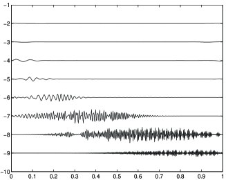
Figure 1: Multiscale decomposition.

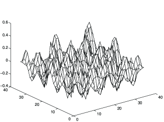
Figure 2: $\sigma_{x}$–$\sigma_{y}$ section.

4 Modelling

So, our N mode construction (7), (12) gives the following representation for solution of rms equations (3):

$$x(t) = x_{N}^{slow}(t)+\sum_{i\geq N}x^{i}(\omega_{i}t),\quad\omega_{i}\sim 2^{i}$$ (13)

where $x^{r}(s)$ may be represented by some family of (nonlinear) eigenmodes and gives as a result the multiresolution/multiscale representation in the high-localized wavelet bases. The corresponding decomposition is presented on Fig. 1 and two-dimensional transverse section $\sigma_{x}$–$\sigma_{y}$ on Fig. 2.

5 Acknowledgments

We would like to thank The U.S. Civilian Research & Development Foundation (CRDF) for support (Grants TGP-454, 455), which gave us the possibility to present our nine papers during PAC2001 Conference in Chicago and Ms.Camille de Walder from CRDF for her help and encouragement.

References

- [1] The Physics of High Brightness Beams, Ed.J. Rosenzweig & L. Serafini, World Scientific, 2000.
- [2] C. Allen, paper in [1], p. 173, I. Hofmann, CERN Proc. 95-06, vol.2, 941, 1995.
- [3] A.N. Fedorova and M.G. Zeitlin, Math. and Comp. in Simulation, 46, 527, 1998.
- [4] A.N. Fedorova and M.G. Zeitlin, New Applications of Nonlinear and Chaotic Dynamics in Mechanics, 31, 101 Kluwer, 1998.
-
[5]
A.N. Fedorova and M.G. Zeitlin,
CP405, 87, American Institute of Physics, 1997.
Los Alamos preprint,
physics/9710035. - [6] A.N. Fedorova, M.G. Zeitlin and Z. Parsa, Proc. PAC97 2, 1502, 1505, 1508, APS/IEEE, 1998.
- [7] A.N. Fedorova, M.G. Zeitlin and Z. Parsa, Proc. EPAC98, 930, 933, Institute of Physics, 1998.
- [8] A.N. Fedorova, M.G. Zeitlin and Z. Parsa, CP468, 48, American Institute of Physics, 1999. Los Alamos preprint, physics/990262.
- [9] A.N. Fedorova, M.G. Zeitlin and Z. Parsa, CP468, 69, American Institute of Physics, 1999. Los Alamos preprint, physics/990263.
-
[10]
A.N. Fedorova and M.G. Zeitlin,
Proc. PAC99,
1614, 1617, 1620, 2900, 2903,
2906, 2909, 2912, APS/IEEE, New York, 1999.
Los Alamos preprints: physics/9904039, 9904040,
9904041, 9904042, 9904043, 9904045, 9904046, 9904047. - [11] A.N. Fedorova and M.G. Zeitlin, The Physics of High Brightness Beams, 235, World Scientific, 2000. Los Alamos preprint: physics/0003095.
-
[12]
A.N. Fedorova and M.G. Zeitlin, Proc. EPAC00, 415, 872, 1101, 1190, 1339, 2325,Austrian Acad.Sci.,2000.
Los Alamos preprints: physics/0008045, physics/0008046,
physics/0008047, physics/0008048, physics/0008049,
physics/0008050. - [13] A.N. Fedorova, M.G. Zeitlin, Proc. 20 International Linac Conf., 300, 303, SLAC, Stanford, 2000. Los Alamos preprints: physics/0008043, physics/0008200.
-
[14]
A.N. Fedorova, M.G. Zeitlin, Los Alamos preprints:
physics/0101006, physics/0101007 and World Scientific, in press. - [15] A.N. Fedorova, M.G. Zeitlin, Space-charge Dominated Beam Transport via Multiresolution, this Proc..