SPACE-CHARGE DOMINATED BEAM TRANSPORT VIA MULTIRESOLUTION

Abstract

We consider space-charge dominated beam transport systems, where space-charge forces are the same order as external focusing forces and dynamics of the corresponding emittance growth. We consider the coherent modes of oscillations and coherent instabilities both in the different nonlinear envelope models and in initial collective dynamics picture described by Vlasov system. Our calculations are based on variation approach and multiresolution in the base of high-localized generalized coherent states/wavelets. We control contributions to dynamical processes from underlying multiscales via nonlinear high-localized eigenmodes expansions in the base of compactly supported wavelet and wavelet packets bases.

1 INTRODUCTION

In this paper we consider the applications of a new numerical-analytical technique based on wavelet analysis approach for calculations related to description of different space-charge effects. We consider models for space-charge dominated beam transport systems in case when space-charge forces are the same order as external focusing forces and dynamics of the corresponding emittance growth related with oscillations of underlying coherent modes [1],[2]. Such approach may be useful in all models in which it is possible and reasonable to reduce all complicated problems related with collective behaviour and corresponding statistical distributions to the problems described by systems of nonlinear ordinary/partial differential equations. Also we consider an approach based on the second moments of the distribution functions for the calculation of evolution of rms envelope of a beam. The rational type of nonlinearities allows us to use our results from [3]-[14], which are based on the application of wavelet analysis technique to variational formulation of initial nonlinear problems. Wavelet analysis is a set of mathematical methods, which gives us a possibility to work with well-localized bases in functional spaces and give for the general type of operators (differential, integral, pseudodifferential) in such bases the maximum sparse forms. In part 2 we describe the approach based on Vlasov-type model and corresponding rms equations. In part 3 we present explicit analytical construction for solutions of Vlasov (besides gaussians) and rms equations from part 2, which are based on variational formulation of initial dynamical problems, multiresolution representation and fast wavelet transform technique [15]. We give explicit representation for all dynamical variables in the base of high-localized generalized coherent states/wavelets. Our solutions are parametrized by solutions of a number of reduced algebraical problems one from which is nonlinear with the same degree of nonlinearity and the others are the linear problems which come from the corresponding wavelet constructions. In part 4 we present results of numerical calculations.

2 VLASOV/RMS EQUATIONS

Let ${\bf x}(s)=\big{(}x_{1}(s),x_{2}(s)\big{)}$ be the transverse coordinates, then single-particle equation of motion is (ref.[1] for designations):

$${\bf x}^{\prime\prime}+\mathbf{k}_{\bf x}(s){\bf x}-D\mathbf{E}_{\mathbf{x}}({\bf x},s)=0,$$ (1)

where $D=q/{m\gamma^{3}v_{0}^{2}}$, $\ \mathbf{k}_{\mathbf{x}}(s)$ describes periodic focusing force and $\mathbf{E}$ satisfies the Poisson equation:

$$\nabla\cdot{\bf E}=\frac{q}{\varepsilon_{0}}n({\bf x},s)$$ (2)

with the following density projection:

$$n=\int\int f({\bf x},{\bf x}^{\prime},s)\mathrm{d}{\bf x}^{\prime}$$ (3)

Distribution function $f(\mathbf{x},\mathbf{x}^{\prime})$ satisfies Vlasov equation

$$\frac{\partial f}{\partial s}+({\bf x}^{\prime}\cdot\nabla)f-\Big{(}{\bf k}-D{\bf E}\Big{)}\cdot\nabla_{\bf x^{\prime}}f=0$$ (4)

Using standard procedure, which takes into account that rms emittance is described by the seconds moments only

$$\varepsilon^{2}_{x,rms}=<x_{i}^{2}><x_{j}^{2}>-<x_{i}x_{j}>^{2}(i\neq j),$$

we arrive to the beam envelope equations for $\sigma_{x_{i}}$:

$$\sigma_{x_{1}}^{\prime\prime}+k_{x_{1}}(s)\sigma_{x_{1}}-\varepsilon^{2}_{x_{1}}/\sigma_{x_{1}}^{3}-C/(\sigma_{x_{1}}+\sigma_{x_{2}}) = 0$$ (5)

$$\sigma_{x_{2}}^{\prime\prime}+k_{x_{2}}(s)\sigma_{x_{2}}-\varepsilon^{2}_{x_{2}}/\sigma_{x_{2}}^{3}-C/(\sigma_{x_{1}}+\sigma_{x_{2}}) = 0,$$

where $C=qI/\pi\varepsilon_{0}m\gamma^{3}v_{0}^{2}$ but only in case when we can calculate explicitly $<x_{i}E_{j}>$. An additional equation describes evolution of $\varepsilon^{2}_{x_{i}}(s)$:

$$\frac{\mathrm{d}\varepsilon_{x}^{2}}{\mathrm{d}s}=32D\big{(}<x_{i}^{2}><x_{j}E_{i}>-<x_{i}x_{j}><x_{i}E_{i}>\big{)}$$

For nonlinear $E_{i}$ we need higher order moments, which lead to infinite system of equations. These rms-type envelope equations, from the formal point of view, are not more than nonlinear differential equations with rational nonlinearities and variable coefficients.

3 WAVELET REPRESENTATIONS

One of the key points of wavelet approach demonstrates that for a large class of operators wavelets are good approximation for true eigenvectors and the corresponding matrices are almost diagonal. Fast wavelet transform gives the maximum sparse form of operators under consideration. It is true also in case of our Vlasov-type system of equations (1)-(4). We have both differential and integral operators inside. So, let us denote our (integral/differential) operator from equations (1)-(4) as $T$ and his kernel as $K$. We have the following representation:

$$<Tf,g>=\int\int K(x,y)f(y)g(x)\mathrm{d}x\mathrm{d}y$$ (6)

In case when $f$ and $g$ are wavelets $\varphi_{j,k}=2^{j/2}\varphi(2^{j}x-k)$ (7) provides the standard representation of operator $T$. Let us consider multiresolution representation

$$\dots\subset V_{2}\subset V_{1}\subset V_{0}\subset V_{-1}\subset V_{-2}\dots$$

The basis in each $V_{j}$ is $\varphi_{j,k}(x)$, where indices $\ k,j$ represent translations and scaling respectively or the action of underlying affine group which act as a “microscope” and allow us to construct corresponding solution with needed level of resolution. Let $T$ act : $L^{2}(R^{n})$ $\rightarrow L^{2}(R^{n})$, with the kernel $K(x,y)$ and $P_{j}:L^{2}(R^{n})\rightarrow V_{j}$ $(j\in Z)$ is projection operators on the subspace $V_{j}$ corresponding to j level of resolution:

$$(P_{j}f)(x)=\sum_{k}<f,\varphi_{j,k}>\varphi_{j,k}(x).$$

Let $Q_{j}=P_{j-1}-P_{j}$ be the projection operator on the subspace $W_{j}$ then we have the following ”microscopic or telescopic” representation of operator T which takes into account contributions from each level of resolution from different scales starting with coarsest and ending to finest scales [15]:

$$T=\sum_{j\in Z}(Q_{j}TQ_{j}+Q_{j}TP_{j}+P_{j}TQ_{j}).$$

We remember that this is a result of presence of affine group inside this construction. The non-standard form of operator representation [15] is a representation of operator T as a chain of triples $T=\{A_{j},B_{j},\Gamma_{j}\}_{j\in Z}$, acting on the subspaces $V_{j}$ and $W_{j}$:

$$A_{j}:W_{j}\rightarrow W_{j},B_{j}:V_{j}\rightarrow W_{j},\Gamma_{j}:W_{j}\rightarrow V_{j},$$

where operators $\{A_{j},B_{j},\Gamma_{j}\}_{j\in Z}$ are defined as $A_{j}=Q_{j}TQ_{j},\quad B_{j}=Q_{j}TP_{j},\quad\Gamma_{j}=P_{j}TQ_{j}.$ The operator $T$ admits a recursive definition via

$$T_{j}=\left(\begin{array}[]{cc}A_{j+1}&B_{j+1}\\ \Gamma_{j+1}&T_{j+1}\end{array}\right),$$

where $T_{j}=P_{j}TP_{j}$ and $T_{j}$ works on $V_{j}:V_{j}\rightarrow V_{j}$. It should be noted that operator $A_{j}$ describes interaction on the scale $j$ independently from other scales, operators $B_{j},\Gamma_{j}$ describe interaction between the scale j and all coarser scales, the operator $T_{j}$ is an ”averaged” version of $T_{j-1}$. We may compute such non-standard representations of operator for different operators (including pseudodifferential). As in case of differential operator $\mathrm{d}/\mathrm{d}x$ as in other cases in the wavelet bases we need only to solve the system of linear algebraical equations. Let

$$r_{\ell}=\int\varphi(x-\ell)\frac{\mathrm{d}}{\mathrm{d}x}\varphi(x)\mathrm{d}x,\ell\in Z.$$

Then, the representation of $d/dx$ is completely determined by the coefficients $r_{\ell}$ or by representation of $d/dx$ only on the subspace $V_{0}$. The coefficients $r_{\ell},\ell\in Z$ satisfy the usual system of linear algebraical equations. For the representation of operator $d^{n}/dx^{n}$ or integral operators we have the similar reduced linear system of equations. Then finally we have for action of operator $T_{j}(T_{j}:V_{j}\rightarrow V_{j})$ on sufficiently smooth function $f$:

$$(T_{j}f)(x)=\sum_{k\in Z}\left(2^{-j}\sum_{\ell}r_{\ell}f_{j,k-\ell}\right)\varphi_{j,k}(x),$$

where $\varphi_{j,k}(x)=2^{-j/2}\varphi(2^{-j}x-k)$ is wavelet basis and

$$f_{j,k-1}=2^{-j/2}\int f(x)\varphi(2^{-j}x-k+\ell)\mathrm{d}x$$

are wavelet coefficients. So, we have simple linear parametrization of matrix representation of our operators in wavelet bases and of the action of this operator on arbitrary vector in our functional space. Then we may apply our approach from [3]-[14]. For constructing the solutions of rms type equations (5),(6) obtained from Vlasov equations we also use our variational approach, which reduces initial problem to the problem of solution of functional equations at the first stage and some algebraical problems at the second stage. We have the solution in a compactly supported wavelet basis. Multiresolution representation is the second main part of our construction. The solution is parameterized by solutions of two reduced algebraical problems, one is nonlinear and the second are some linear problems, which are obtained from one of the wavelet constructions. The solution of equations (5),(6) has the following form

$$z(s)=z_{N}^{slow}(s)+\sum_{j\geq N}z_{j}(\omega_{j}s),\quad\omega_{j}\sim 2^{j}$$ (7)

which corresponds to the full multiresolution expansion in all underlying scales. Formula (7) gives us expansion into a slow part $z_{N}^{slow}$ and fast oscillating parts for arbitrary N. So, we may move from coarse scales of resolution to the finest one to obtain more detailed information about our dynamical process. The first term in the RHS of representation (8) corresponds on the global level of function space decomposition to resolution space and the second one to detail space. In this way we give contribution to our full solution from each scale of resolution or each time scale. It should be noted that such representations (8) give the best possible localization properties in phase space. This is especially important because our dynamical variables correspond to distribution functions/moments of ensemble of beam particles.

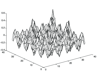
Figure 1: 6-eigenmodes representation.

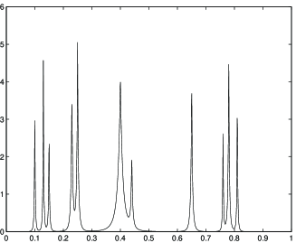
Figure 2: Region of nonlinear resonances.

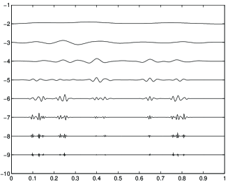
Figure 3: Eigenmodes decomposition.

4 Numerical Calculations

Now we present numerical illustrations of previous analytical approach. Numerical calculations are based on compactly supported wavelets and related wavelet families. Fig. 1 demonstrates 6-scale/eigenmodes construction for solution of equations (4). Figures 2,3 demonstrate resonances region and corresponding nonlinear coherent eigenmodes decomposition according to equation (8) [16].

5 ACKNOWLEDGMENTS

We would like to thank The U.S. Civilian Research & Development Foundation (CRDF) for support (Grants TGP-454, 455), which gave us the possibility to present our nine papers during PAC2001 Conference in Chicago and Ms.Camille de Walder from CRDF for her help and encouragement.

References

- [1] I. Hofmann, CERN Proc.95-06, vol.2, 941, 1995
- [2] The Physics of High Brightness Beams, Ed.J. Rosenzweig & L. Serafini, World Scientific, 2000
- [3] A.N. Fedorova and M.G. Zeitlin, Math. and Comp. in Simulation, 46, 527, 1998.
- [4] A.N. Fedorova and M.G. Zeitlin, New Applications of Nonlinear and Chaotic Dynamics in Mechanics, 31, 101 Kluwer, 1998.
-
[5]
A.N. Fedorova and M.G. Zeitlin,
CP405, 87, American Institute of Physics, 1997.
Los Alamos preprint,
physics/9710035. - [6] A.N. Fedorova, M.G. Zeitlin and Z. Parsa, Proc. PAC97 2, 1502, 1505, 1508, APS/IEEE, 1998.
- [7] A.N. Fedorova, M.G. Zeitlin and Z. Parsa, Proc. EPAC98, 930, 933, Institute of Physics, 1998.
- [8] A.N. Fedorova, M.G. Zeitlin and Z. Parsa, CP468, 48, American Institute of Physics, 1999. Los Alamos preprint, physics/990262.
- [9] A.N. Fedorova, M.G. Zeitlin and Z. Parsa, CP468, 69, American Institute of Physics, 1999. Los Alamos preprint, physics/990263.
-
[10]
A.N. Fedorova and M.G. Zeitlin,
Proc. PAC99,
1614, 1617, 1620, 2900, 2903,
2906, 2909, 2912, APS/IEEE, New York, 1999.
Los Alamos preprints: physics/9904039, physics/9904040,
physics/9904041, physics/9904042, physics/9904043,
physics/9904045, physics/9904046, physics/9904047. - [11] A.N. Fedorova and M.G. Zeitlin, The Physics of High Brightness Beams, 235, World Scientific, 2000. Los Alamos preprint: physics/0003095.
-
[12]
A.N. Fedorova and M.G. Zeitlin, Proc. EPAC00, 415, 872, 1101, 1190, 1339, 2325,Austrian Acad.Sci.,2000.
Los Alamos preprints: physics/0008045, physics/0008046,
physics/0008047, physics/0008048, physics/0008049,
physics/0008050. - [13] A.N. Fedorova, M.G. Zeitlin, Proc. 20 International Linac Conf., 300, 303, SLAC, Stanford, 2000. Los Alamos preprints: physics/0008043, physics/0008200.
-
[14]
A.N. Fedorova, M.G. Zeitlin, Los Alamos preprints:
physics/0101006, physics/0101007 and World Scientific, in press. - [15] G. Beylkin, R. Coifman, V. Rokhlin, CPAM, 44, 141, 1991
- [16] D. Donoho, WaveLab, Stanford, 1998.