ORBITAL BEAM DYNAMICS IN MULTIPOLE FIELDS VIA MULTISCALE EXPANSIONS

Abstract

We present the applications of methods from nonlinear local harmonic analysis in variational framework to calculations of nonlinear motions in polynomial/rational approximations (up to any order) of arbitrary n-pole fields. Our approach is based on the methods provided possibility to work with dynamical beam/particle localization in phase space, which gives representions via exact nonlinear high-localized eigenmodes expansions and allows to control contribution to motion from each scale of underlying multiscale structure.

1 INTRODUCTION

In this paper we consider the applications of a new numerical-analytical technique based on the methods of local nonlinear harmonic analysis or wavelet analysis to the calculations of orbital motions in arbitrary n-pole fields. Our main examples are motion in transverse plane for a single particle in a circular magnetic lattice in case when we take into account multipolar expansion up to an arbitrary finite number and particle motion in storage rings. We reduce initial dynamical problem to the finite number of standard algebraical problems and represent all dynamical variables as expansion in the bases of maximally localized in phase space functions. Our approach in this paper is based on the generalization of variational-wavelet approach from [1]-[12]. Starting in part 2 from Hamiltonians of orbital motion in magnetic lattice with additional kicks terms and rational approximation of classical motion in storage rings, we consider in part 3 variational-biorthogonal formulation for dynamical system with rational nonlinearities and construct explicit representation for all dynamical variables as expansions in nonlinear high-localized eigenmodes.

2 MOTION IN THE MULTIPOLAR FIELDS

The magnetic vector potential of a magnet with $2n$ poles in Cartesian coordinates is

$$A=\sum_{n}K_{n}f_{n}(x,y),$$ (1)

where $f_{n}$ is a homogeneous function of $x$ and $y$ of order $n$. The cases $n=2$ to $n=5$ correspond to low-order multipoles: quadrupole, sextupole, octupole, decapole. The corresponding Hamiltonian is ([13] for designation):

$$H(x,p_{x},y,p_{y},s)=\frac{p_{x}^{2}+p_{y}^{2}}{2}+$$

$$\left(\frac{1}{\rho^{2}(s)}-k_{1}(s)\right)\cdot\frac{x^{2}}{2}+k_{1}(s)\frac{y^{2}}{2}$$ (2)

$$-{\cal R}e\left[\sum_{n\geq 2}\frac{k_{n}(s)+ij_{n}(s)}{(n+1)!}\cdot(x+iy)^{(n+1)}\right]$$

Then we may take into account an arbitrary but finite number of terms in expansion of RHS of Hamiltonian (2) and from our point of view the corresponding Hamiltonian equations of motions are not more than nonlinear ordinary differential equations with polynomial nonlinearities and variable coefficients. Also we may add the terms corresponding to kick type contributions of rf-cavity:

$$A_{\tau}=-\frac{L}{2\pi k}\cdot V_{0}\cdot\cos\big{(}k\frac{2\pi}{L}\tau\big{)}\cdot\delta(s-s_{0})$$ (3)

or localized cavity $V(s)=V_{0}\cdot\delta_{p}(s-s_{0})$ with $\delta_{p}(s-s_{0})=\sum^{n=+\infty}_{n=-\infty}\delta(s-(s_{0}+n\cdot L))$ at position $s_{0}$. We consider, as the second example, the particle motion in storage rings in standard approach, which is based on consideration in [13]. Starting from Hamiltonian, which described classical dynamics in storage rings and using Serret–Frenet parametrization, we have after standard manipulations with truncation of power series expansion of square root the following approximated (up to octupoles) Hamiltonian for orbital motion in machine coordinates:

$${\cal H}=\frac{1}{2}\cdot\frac{[p_{x}+H\cdot z]^{2}+[p_{z}-H\cdot x]^{2}}{[1+f(p_{\sigma})]}$$

$$+p_{\sigma}-[1+K_{x}\cdot x+K_{z}\cdot z]\cdot f(p_{\sigma})$$ (4)

$$+\frac{1}{2}\cdot[K_{x}^{2}+g]\cdot x^{2}+\frac{1}{2}\cdot[K_{z}^{2}-g]\cdot z^{2}-N\cdot xz$$

$$+\frac{\lambda}{6}\cdot(x^{3}-3xz^{2})+\frac{\mu}{24}\cdot(z^{4}-6x^{2}z^{2}+x^{4})$$

$$+\frac{1}{\beta_{0}^{2}}\cdot\frac{L}{2\pi\cdot h}\cdot\frac{eV(s)}{E_{0}}\cdot\cos\left[h\cdot\frac{2\pi}{L}\cdot\sigma+\varphi\right]$$

Then we use series expansion of function $f(p_{\sigma})$ from [13]: $f(p_{\sigma})=f(0)+f^{\prime}(0)p_{\sigma}+f^{\prime\prime}(0)p_{\sigma}^{2}/2+\ldots=p_{\sigma}-p_{\sigma}^{2}/(2\gamma_{0}^{2})+\ldots$ and the corresponding expansion of RHS of equations corresponding to (4). In the following we take into account only arbitrary polynomial/rational (in terms of dynamical variables) expressions.

3 VARIATIONAL APPROACH IN BIORTHOGONAL WAVELET BASES

The first main part of our consideration is some variational approach to these problems, which reduce initial problem to the problem of solution of functional equations at the first stage and some algebraical problems at the second stage. Multiresolution expansion is the second main part of our construction. As a result the solution is parameterized by solutions of two reduced algebraical problems, one is nonlinear and others are linear problems obtained from wavelet constructions and represented as expansion in a compactly supported wavelet basis. Because integrand of variational functionals is represented by bilinear form (scalar product) it seems more reasonable to consider wavelet constructions which take into account all advantages of this structure. Let $(M,\omega)$ be a symplectic manifold, $H$ is Hamiltonian, $X_{H}$ is unique Hamiltonian vector field defined by $\omega(X_{H}(x),\upsilon)=-dH(x)(\upsilon),\quad\upsilon\in T_{x}M,\quad x\in M,$ where $\omega$ is the symplectic structure. T-periodic solution $x(t)$ of the Hamiltonian equations $\dot{x}=X_{H}(x)$ on M is a solution, satisfying the boundary conditions $x(T)$ $=x(0),T>0$. Let us define a function

$$\Phi(x)=\displaystyle\int_{0}^{T}\frac{1}{2}<-J\dot{x},x>dt-\int_{0}^{T}H(x(t))dt$$ (5)

The critical points of $\Phi$ are the periodic solutions of $\dot{x}=X_{H}(x)$. Computing the derivative at $x\in\Omega$ in the direction of $y\in\Omega$, we find

$$\Phi^{\prime}(x)(y)=\frac{d}{d\epsilon}\Phi(x+\epsilon y)|_{\epsilon=0}$$ (6)

$$=\displaystyle\int_{0}^{T}<-J\dot{x}-\bigtriangledown H(x),y>dt$$

Consequently, $\Phi^{\prime}(x)(y)=0$ for all $y\in\Omega$ iff the loop $x$ satisfies the equation

$$-J\dot{x}(t)-\bigtriangledown H(x(t))=0$$ (7)

Now we introduce wavelets in our underlying bilinear structure. Let us consider action of operator $S$ on $x$

$$S(\omega(J),H,x,\partial/\partial t,\nabla,t)x=-J\dot{x}(t)-\bigtriangledown H(x(t))$$ (8)

which is polynomial/rational in $x$, and have arbitrary dependence on $t$. Then (6) is equivalent to

$$\int<Sx,y>\mathrm{d}t=0$$ (9)

We start with two hierarchical sequences of approximations spaces [14]:

$$\dots V_{-2}\subset V_{-1}\subset V_{0}\subset V_{1}\subset V_{2}\dots,$$ (10)

$$\dots\widetilde{V}_{-2}\subset\widetilde{V}_{-1}\subset\widetilde{V}_{0}\subset\widetilde{V}_{1}\subset\widetilde{V}_{2}\dots,$$

and corresponding biorthogonal expansions:

$$x^{N}(t)=\sum^{N}_{r=1}a_{r}\psi_{r}(t),\quad y^{N}(t)=\sum^{N}_{k=1}b_{k}\tilde{\psi}_{k}(t)$$ (11)

Let $W_{0}$ be complement to $V_{0}$ in $V_{1}$, but not necessarily orthogonal complement. Orthogonality conditions have the following form: $\widetilde{W}_{0}\perp V_{0}$, $\ W_{0}\perp\widetilde{V}_{0}$, $\ V_{j}\perp\widetilde{W}_{j}$, $\ \widetilde{V}_{j}\perp W_{j}$. Translates of $\psi$ $\mathrm{span}$ $W_{0}$, translates of $\tilde{\psi}\quad\mathrm{span}\quad\widetilde{W}_{0}$. Biorthogonality conditions are

$$<\psi_{jk},\tilde{\psi}_{j^{\prime}k^{\prime}}>=\int^{\infty}_{-\infty}\psi_{jk}(x)\tilde{\psi}_{j^{\prime}k^{\prime}}(x)\mathrm{d}x=\delta_{kk^{\prime}}\delta_{jj^{\prime}},$$ (12)

where $\psi_{jk}(x)=2^{j/2}\psi(2^{j}x-k)$. Functions $\varphi(x),\tilde{\varphi}(x-k)$ form dual pair: $<\varphi(x-k),\tilde{\varphi}(x-\ell)>=\delta_{kl}$, $<\varphi(x-k),\tilde{\psi}(x-\ell)>=0$. Functions $\varphi,\tilde{\varphi}$ generate a multiresolution analysis. $\varphi(x-k)$, $\psi(x-k)$ are synthesis functions, $\tilde{\varphi}(x-\ell)$, $\tilde{\psi}(x-\ell)$ are analysis functions. Synthesis functions are biorthogonal to analysis functions. Scaling spaces are orthogonal to dual wavelet spaces. Two multiresolutions are intertwining $V_{j}+W_{j}=V_{j+1},\quad\widetilde{V}_{j}+\widetilde{W}_{j}=\widetilde{V}_{j+1}$. These are direct sums but not orthogonal sums. So, our representation (11) for solution on the level of resolution $V_{j}$ has now the form

$$x_{j}(t)=\sum_{k}\tilde{a}_{jk}\psi_{jk}(t),$$ (13)

where synthesis wavelets are used to synthesize the function. But $\tilde{a}_{jk}$ come from inner products with analysis wavelets. Biorthogonality yields

$$\tilde{a}_{jm}=\int x^{j}(t)\tilde{\psi}_{jm}(t)\mathrm{d}t.$$ (14)

So, we may use this more useful construction in our variational approach [1]-[12]. We have modification only on the level of computing coefficients of reduced nonlinear algebraical system of equations. This biorthogonal construction is more flexible and stable under the action of large class of operators while orthogonal (one scale for multiresolution) is fragile, all computations are much more simpler and we accelerate the rate of convergence. In all types of Hamiltonian calculation, which are based on some bilinear structures (symplectic or Poissonian structures, bilinear form of integrand in variational integral) this framework leads to greater success. In numerical modelling we may consider very useful wavelet packets. As a result we have from (9) the following reduced system of algebraical equations (RSAE) on the set of unknown coefficients $a_{i}$ of expansions (11):

$$L(S_{ij},a,\alpha_{I},\beta_{J})=0$$ (15)

where operator L is algebraization of initial problem (8). $I=(i_{1},...,i_{q+2}),\ J=(j_{1},...,j_{p+1})$ are multiindexes, by which are labelled $\alpha_{I}$ and $\beta_{I}$, the other coefficients of RSAE (15):

$$\beta_{J}=\{\beta_{j_{1}...j_{p+1}}\}=\int\prod_{1\leq j_{k}\leq p+1}\varphi_{j_{k}},$$ (16)

$$\alpha_{I}=\{\alpha_{i_{1}}...\alpha_{i_{q+2}}\}=\sum_{i_{1},...,i_{q+2}}\int\varphi_{i_{1}}...\dot{\varphi_{i_{s}}}...\varphi_{i_{q+2}},$$

where p (q) is the degree of nominator (denominator) part of operator $S$ (8), $i_{\ell}=(1,...,q+2)$, $\dot{\varphi_{i_{s}}}=\mathrm{d}\varphi_{i_{s}}/\mathrm{d}t$. Now, when we solve RSAE (15) and determine unknown coefficients from formal expansion (11) we therefore obtain the solution of our initial problem. It should be noted that if we consider only truncated expansion with N terms then we have from (15) the system of $N\times n$ ($n$ is dimension of $x$ (7)) algebraical equations and the degree of this algebraical system coincides with degree of initial differential system. The problem of computations of coefficients $\alpha_{I}$, $\beta_{J}$ (16) of reduced algebraical system may be explicitly solved in wavelet approach. The bases functions $\psi_{k}(t)$ (11) are obtained via multiresolution expansions (10) and represented by compactly supported wavelets. Because affine group of translations and dilations is inside the approach, this method resembles the action of a microscope. We have contribution to final result from each scale of resolution from the whole infinite scale of spaces (10). The solution has the following form

$$x(t)=x_{N}^{slow}(t)+\sum_{j\geq N}x_{j}(\omega_{j}t),\quad\omega_{j}\sim 2^{j}$$ (17)

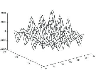
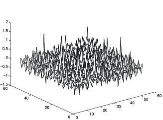
Figure 1: Multiscale representations for $x-p_{x}$ sections.

which corresponds to the full multiresolution expansion in all time scales. Formula (17) gives us expansion into a slow part $z_{N}^{slow}$ and fast oscillating parts for arbitrary N. So, we may move from coarse scales of resolution to the finest one for obtaining more detailed information about our dynamical process. The first term in the RHS of equation (19) corresponds on the global level of function space decomposition to resolution space and the second one to detail space. In this way we give contribution to our full solution from each scale of resolution or each time scale. On Fig. 1 we present sections $x-p_{x}$ corresponding to model (5) in different parameter regions.

4 ACKNOWLEDGMENTS

We would like to thank The U.S. Civilian Research & Development Foundation (CRDF) for support (Grants TGP-454, 455), which gave us the possibility to present our nine papers during PAC2001 Conference in Chicago and Ms. Camille de Walder from CRDF for her help and encouragement.

References

- [1] A.N. Fedorova and M.G. Zeitlin, Math. and Comp. in Simulation, 46, 527, 1998.
- [2] A.N. Fedorova and M.G. Zeitlin, New Applications of Nonlinear and Chaotic Dynamics in Mechanics, 31, 101 Kluwer, 1998.
-
[3]
A.N. Fedorova and M.G. Zeitlin,
CP405, 87, American Institute of Physics, 1997.
Los Alamos preprint, physics/9710035. - [4] A.N. Fedorova, M.G. Zeitlin and Z. Parsa, Proc. PAC97 2, 1502, 1505, 1508, APS/IEEE, 1998.
- [5] A.N. Fedorova, M.G. Zeitlin and Z. Parsa, Proc. EPAC98, 930, 933, Institute of Physics, 1998.
- [6] A.N. Fedorova, M.G. Zeitlin and Z. Parsa, CP468, 48, American Institute of Physics, 1999. Los Alamos preprint, physics/990262.
- [7] A.N. Fedorova, M.G. Zeitlin and Z. Parsa, CP468, 69, American Institute of Physics, 1999. Los Alamos preprint, physics/990263.
-
[8]
A.N. Fedorova and M.G. Zeitlin,
Proc. PAC99,
1614, 1617, 1620, 2900, 2903,
2906, 2909, 2912, APS/IEEE, New York, 1999.
Los Alamos preprints:
physics/9904039,
physics/9904040, physics/9904041, physics/9904042,
physics/9904043, physics/9904045, physics/9904046,
physics/9904047. - [9] A.N. Fedorova and M.G. Zeitlin, The Physics of High Brightness Beams, 235, World Scientific, 2000. Los Alamos preprint: physics/0003095.
-
[10]
A.N. Fedorova and M.G. Zeitlin, Proc. EPAC00, 415, 872, 1101, 1190, 1339, 2325,Austrian Acad.Sci.,2000.
Los Alamos preprints: physics/0008045, physics/0008046,
physics/0008047, physics/0008048, physics/0008049,
physics/0008050. - [11] A.N. Fedorova, M.G. Zeitlin, Proc. 20 International Linac Conf., 300, 303, SLAC, Stanford, 2000. Los Alamos preprints: physics/0008043, physics/0008200.
-
[12]
A.N. Fedorova, M.G. Zeitlin, Los Alamos preprints:
physics/0101006, physics/0101007 and World Scientific, in press. -
[13]
A. Dragt, Lectures on Nonlinear Dynamics, 1996.
A. Bazzarini, e.a., CERN 94-02. - [14] A. Cohen, e.a., CPAM, 45, 485, 1992