Statistics of Atmospheric Correlations

Abstract

For a large class of quantum systems the statistical properties of their spectrum show remarkable agreement with random matrix predictions. Recent advances show that the scope of random matrix theory is much wider. In this work, we show that the random matrix approach can be beneficially applied to a completely different classical domain, namely, to the empirical correlation matrices obtained from the analysis of the basic atmospheric parameters that characterise the state of atmosphere. We show that the spectrum of atmospheric correlation matrices satisfy the random matrix prescription. In particular, the eigenmodes of the atmospheric empirical correlation matrices that have physical significance are marked by deviations from the eigenvector distribution.

I Introduction

The study of random matrix ensembles have brought in a great deal of insight in several fields of physics ranging from nuclear, atomic and molecular physics, quantum chaos and mesoscopic systems [1]. The interest in random matrices arose from the need to understand the spectral properties of the many-body quantum systems with complex interactions. With general assumptions about the symmetry properties of the system dictated by quantum physics, random matrix theory (RMT) provides remarkably successful predictions for the statistical properties of the spectrum, which have been numerically and experimentally verified in the last few decades [2]. In recent times, it has been realised that the fluctuation properties of low-dimensional systems, e.g. chaotic quantum systems, are universal and can be modelled by an appropriate ensemble of random matrices [3]. From its origins in quantum physics of high dimensional systems, the scope of RMT is further widening with the new approaches based on supersymmetry methods [4] and applications in seemingly disparate fields like quantum chromodynamics [5], two-dimensional quantum gravity [6], conformal field theory [1] and even financial markets [7]. Thus, random matrix techniques have potential applications and utility in disciplines far outside of quantum physics. In this, we show that the empirical correlation matrices that arise in atmospheric sciences can also be modelled as a random matrix chosen from an appropriate ensemble.

The correlation studies are elegantly carried out in the matrix framework. The empirical correlation matrices arise in a multivariate setting in various disciplines; for instance, in the analysis of space-time data in general problems of image processing and pattern recognition, in particular for image compression and denoising [8]; the weather and climate data are frequently subjected to principal component analysis to identify the independent modes of atmospheric variability [9]; in the study of financial assets and portfolios through the Markowitz’s theory of optimal portfolios [10]. Most often, the analysis performed on the correlation matrices is aimed at separating the signal from ‘noise’, i.e. to cull the physically meaningful modes of the correlation matrix from the underlying noise. Several methods based on Monte-Carlo simulations have been used for this purpose [11]. The general premise of such methods is to simulate ’noise’ by constructing an ensemble of matrices with random entries drawn from specified distributions and the statistical properties of its eigenvalues, like the level density etc., are compared with that of the correlation matrices. Even as the Monte-Carlo techniques become computationally expensive beyond a point, asymptotic formulations take over. The deviations from ’pure noise’ assumptions are interpreted as signals or symptom of physical significance. In the context of the atmospheric sciences, empirical correlation matrices are widely used, for example, to study the large scale patterns of atmospheric variability. If the random matrix techniques are valid for a correlation matrix, it might be useful as a tool to separate the signal from the noise, with lesser computational expense than with methods based on Monte-Carlo techniques. We show that RMT prediction for eigenvector distribution has potential application in this direction for atmospheric correlation matrices.

II Correlations and Teleconnections

The state of the atmosphere is governed by the classical laws of fluid motion and exhibits a great deal of correlations in various spatial and temporal scales. These correlations are crucial to understand the short and long term trends in climate. Generally, atmospheric correlations can be recognised from the study of empirical correlation matrices constructed using the atmospheric data.

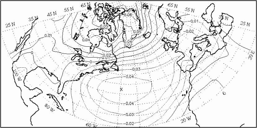
FIG. 1.: The NAO pattern as captured by the EOF analysis of sea-level pressure, with the geographical map of the domain of analysis in the background. The contours are drawn after averaging over the first two dominant EOFs. Note the north-south dipole shown as closed contours, in mid-Atlantic (dotted contour) and over Greenland (solid contours).

FIG. 2.: Dominant EOF from analysis of wind-stress vectors with the equatorial Pacific Ocean domain in the background. This eigenmode predominantly represents the annual fluctuations in trade winds and accounts for 38% of the variability. This eigenvector has been rotated by $45^{o}$ to obtain physically meaningful pattern.

Most significant correlations are documented as teleconnection patterns, i.e., the simultaneous correlations in the fluctuations of the large scale atmospheric parameters at widely separated points on the earth. They could be thought of as the dominant modes of atmospheric variability. Wallace and Gutzler have surveyed the entire northern hemisphere teleconnections and show that the dominant eigenmodes of the correlation matrices, in most cases, reflect these teleconnection patterns [12]. For instance, the North Atlantic Oscillation (NAO) [13] refers to the exchange of the atmospheric mass between Greenland/Iceland region and the regions of North Atlantic ocean between $35^{o}\mbox{N}$ and $40^{o}\mbox{N}$ and is characterised by a north-south dipole pattern as shown in Fig. 1. It is known that the NAO is associated with anomalous weather patterns in the eastern US and northern Europe including Scandinavia [14]. Such dominant modes need not always have to be a teleconnection. For example, the pattern in Fig 2 can be identified with the annual trade wind fluctuations in the equatorial Pacific region; obtained as a dominant eigenmode from the analysis of the pseudo wind stress vectors. In subsequent sections, we will perform statistical analysis on the spectra of atmospheric correlation matrices, whose dominant modes display correlation patterns discussed above. Atmospheric correlations are interesting to study from a RMT perspective because they arise naturally from known physical interactions and offers instances to verify two (orthogonal and unitary) of the three Gaussian ensembles of RMT.

A Empirical Orthogonal Functions

The Empirical Orthogonal Function (EOF) method, also called the Principal Component Analysis, is a multivariate statistical technique widely used in the analysis of geophysical data [9]. It is similar to the singular value decomposition employed in linear algebra and it provides information about the independent modes of variabilities exhibited by the system.

In general, any atmospheric parameter $z(x,t)$, (like wind velocity, geopotential height, temperature etc.), varies with space$(x)$ and time$(t)$ and is assumed to follow an average trend on which the variations (or anomalies, as referred to in atmospheric sciences) are superimposed, i.e., $z(x,t)=z_{avg}(x)+z^{\prime}(x,t)$. The wind vectors can be represented as a complex number, $se^{i\theta}$ where $s$ is the wind speed and $\theta$ the direction. Thus, in general, $z(x,t)$ could be a complex number. The mathematical treatment of complex correlations and EOFs is given in ref [15]. In further analysis, the standardised anomaly $z^{\prime}(x,t)$ will be used which will have zero mean ($\overline{z^{\prime}}(x)=0$) and is rescaled such that its variance $<z^{\prime}(x)^{2}>$ is unity. If the observations were taken $n$ times at each of the $p$ spatial locations and the corresponding anomalies $z^{\prime}(x,t)$ assembled in the data matrix Z of order $p$ by $n$, then the spatial correlation matrix of the anomalies is given by,

$$\mbox{\bf S}=\frac{1}{n}\;\mbox{\bf Z}\;\mbox{\bf Z}^{\dagger}$$ (1)

Note that the elements of the hermitian matrix S, of order $p$, are just the Pearson correlation between various spatial points. The eigenfunctions of S are called the empirical orthogonal functions since they form a complete set of orthogonal basis to represent the data matrix Z. In the geophysical setting, the EOFs can be plotted as contour maps by associating each component with its corresponding spatial location as shown in Fig 1. If the eigenvalue corresponding to the $m$th eigenmode is $\lambda_{m}$, then the percentage variance associated with the mode is given by, $v_{m}=(\lambda_{m}/\sum^{p}_{i=1}\lambda_{i})100.0.$ Then, the dominant mode would correspond to the EOF with the largest eigenvalue. In the last few decades, several variants of this basic EOF technique have been used to suit varied requirements [9]. We will show that the spectrum of S displays random matrix type spectral statistics.

III Eigenvalue statistics

A Data and analysis

Computing reliable correlation matrices depend on the availability of sufficiently long time series of data. Generally, the requirement is to have $n>>p$, as otherwise the computed covariances could be noisy and correlations could be regarded as random. Reliable records of monthly averages for weather and climate parameters of interest exist for the last 50 years. In our study, we use both the daily as well as the monthly averaged data available from NCEP reanalysis archives [16]. Further in this direction, we study three cases; (i) monthly mean sea level pressure (SLP) for the Atlantic domain $(0-90^{o}\mbox{N},120^{o}\mbox{W}-30^{o}\mbox{E})$ from 1948 to 1999. (ii) monthly mean global sea surface temperatures (SST) [17] and (iii) surface level pseudo wind-stress vectors in the equatorial Pacific ocean $(20^{o}\mbox{S}-20^{o}\mbox{N},130^{o}\mbox{E}-70^{o}\mbox{W})$. The first case identifies many northern hemisphere teleconnections and its climatic effects and EOF aspects are documented [12]. Wind-stress is an important quantity in studies on coupled ocean-atmosphere models that simulate the air-sea interaction and the feedback mechanism. The pseudo wind-stress is defined as $W=\sqrt{(u^{2}+v^{2})}(u+iv)$, where $u$ and $v$ are the zonal and meridional wind components, and this leads to complex correlation matrix. Its EOFs exhibit signatures of the mean annual signal and ElNino oscillations [18]. Note that the eigenmodes of complex correlation matrix are determined only up to a complex factor of unit modulus. This allows the freedom to choose a phase angle to rotate the eigenvectors.

The atmospheric data is on an uniform spatial grid of $2.5^{o}$ along both the latitude and longitude. To ensure that $n>p$, in the calculations with monthly mean data, the spatial resolution was reduced to $5^{o}$. Thus, for the case(i) of monthly mean SLP correlations, p=434 and n=624. In the case (iii) of monthly mean wind stress analysis over equatorial Pacific ocean, the land points were removed from the calculations using land-sea mask and it results in p=494 and n=624. Since a longer time-series of monthly mean data was not available, another experiment was performed with daily averaged time-series from 1990 to 1999 with much improved ratio for $r=n/p$ in the range 2.5-3.5. The required means and anomalies were computed from which matrices of orders ranging from 500 to 1200 is constructed and diagonalised using standard LAPACK routines [19].

FIG. 3.: The integrated level density, in the form of a staircase, for the eigenvalues of the monthly mean SLP correlation matrix. The solid line is the empirical curve that fits the level density with dark circles denoting the location of eigenvalues. The inset is magnified view of a part of the curve.

First we look at the structure of eigenvalue density. The integrated level density $N(\lambda)=\sum\Theta(\lambda-\lambda_{i})$, can be written as, $N(\lambda)\approx N_{avg}(\lambda)+N_{fl}(\lambda)$, a sum of an average part and the fluctuating part. The eigenvalues $\lambda_{i}$ are unfolded by fitting an empirical function to the average part of the integrated level density such that the unfolded eigenvalues $\epsilon_{i}=N_{avg}(\lambda_{i})$ have mean spacing unity [20]. All the analysis reported further were performed on $\epsilon_{i}$. As Fig. 3 shows, for empirical correlation matrices, the spectrum is dense at the lower end. This is typical of the spectrum of correlation matrices formed from the data matrix Z through eq (1) [21]. In contrast to this, for a generic quantum system, the level density increases with energy and is dense at the higher end of the spectrum.

B Level spacing distribution

One of the celebrated results of the random matrix theory is the nearest-neighbour eigenvalue spacing distribution; i.e. the distribution of $s_{i}=\epsilon_{i+1}-\epsilon_{i}$. It gives the probability for finding the neighbouring levels with a given spacing $s$. In the context of this work, the Gaussian Orthogonal Ensemble (GOE) is appropriate for the mean sea-level pressure correlations and Gaussian Unitary Ensemble (GUE) for pseudo wind-stress vectors. The spectra of these classes exhibit universal fluctuation properties and the spacing distributions are given by [22],

$$P_{\mbox{GOE}}(s) = \frac{\pi}{2}\;s\exp(-\frac{\pi}{4}s^{2})$$ (2)

$$P_{\mbox{GUE}}(s) = \frac{32}{\pi^{2}}\;s^{2}\exp(-\frac{4}{\pi}s^{2})$$ (3)

The analytical forms above indicate level-repulsion, a tendency against clustering, as evident from low probability for small spacings. The level repulsion is linear for GOE and quadratic for GUE.

FIG. 4.: Eigenvalue spacing distribution for the monthly mean SLP correlation matrix. The solid curve is the GOE prediction. The inset shows the cumulative distribution for the monthly and daily averaged correlation matrix.

In Fig. 4, we show the spacing distribution for the eigenvalues of the correlation matrix of the monthly mean SLP. The inset in this figure shows the cumulative spacing distribution for the spectra obtained from the analysis of monthly and daily averaged SLP data. We observe a general agreement with the RMT predictions. In Fig. 5, the spectra from the monthly mean wind-stress correlation data is shown. If the spacings, $s$, were uncorrelated then we would expect a Poisson distribution, $P(s)=\exp(-s)$ [20]. In all the cases we studied, the empirical histograms do not follow the Poisson curves at all. As would be expected, a better agreement between the theoretical curves and the empirical distributions is observed in the analysis of daily averaged data, in both the cases of SLP and pseudo wind-stress correlations, since they provide about 1000 eigenvalues for the statistics. For instance, a Kolmogrov-Smirnov test at 65% confidence level could not reject the hypothesis that GOE is the correct distribution for the eigenvalues of monthly mean SLP correlation matrix, whereas a similar test for the daily averaged SLP data could not reject the hypothesis at 99% confidence level. The monthly mean SST correlation matrix analysis (not shown here) also supports RMT spacing distribution. The eigenvalue spacing distribution for the equatorial Pacific pseudo wind-stress vector correlation matrix also indicates a good agreement with the GUE prediction given by Eq (3) (see Fig 5).

FIG. 5.: Eigenvalue spacing distribution for the monthly mean wind-stress correlation matrix. The solid curve is the GUE prediction. The inset shows the cumulative distribution for the monthly and daily averaged correlation matrix.

C Long-range Correlations

Beyond the nearest-neighbour spacing distribution, we study the long-range correlations. We compute the following spectral fluctuation measures [20] which are based on the two-point correlation function. (a) The spectral rigidity, the so-called $\Delta_{3}$ statistic, measures the least-square deviation of the spectral staircase function $N(\epsilon)$ from the straight line of best fit for a finite interval $L$ of the spectrum,

$$\Delta_{3}(L,L^{\prime})=\frac{1}{L}\stackrel{{\scriptstyle\mbox{min}}}{{a,b}}\int^{L^{\prime}+L}_{L^{\prime}}[N(\epsilon)-a\epsilon-b]^{2}\;\;d\epsilon$$ (4)

where $a$ and $b$ are obtained from a least-squares fit. Average over several choices of $L^{\prime}$ gives the spectral rigidity $\Delta_{3}(L)$. (b) the number variance $\Sigma^{2}$ is also a function of two-point correlation function. Let $n(L,L^{\prime})$ be the number of eigenvalues in the spectral interval $L$. Then, for a choice of $L^{\prime}$, $\Sigma^{2}$ is given by,

$$\Sigma^{2}(L,L^{\prime})=n(L,L^{\prime})^{2}-L^{2}$$ (5)

Averaging $n(L,L^{\prime})^{2}$ over $L^{\prime}$ gives the number variance $\Sigma^{2}(L)$. The asymptotic results, for large $L$, from random matrix considerations, is given by [22],

$$\Delta_{3}(L) = \frac{1}{\nu\pi^{2}}\log(L)+g_{\nu}$$ (6)

$$\Sigma^{2}(L) = \frac{2}{\nu\pi^{2}}\log(L)+h_{\nu}$$ (7)

where $\nu=1,2$ corresponds to GOE and GUE respectively; $g$ and $h$ are also dependent on the ensemble.

FIG. 6.: $\Delta_{3}(L)$ for spectra from the correlation matrix of (a) wind stress and (b) SLP. The solid curve in (a) is GUE prediction and in (b) the GOE prediction. The circles are for the correlation matrix obtained from daily averaged data and triangles represent the matrix obtained from the monthly mean data.

Fig 6 shows the $\Delta_{3}(L)$ statistic for the SLP and wind-stress correlation matrix spectrum, computed using the method given by Bohigas and Giannoni [20]. Generally, a good agreement is observed with the RMT predictions. In all the cases, for small $L$ the agreement is good and small deviations begin to be seen for larger values indicating a possible breakdown of universality. In general, this should indicate system specific features that cannot be modelled by assumptions based on randomness. Once again, we notice that the correlation matrix spectra obtained from daily data show better agreement with RMT predictions, primarily due to larger orders of correlation matrix involved and hence more eigenvalues for the analysis. Fig 7 shows the number variance $\Sigma^{2}(L)$ for all the cases. We observe a fairly good agreement with RMT predictions. The results for SLP and SST correlations are in broad agreement with the similar analysis performed on the financial correlation matrices [7], both of which are modelled by the orthogonal ensemble of RMT. This, in itself, demonstrates the breadth of applications of RMT.

FIG. 7.: $\Sigma^{2}(L)$ for spectra from the correlation matrix of (a) wind stress and (b) SLP. The circles are for the correlation matrix obtained from daily averaged data and triangles represent the matrix obtained from the monthly mean data.

IV Statistics of EOF components

With the eigenvalue statistics, it is not straightforward to obtain detailed system specific information, unless there are significant deviations from random matrix predictions. The distribution of eigenvector components, on the other hand, reveals fine-grained information, at the level of every eigenvector. In this section, we show that almost all the EOFs follow the RMT distribution. However, a few EOFs that have physical significance, like the ones shown in Figs 1 and 2, deviate strongly from RMT. Broadly, the variability captured by an EOF is seen to be reflected in its deviation from RMT predictions.

Let $a^{m}_{j}$ be the $j$th component of the $m$th eigenvector. Assuming that these components are Gaussian random variables with the norm being their only characteristic, it can be shown that the distribution of $r=|a^{m}_{j}|^{2}$, in the limit when the matrix dimension is large, is given by the special cases of the $\chi^{2}$ distribution [23],

$$P_{\nu}(r)=\left(\frac{\nu}{2<r>}\right)^{\nu/2}\;\frac{r^{\nu/2-1}}{\Gamma(\frac{\nu}{2})}\;\exp\left(\frac{-r\nu}{2<r>}\right)$$ (8)

The case $\nu=1$ can be identified with GOE and gives the well-known Porter-Thomas (PT) distribution. The distribution of complex eigenvectors correspond to GUE class with $\nu=2$. The general understanding is that if the eigenvectors are sufficiently irregular in some sense, then its components are $\chi^{2}$ distributed and deviations occur if they show some symptoms of regularity.

FIG. 8.: Cumulative distribution of EOF components for the SLP correlation matrix. The solid curve is the Porter-Thomas distribution. The two curves with dotted lines correspond to the first two dominant EOFs, whose spatial map is shown in Fig. 1. The long-dashed curves are the next few dominant EOFs. The curve with dark-circles is a sample from the bulk of lesser-dominant EOFs that mostly follow Porter-Thomas distribution. The curve with small dashes (marked as 45) is the 45th EOF that surprisingly deviates from the PT curve (see text).

In further analysis, we will use the modulus square of the EOF components, i.e. $r=|a^{m}_{j}|^{2}$, normalised to unit mean. For the monthly mean SLP correlation matrix, Fig 8 shows the cumulative distribution of EOF components. Since EOFs form an optimal basis to represent the data, most of the variability is carried by a small number of EOFs; in this case about 91% of the variability is captured by just 12 dominant EOFs. The rest 9% is accounted for by the bulk of the rest 422 EOFs. The central result of this section is that the bulk of these EOFs, accounting for a small fraction of the variability, follow the cumulative Porter-Thomas (PT) distribution given by, $I(r)=\mbox{erf}(\sqrt{r/2})$, where erf is the standard error function. This strengthens the conclusion that the empirical correlation matrices can be modelled as a random matrix. As an example from a large number of such EOFs, the distribution of 294th EOF is shown (denoted by dark circles) in Fig 8, and it practically falls on the PT curve. We observed that the distribution of the all such EOFs follow RMT and this is also confirmed by a Kolmogrov-Smirnov test.

FIG. 9.: Cumulative distribution of EOF components for the pseudo wind-stress correlations. The solid curve is the GUE prediction. The dotted curves are for the first two dominant EOFs; the spatial map of dominant EOF shown in Fig. 2. The curve with dark-circles is a sample from the bulk of lesser-dominant EOFs that follow GUE. The curve with small dashes (marked as 4) is the 4th EOF deviates significantly from the GUE prediction.

However, interesting cases arise from a small number of dominant EOFs which deviate strongly from RMT predictions. The first two dominant EOFs shown in Fig 8 (as dotted lines), representing about 30% and 22% of the entire variability, show significant deviations from cumulative PT curve. The spatial structure of both these eigenmodes, shown in Fig 1, jointly capture the essence of North-Atlantic pattern. This scenario, of most dominant of the EOFs deviating from the PT distribution and lesser significant ones showing agreement with it, is repeated in the analysis of SST (not shown here) and daily averaged SLP correlations as well. At this point, we stress that these deviations are exceptions that arise in about 1% of the EOFs.

Fig 9 shows the cumulative distribution for the EOFs obtained from the analysis of the monthly mean wind-stress correlation. Note that in this case, the appropriate prediction follows the unitary ensemble since the EOF components are complex. The dominant 20 EOFs explain nearly 90% of the variability in the wind stress data. The rest of the large number (about 400) of EOFs show good agreement with cumulative GUE curve for eigenvector distribution given by $I(r)=1-\exp(-r)$. One such case, 370th EOF, is shown in Fig 9 denoted by dark circles. In general, EOFs show good agreement with RMT except for the few dominant EOFs. The dominant EOF, whose spatial pattern is shown in Fig 2, represents the mean annual Pacific trade-wind fluctuations and explains 38% of the variability and shows pronounced deviation from the cumulative GUE curve. Next few dominant EOFs also exhibit significant deviations. Legler [18] has performed EOF analysis on the Pacific ocean wind-stress vectors and attributed physical significance to the top three dominant EOFs. Thus, EOFs that have physical significance, cannot be modelled by RMT ensembles. An analogy with quantum eigenstates seems inevitable. Studies on the distribution of the eigenfunctions of low-disorder tight-binding systems and chaotic quantum systems show that a small fraction of the eigenstates, which display quantum localisation, deviate from random matrix predictions [24], while most others show RMT-like behaviour.

There are two interesting observations in this study. Firstly, we notice that there are few EOFs, occurring at irregular intervals, which do not carry much of a significance in terms of the variability but deviate strongly from RMT predictions. It is not immediately clear if they carry any significant information. Secondly, a surprising observation is that the EOFs, corresponding to first few eigenvalues at the lower end of the spectrum, most often regarded as least dominant and random, devoid of any system specific information, show marked deviations from RMT (see also ref [7]). One such example for each of GOE and GUE case is shown in Figs 8 and 9.

V Discussion and conclusion

This work shows that the random matrix predictions are of considerable interest in the study of the correlation matrices that arise in atmospheric sciences. Previous work on the correlations of stock market fluctuations has come to similar conclusion [7]. This is despite the following basic difference; RMT assumes that the quantum Hamiltonian matrix is part of an ensemble of random matrices whose entries are independent random numbers drawn from a Gaussian distribution. In the correlation matrix formalism, the elements of data matrix are independent Gaussian distributed random numbers. Then, the correlation matrix in eq. 1 follows Wishart structure [25], a form of generalised $\chi^{2}$-distribution.

In the application of EOFs in various disciplines an important question is the truncation of EOFs while opting for a low-dimensional representation for a given data matrix. The earlier approaches to this problem were based on Monte-Carlo techniques or asymptotic theories [9, 11]. It would be interesting to evolve a truncation criteria, for using EOFs as empirical basis, from random matrix techniques since the results here suggest that RMT could be potentially applied to separate the random modes from the physically significant modes of the correlation matrix.

Even as we have documented evidence for RMT like behaviour from the atmospheric correlation matrices, there is also a need to look at the limits of RMT description. For instance, a correlation matrix which shows perfect correlation will obviously not behave like RMT. Can correlation matrix spectra display Poisson spacing distribution ? Such limits of RMT in the context of correlation matrix is yet to be explored.

In summary, we have analysed atmospheric correlation matrices from the perspective of random matrix theory. The central result of this work is that they can be modelled as random matrices chosen from an appropriate RMT ensemble. The eigenvalue statistics exhibits short and long-range RMT-type behaviour. Most of the eigenmodes also follow the RMT type eigenvector distribution. Few dominant eigenmodes that have physical significance deviate from RMT predictions. We have verified our conclusions with examples of correlation matrices that belong to GOE and GUE universality classes of random matrix theory.

REFERENCES

- [1] T. Guhr, A. Muller-Groeling and H. A. Weidenmuller, Phys. Rep. 299 189 (1999).
- [2] T. Zimmermann et. al., Phys. Rev. Lett. 61 3 (1988); A. Kudrolli et. al., Phys. Rev. E 49 R11 (1994)
- [3] O. Bohigas, M. J. Giannoni and C. Schmidt, Phys. Rev. Lett. 52 1 (1984).
- [4] K. Efetov, Supersymmetry in Disorder and Chaos (Cambridge Univ. Press, 1997).
- [5] J.J.M. Verbaarschot, Nucl. Phys. B (Proc. Suppl.) 53 88 (1997).
- [6] E. Abdalla, Lecture Notes in Physics 20 (Springer,Berlin, 1994).
- [7] L. Laloux et. al., Phys. Rev. Lett. 83 1467 (1999); V. Plerou et. al., Phys. Rev. Lett. 83 1471 (1999).
- [8] R. N. Hoffman and D. W. Johnson, IEEE Trans. Geosci. Remote Sensing 32 25 (1994) and references therein.
- [9] R. W. Preisendorfer, (ed. C. D. Mobley) Principal Component Analysis in Meteorology and Oceanography, (Elsevier,1988); Daniel S. Wilks, Statistical Methods in Atmospheric Sciences (Academic Press, London, 1995).
- [10] E. J. Elton and M. J. Gruber, Modern Portfolio Theory and Investment Analysis (John Wiley, New York, 1995) ; H. Markowitz, Portfolio Selection : Efficient Diversification of Investments (John Wiley, New York, 1959)
- [11] R. W. Preisendorfer, F. W. Zweirs and T. P. Barnett, Foundations of Principal Component Selection Rules, Scripps Inst. of Oceanography, SIO Ref. Series 81-4 (NTIS PB83-146613).
- [12] J. M. Wallace and Gutzler, Mon. Wea. Rev. 109 784 (1981).
- [13] P. J. Lamb and R. A. Peppler, Bull. Am. Met. Soc. 68 1218 (1987); H. van Loon and J. C. Rogers, Mon. Wea. Rev. 106 296 (1978); J. C. Rogers, Mon. Wea. Rev. 112 1999 (1984).
- [14] J. W. Hurrell, Science 269 676 (1995).
- [15] D. M. Hardy and J.J. Walton, J. Appl. Met. 17 1153 (1978).
- [16] The data is taken from the NCEP 50-year reanalysis archives of NOAA-CIRES at http://www.cdc.noaa.gov. The daily and monthly mean data and its derivatives are available from 1948 onwards.
- [17] T. M. Smith et. al., J. Clim. 9 1403 (1996).
- [18] D. M. Legler, Bull. Am. Met. Soc. 64 234 (1983).
- [19] http://www.netlib.org/lapack
- [20] O. Bohigas and M.-J. Giannoni in Mathematical and Computational Methods in Nuclear Physics, Vol 209 of Lecture Notes in Physics, edited by J. S. Dehesa, J. M. G. Gomez and A. Polls (Springer, 1984).
- [21] A. M. Sengupta and P. P. Mitra, Phys. Rev. E 60 3389 (1999).
- [22] M. L. Mehta, Random Matrices Academic Press, (1991).
- [23] F. Haake, Quantum Signatures of Chaos (Springer-Verlag, 1991).
- [24] K. Muller et. al., Phys. Rev. Lett. 78 215 (1997).
- [25] S. S. Wilks, Mathematical Statistics (John Wiley, New York, 1962).