[

Generation of Bright Soliton through the Interaction of Black Solitons

Abstract

We report on the possibility of having two black solitons interacting inside a silica fiber that presents normal group-velocity dispersion, to generate a pair of solitons, a vector soliton of the black-bright type. The model obeys a pair of coupled nonlinear Schrödinger equations, that follows in accordance with a Ginzburg-Landau equation describing the anisotropic $XY$ model. We solve the coupled equations using a trial-orbit method, which plays a significant role when the Schrödinger equations are reduced to first order differential equations.

PACS numbers: 05.45.Yv, 42.81.Dp, 11.27.+d

]

Solitary waves and solitons are relevant to a variety of nonlinear physical processes. They have made perhaps the geatest experimental impact in the field of nonlinear fiber optics, which are widely known to support solitons of several different types [1, 2, 3]. For instance, in silica fibers there are optical solitons of the bright and dark types. They appear because the Kerr nonlinearity in silica is always described by a positive coefficient, so that the sign of the group-velocity dispersion distinguishes two different types of solitons in silica fibers: the bright soliton, for negative sign of the group-velocity dispersion, and the dark soliton, for positive group-velocity dispersion. These two types of optical solitons were first reported in Ref. [4], in the case of bright solitons, and in Ref. [5], in the case of dark solitons. They are solutions of the cubic nonlinear Schrödinger equation, and they are characterized by having distinct profile: the bright soliton has vanishing asymptotic behavior, so they engender trivial topological behavior. On the other hand, dark solitons are characterized by non vanishing asymptotic behavior, so the presence of topological profile is one important feature of dark solitons. The central characteristic of dark solitons is the presence of a dip in its center, which distinguishes two possibilities: black solitons, in the case the dip reaches the botton, that is, if the dip goes completely to zero, and gray solitons, in the other cases.

Although both bright and dark solitons are widely known to be present in fibers, they are not exclusive of fibers. They can also appear in other systems, in particular in Bose-Einstein condensates (BEC), and in magnetic materials. The old prediction that an ideal gas of identical bosons may condensate into a macroscopic quantum state has recently been accomplished: BECs of different atomic elements were first produced in [6, 7, 8], and are reviewed for instance in Ref. [9]. Soom after this achievment, the presence of bright solitons in a BEC was first reported in Ref.[10], in the study of the dynamics of ultracold bosonic atoms loaded in an optical lattice, that is, in a lattice induced by the interference of an array of laser beams [11]. The presence of dark solitons was reported more recently in Refs. [12, 13]. The presence of bright or dark solitons in BEC is directly related to the physics of attractive or repulsive atomic interaction, respectivelly, in a mean-field description that follows in accordance with the Gross-Pitaevskii equation [14]. In magnetic films one finds dark solitons [15, 16, 17] in the form of a microwave magnetic envelope (MME). A good example of this was recently reported in Ref. [18], where one can find an interesting way of generating dark MME solitons, which opens a new route for the investigation of dark solitons in magnetic systems.

In silica fibers both black and bright solitons spring as solutions of the cubic non-linear Schrödinger equation, with just a change in the sign of the term that controls the group-velocity dispersion in that equation. We illustrate the two possibilities considering the normalized equation that describes the electric field envelope $U=U(x,z)$ inside the optical fiber

$$i\frac{\partial U_{\pm}}{\partial z}\pm\frac{1}{2}\frac{\partial^{2}U_{\pm}}{\partial x^{2}}+|U_{\pm}|^{2}U_{\pm}=0$$ (1)

The variables $x$ and $z$ describe the reduced time and space coordinates inside the fiber, respectively. This equation takes into accound the temporal or group-velocity dispersion, the second term in the above Schrödinger equation, and weak Kerr nonlinearity, the third term in Eq. (1). The two signs represent the two standard situations, that generate the black and bright solitons.

The presence of solitons follows after writing $U_{\pm}(x,t)=u_{\pm}(x)exp(iz)$. We get

$$\frac{1}{2}\frac{d^{2}u_{\pm}}{dx^{2}}=\pm\,u_{\pm}\mp u^{3}_{\pm}$$ (2)

These equations are solved by

$$u_{+}(x) = \pm{\rm sech}(x-{\bar{x}})$$ (3)

$$u_{-}(x) = \pm\tanh(x-{\bar{x}})$$ (4)

where ${\bar{x}}$ is an arbitrary point, standing for the center of the soliton. Here $u_{+}(x)$ and $u_{-}(x)$ represent the fundamental solitons, the bright and dark solitons, respectively. In fact, $u_{-}(x)$ is a black soliton since the dip in $u^{2}_{-}(x)$ goes to zero, reaching the botton of the electric field envelope.

We consider the possibility of describing a more general situation. We think of using a single fiber, an optical medium with normal group-velocity dispersion. However, we illuminate the fiber with two distinct laser beams, having different amplitudes and opposite circular polarizations. The electric fields are characterized by the envelopes $U(x,z)$ and $V(x,z)$, and the system is described by the two normalized equations

$$i\frac{\partial U}{\partial z}-\frac{1}{2}\frac{\partial^{2}U}{\partial x^{2}}+F(I)U = 0$$ (5)

$$i\frac{\partial V}{\partial z}-\frac{1}{2}\frac{\partial^{2}V}{\partial x^{2}}+G(I)V = 0$$ (6)

We use $I=|U|^{2}+|V|^{2}$ to describe the total intensity inside the fiber, and now the envelopes of two interacting laser beams inside the optical medium are characterized by the functions $F(I)$ and $G(I)$, which respond to nonlinear Kerr interactions inside the silica fiber.

We describe the case of two different laser beams, that interact inside the silica fiber with the envelope of the electric fields in the form

$$U(x,z) = u(x)\;e^{iz}$$ (7)

$$V(x,z) = v(x)\;e^{irz}$$ (8)

Here $r$ is real and positive, and parametrizes the relative propagation constant of the vector constituents. We substitute Eqs. (7) and (8) into Eqs.(5) and (6) to obtain

$$\frac{1}{2}\frac{d^{2}u}{dx^{2}} = -u+F_{r}(u,v)\;u$$ (9)

$$\frac{1}{2}\frac{d^{2}v}{dx^{2}} = -r\;v+G_{r}(u,v)\;v$$ (10)

We normalize the system in a way such that, in the absence of $v$ we get $F_{r}(u,0)=u^{2}$, and in the absence of $u$ we get $G_{r}(0,v)=r^{2}v^{2}$. In the first case, for $v=0$ we get

$$\frac{1}{2}\frac{d^{2}u}{dx^{2}}=-u+u^{3}$$ (11)

whose solutions are

$$u_{b}(x)=\pm\tanh\left({x-{\bar{x}}}\right)$$ (12)

The second case is similar, leading to

$$v_{b}(x)=\pm\sqrt{\frac{1}{r}}\tanh[\sqrt{r}\,(x-{\bar{x}})]$$ (13)

These solutions represent black soliton solutions. The system we are preparing is such that in the reduced case of just one component, obtained after turning off one of the two laser beams, the interactions between the optical fiber and the beam give rise to a black soliton. Each one of the black solitons has its own characteristics, which are naturally related to each one of the two laser beams since we are not changing the optical medium, the fiber. The individual black solitons are different, giving rise to an asymmetrical arrangement that will allow interesting novelties. The idea is similar to those in Refs. [19, 20, 21], and the results remind us of other effects: in quantum optics, a superposition of two (antisqueezed) number states may exhibit squeezing effect [22], a property not shown by any isolated component; also, a superposition of two (most classical) coherent states may result in a nonclassical (Schrödinger’s cat) state, as observed experimentally for light fields [23] and for trapped ions [24].

The main characteristics of the two black solitons are depicted in Fig. 1, where we plot both the $u_{b}(x)$ and $v_{b}(x)$. We notice that the amplitude ($a$) and width ($w$) of $u_{b}(x)$ are such that $a_{u}=w_{u}=1$, but for $v_{b}(x)$ they become $a_{v}=w_{v}=\sqrt{1/r}$. Thus, in the following we will consider the case $r\in(0,1)$.

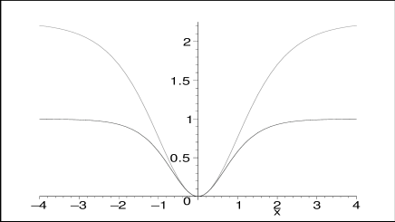
FIG. 1.: The two black solitons, $u^{2}_{b}(x)$ and $v^{2}_{b}(x)$, represented by thicker and thinner lines, respectively. They appear inside the optical fiber when one of the two laser beams is turned off. We use $r=4/9$.

The limit $r\to 1$ describes the case of interactions between laser beams of same amplitude but opposite circular polarizations in an isotropic Kerr medium. This case is simpler, and can be described by a system of symmetrically coupled nonlinear Schrödinger equations. For the pair of symmetrically coupled equations, if we set $F_{1}(u,v)=G_{1}(u,v)=u^{2}+v^{2}$ we get the well known Manakov model [25]. This model can also be used to represent the isotropic $XY$ model [26], which obeys the Ginzburg-Landau equation ${\partial A}/{\partial t}={\partial^{2}A}/{\partial x^{2}}+A-|A|^{2}A$, where $A$ is complex. We use $A=X+iY$ to show that for static configurations the above Ginzburg-Landau equation leads to the symmetrically coupled nonlinear Schrödinger equations. We use this as a guide toward the more general asymmetric model, and we consider the anisotropic $XY$ model, which is described by

$$\frac{\partial A}{\partial t}=\frac{\partial^{2}A}{\partial x^{2}}+A-|A|^{2}A+\alpha{\bar{A}}$$ (14)

where $\alpha$ is real. We use this model to investigate the case of two laser beams, in a medium such that $F_{r}(u,v)=u^{2}+r(2r+1)v^{2}$ and $G_{r}(u,v)=r^{2}v^{2}+r(2r+1)u^{2}$, that obey $F_{r}(u,0)=u^{2}$ and $G_{r}(0,v)=r^{2}\,v^{2}$, as required to recuperate the case describing a single laser beam, when the other beam is turned off. The form of the interaction is dictated by the anisotropic $XY$ model, and by the two laser beams that enter the fiber.

The above considerations settle the problem. And now the key issue follows after recognizing that the coupled Schrödinger equations can be seen as equations of motion for static fields that appear in models of two real scalar fields in bidimensional space-time [27]. In the case under examination the system of two fields is described by the potential

$$V(u,v)=\frac{1}{2}\left(-1+u^{2}+r\,v^{2}\right)^{2}+\frac{1}{2}\left(2r\,u\,v\right)^{2}$$ (15)

This potential has the general form [28, 29, 30]

$$V(u,v)=\frac{1}{2}\left(\frac{dW}{du}\right)^{2}+\frac{1}{2}\left(\frac{dW}{dv}\right)^{2}$$ (16)

where $W=W(u,v)$ is given by

$$W(u,v)=-u+\frac{1}{3}u^{3}+ruv^{2}$$ (17)

The pair of second order equations now become

$$\frac{1}{2}\frac{d^{2}u}{dx^{2}} = -u+u^{3}+r(2r+1)uv^{2}$$ (18)

$$\frac{1}{2}\frac{d^{2}v}{dx^{2}} = -rv+r^{2}v^{3}+r(2r+1)u^{2}v$$ (19)

The main issue here is that the above system of nonlinear Schrödinger equations can be solved exactly. There are two trivial solutions, that appear when one turns off one of the two beams. They are the fundamental black solitons $u_{1}(x)=u_{b}(x),\;v_{1}=0$ and $u_{2}=0,\;v_{2}(x)=v_{b}(x)$, which reproduce the former solutions (12) and (13). Furthermore, we also have the non-trivial vector soliton, described by

$$u_{2}(x) = \pm\tanh[{2r}(x-{\bar{x}})]$$ (20)

$$v_{2}(x) = \pm\sqrt{1/r-2\,}\;{\rm sech}[{2r}(x-{\bar{x}})]$$ (21)

This result is very interesting: it shows that two black solitons in interaction inside the silica fiber generate a pair of solitons, one of the black type and the other of the bright type. In Fig. 2 we depict this non-trivial vector soliton. It illustrate that the presence of bright solitons is not a privilege of specific fibers, that have anomalous group-velocity dispersion. We may say that the second laser beam sees the normal group-velocity dispersion of the medium as an anomalous one, and this appear through the presence of the first laser beam, which is responsible for changing the group-velocity dispersion inside the fiber. This phenomenon is new, and follows from the vector soliton (20) and (21). We notice that the vector soliton only exists for $r\in(0,1/2)$, and the limit $r\to 1/2$ leads us back to the scalar soliton $u_{b}(x)$. This model has the property that the limit $r\to 1$ is trivial. This limit leads to the symmetric situation, which can be investigated after rotating the the $(u,v)$ plane to $(u_{+},u_{-})$, with $u_{\pm}=u\pm v$. These transformations factorate the two-field system into two degenerate systems of a single field, that support no vector field solutions of the black and bright type. This shows that our model is asymmetric by construction, and the limit $r\to 1$ leads to a trivial symmetric model.

The presence of the nontrivial black-bright vector soliton is easier to see if we integrate the coupled equations (18) and (19) once. This gives the first order equations

$$\frac{du}{dx} = \mp 1\pm u^{2}\pm rv^{2}$$ (22)

$$\frac{dv}{dx} = \pm 2ruv$$ (23)

The fact that the pair of second order equations (18) and (19) can be integrated to give the above pair of first order equations (22) and (23) is fundamental, since it is easier to integrate. In Field Theory this identifies the Bogomol’nyi-Prasad-Sommerfield bound [31]; the solutions are stable and minimize the energy of the system [28, 29].

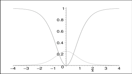
FIG. 2.: The black ($u^{2}_{2}(x)$, thicker line) and bright ($v^{2}_{2}(x)$, thinner line) solitons that appear inside the optical fiber when both the laser beams are turned on. We use $r=4/9$.

We solve the first order equations using the trial orbit method introduced in Ref. [32]. We try the orbit $u^{2}+av^{2}=1$, for $a$ being some real constant. We differentiate this expression and we use the first order equations (22) and (23) to obtain $u^{2}+r(1+2a)v^{2}=1$. This is compatible with the previous choice if and only if $a=r/(1-2r)$. Thus the orbit is given by

$$u^{2}+\frac{1}{\frac{1}{r}-2}\,v^{2}=1$$ (24)

It is an elliptical arc, that goes from $(u=\pm 1,v=0)$ to $(u=\mp 1,v=0)$ when $x$ spans the entire real line.

We use the orbit (24) to write the first order Eq. (22) in the form ${du}/{dx}=\mp 2r(1-u^{2})$. It can be integrated easily. The result gives the solution (20). The other solution (21) is obtained immediately from the orbit (24) obeyed by $u$ and $v$.

We have found the vector soliton as a solution of the pair of first order equations (22) and (23). The approach is new, and involves two steps: the first consists in transforming the pair of second order Schrödinger equations (18) and (19) into a pair of first order differential equations; the second step deals with the trial orbit method introduced in Ref. [32]. The trial orbit method was introduced to help solving second order equations of motion for relativistic systems of coupled scalar fields. In the present context, the effectiveness of the trial orbit method is direct, since we can use the first order equations themselves to check if the orbit we trial is good, that is, if the trial orbit does not contradict the first order equations that follow from the equations of motions. This check is immediate, and provides a direct trial for the eligibility of the orbit under investigation. This fact does not appear in the original proposal in Ref. [32], since there it deals with second order differential equations.

We see that when the potential is written in terms of $W(u,v)$, in the form (16), the two equations of motion are written as

$$\frac{d^{2}u}{dx^{2}} = W_{u}W_{uu}+W_{v}W_{vu}$$ (25)

$$\frac{d^{2}v}{dx^{2}} = W_{u}W_{uv}+W_{v}W_{vv}$$ (26)

where $W_{u}=\partial W/\partial u$, etc. We associate to these equations the pair of first order equations

$$\frac{du}{dx}=W_{u},\;\;\;\;\;\frac{dv}{dx}=W_{v}$$ (27)

We differentiate these first order equations to see that their solutions also solve the equations of motion. Thus, we can concentrate on the simpler task of solving first order equations to get solutions to the second order equations. This is an important advantage, but it is restricted to work when the composite vector soliton presents nontrivial topological feature, as happens with dark solitons. This is not the case for bright solitons, that engender trivial topological behavior. Thus we may wander if it is possible to use two bright solitons to generate a composite, bright-black vector soliton. Because the bright solitons are nontopological they cannot appear as solutions of first order equations, as recently shown in Ref. [33].

We thank A. F. Lima and P. C. Oliveira for discussions, and CAPES, CNPq, and PRONEX for partial support.

REFERENCES

- [1] G. P. Agrawal, Nonlinear Fiber Optics (Academic, San Diego, 1995).
- [2] M. Hasegawa and Y. Kodama, Solitons in Optical Communications (Oxford University Press, Oxford, 1995).
- [3] Y. S. Kivshar and B. Luther-Davies, Phys. Rep. 298, 81 (1998).
- [4] I.F. Mollenauer, R.H. Stolen, and Gordon, Phys. Rev. Lett. 45, 1095 (1980).
- [5] Ph. Emplit et al., Opt. Commun. 62, 374 (1987); D. Krökel et al., Phys. Rev. Lett. 60, 29 (1988); A.M. Werner et al., Phys. Rev. Lett. 61, 2445 (1988).
- [6] M. H. Anderson et al. Science 269, 198 (1995).
- [7] K. B. Davis et al. Phys. Rev. Lett. 75, 3969 (1995).
- [8] C. C. Dradley, C. A. Sackett, R. G. Hulet, Phys. Rev. Lett. 78, 985 (1997).
- [9] A. S. Parkins and D. F. Walls, Phys. Rep. 303, 1 (1998).
- [10] D. Jaksch et al., Phys. Rev. Lett. 81, 3108 (1998).
- [11] G. Raithel et al., Phys. Rev. Lett. 78, 630 (1997); T. Müller-Seydlitz et al., Phys. Rev. Lett. 78, 1038 (1997); S.E. Hamann et al., Phys. Rev. Lett. 80,4149 (1998).
- [12] S. Burger et al., Phys. Rev. Lett. 83, 5198 (1999).
- [13] J. Denschlag et al., Science 287, 97 (2000).
- [14] F. Dalfovo, S. Giorgini, L.P. Pitaevskii, and S. Stringari, Rev. Mod. Phys. 71, 463 (1999).
- [15] M. Chem, M. A. Tsankov, J. M. Nash, and C. E. Patton, Phys. Rev. Lett. 70, 1707 (1993).
- [16] C. E. Zaspel and A. N. Slavin, J. Appl. Phys. 81, 5159 (1997); J. M. Nash, P. Kabos, R. Staudinger, and C. E. Patton, J. Appl. Phys. 83, 2689 (1998); H. Y. Zhang et al., J. Appl. Phys. 84, 3776 (1998).
- [17] A. N. Slavin, Y. S. Kivshar, E. A. Ostrovskaya, and H. Benner, Phys. Rev. Lett. 82, 2583 (1999).
- [18] B. A. Kalinikos, M. M. Scott, and C. E. Patton, Phys. Rev. Lett. 84, 4697 (2000).
- [19] M. Haelterman and A.P. Sheppard, Phys. Rev. E 49, 3389 (1994).
- [20] B.A. Malomed, Phys. Rev. E 50, 1565 (1994).
- [21] A. P. Sheppard and Y. S. Kivshar, Phys. Rev. E 55, 4773 (1997).
- [22] K. Wodkiewicz, P. L. Knight, S. J. Buckle, and S. M. Barnett, Phys. Rev. A 35, 2567 (1987).
- [23] M. Brune et al. Phys. Rev. Lett. 77, 4887 (1996).
- [24] C. Monroe, D. M. Meekhof, B. E. King, and D. J. Wineland, Science, 272, 1131 (1996).
- [25] S. V. Manakov, Sov. Phys. JETP 38, 248 (1974).
- [26] See for instance D. Walgraef, Spatio-Temporal Pattern Formation (Springer-Verlag, New York, 1997).
- [27] See for instance R. Rajaraman, Solitons and Instantons (North-Holland, Amsterdam, 1982).
- [28] D. Bazeia, M. J. dos Santos, and R. F. Ribeiro, Phys. Lett. A 208, 84 (1995).
- [29] D. Bazeia and M. M. Santos, Phys. Lett. A 217, 28 (1996); D. Bazeia, R. F. Ribeiro, and M. M. Santos, Phys. Rev. E 54, 2943 (1996).
- [30] D. Bazeia and F. A. Brito, Phys. Rev. Lett. 84, 1094 (2000); D. Bazeia and F. A. Brito, Phys. Rev. D 61, 105019 (2000).
- [31] E. B. Bogomol’nyi, Sov. J. Nucl Phys. 24, 449 (1976); M. K. Prasad and C. M. Sommerfield, Phys Rev. Lett. 35, 760 (1975).
- [32] R. Rajaraman, Phys. Rev. Lett. 42, 200 (1979).
- [33] D. Bazeia, J. Menezes, and M. M. Santos, hep-th/0103041.