Coordinate-space approach to the bound-electron self-energy:
Self-Energy screening calculation

Abstract

The self-energy screening correction is evaluated in a model in which the effect of the screening electron is represented as a first-order perturbation of the self energy by an effective potential. The effective potential is the Coulomb potential of the spherically averaged charge density of the screening electron. We evaluate the energy shift due to a $1s_{1/2}$, $2s_{1/2}$, $2p_{1/2}$, or $2p_{3/2}$ electron screening a $1s_{1/2}$, $2s_{1/2}$, $2p_{1/2}$, or $2p_{3/2}$ electron, for nuclear charge Z in the range $5\leq Z\leq 92$. A detailed comparison with other calculations is made.

I introduction

The self-energy correction to the electron-electron interaction is one of the many contributions of order $\alpha^{2}$ to an atomic binding energy. These corrections, shown as Feynman diagrams in Fig. 1, are often called self-energy screening corrections, and for inner shells they are the largest of all fourth-order radiative corrections. They give rise to three terms, which are represented in Fig. 2, when one distinguishes between the reducible and irreducible part of the diagram in Fig. 1 (A).

A first attempt to evaluate the contribution of such diagrams from bound state quantum electrodynamics (BSQED) was made in 1991 [1] in an approximation in which the electrons not associated with the self-energy loop were represented as a perturbing potential (Fig. 3). The potential was obtained by taking a spherical average of the electron wave function, and calculating the potential associated with the resulting charge density. More recently, direct evaluations of the diagrams of Fig. 1 for the ground state of two-electron ions have been made [2, 3, 4, 5, 6, 7], and the method of [1] was used to provide the self-energy correction to several interactions [8]. In this paper we report on a complete calculation of the self-energy screening in the approximation of [1], for all combinations of pairs of the states $1s_{1/2}$, $2s_{1/2}$, $2p_{1/2}$, or $2p_{3/2}$ in the range $5\leq Z\leq 92$.

Terms corresponding to the diagram in Fig. 3(A) are obtained by varying the self-energy expression with respect to the external potential of the bound-state wave function, leading to the introduction of the first-order correction to the wave function in the potential $\delta V$. Terms corresponding to the diagram in Fig. 3(B) are obtained by varying the expression for the self-energy with respect to the external potential of the Green’s function and while those in Fig. 3(A^′) correspond to variation with respect to the energy of the bound state.

The expression for the self energy in a large class of potentials ${\cal V}(\mathchoice{{\hbox{\boldmath$\displaystyle x$}}}{{\hbox{\boldmath$\textstyle x$}}}{{\hbox{\boldmath$\scriptstyle x$}}}{{\hbox{\boldmath$\scriptscriptstyle x$}}})$ can be written as the sum ${\cal E}_{\rm SE}={\cal E}_{\rm L}+{\cal E}_{\rm H}$ of a low-energy part ${\cal E}_{\rm L}$ and a high-energy part ${\cal E}_{\rm H}$ given (in units in which $\hbar=c=m_{\rm e}=1)$ by [9]

$${\cal E}_{\rm L}=\frac{\alpha}{\pi}{\cal E}_{n}-\frac{\alpha}{\pi}{\rm P}\!\int_{0}^{{\cal E}_{n}}dz\int d\mathchoice{{\hbox{\boldmath$\displaystyle x$}}}{{\hbox{\boldmath$\textstyle x$}}}{{\hbox{\boldmath$\scriptstyle x$}}}{{\hbox{\boldmath$\scriptscriptstyle x$}}}_{2}\int d\mathchoice{{\hbox{\boldmath$\displaystyle x$}}}{{\hbox{\boldmath$\textstyle x$}}}{{\hbox{\boldmath$\scriptstyle x$}}}{{\hbox{\boldmath$\scriptscriptstyle x$}}}_{1}\,\varphi_{n}^{\dagger}(\mathchoice{{\hbox{\boldmath$\displaystyle x$}}}{{\hbox{\boldmath$\textstyle x$}}}{{\hbox{\boldmath$\scriptstyle x$}}}{{\hbox{\boldmath$\scriptscriptstyle x$}}}_{2})\alpha^{l}{\cal G}(\mathchoice{{\hbox{\boldmath$\displaystyle x$}}}{{\hbox{\boldmath$\textstyle x$}}}{{\hbox{\boldmath$\scriptstyle x$}}}{{\hbox{\boldmath$\scriptscriptstyle x$}}}_{2},\mathchoice{{\hbox{\boldmath$\displaystyle x$}}}{{\hbox{\boldmath$\textstyle x$}}}{{\hbox{\boldmath$\scriptstyle x$}}}{{\hbox{\boldmath$\scriptscriptstyle x$}}}_{1},z)\alpha^{m}\varphi_{n}(\mathchoice{{\hbox{\boldmath$\displaystyle x$}}}{{\hbox{\boldmath$\textstyle x$}}}{{\hbox{\boldmath$\scriptstyle x$}}}{{\hbox{\boldmath$\scriptscriptstyle x$}}}_{1})(\delta_{lm}\mathchoice{{\hbox{\boldmath$\displaystyle\nabla$}}}{{\hbox{\boldmath$\textstyle\nabla$}}}{{\hbox{\boldmath$\scriptstyle\nabla$}}}{{\hbox{\boldmath$\scriptscriptstyle\nabla$}}}_{2}\cdot\mathchoice{{\hbox{\boldmath$\displaystyle\nabla$}}}{{\hbox{\boldmath$\textstyle\nabla$}}}{{\hbox{\boldmath$\scriptstyle\nabla$}}}{{\hbox{\boldmath$\scriptscriptstyle\nabla$}}}_{1}-\nabla_{2}^{l}\nabla_{1}^{m})\frac{\sin[({\cal E}_{n}-z)x_{21}]}{({\cal E}_{n}-z)^{2}x_{21}}$$ (1)

and

$$\ {\cal E}_{\rm H}=\frac{\alpha}{2\pi{\rm i}}\int_{\rm C_{H}}dz\ \int d\mathchoice{{\hbox{\boldmath$\displaystyle x$}}}{{\hbox{\boldmath$\textstyle x$}}}{{\hbox{\boldmath$\scriptstyle x$}}}{{\hbox{\boldmath$\scriptscriptstyle x$}}}_{2}\int d\mathchoice{{\hbox{\boldmath$\displaystyle x$}}}{{\hbox{\boldmath$\textstyle x$}}}{{\hbox{\boldmath$\scriptstyle x$}}}{{\hbox{\boldmath$\scriptscriptstyle x$}}}_{1}\,\varphi_{n}^{\dagger}(\mathchoice{{\hbox{\boldmath$\displaystyle x$}}}{{\hbox{\boldmath$\textstyle x$}}}{{\hbox{\boldmath$\scriptstyle x$}}}{{\hbox{\boldmath$\scriptscriptstyle x$}}}_{2})\alpha_{\mu}{\cal G}(\mathchoice{{\hbox{\boldmath$\displaystyle x$}}}{{\hbox{\boldmath$\textstyle x$}}}{{\hbox{\boldmath$\scriptstyle x$}}}{{\hbox{\boldmath$\scriptscriptstyle x$}}}_{2},\mathchoice{{\hbox{\boldmath$\displaystyle x$}}}{{\hbox{\boldmath$\textstyle x$}}}{{\hbox{\boldmath$\scriptstyle x$}}}{{\hbox{\boldmath$\scriptscriptstyle x$}}}_{1},z)\alpha^{\mu}\varphi_{n}(\mathchoice{{\hbox{\boldmath$\displaystyle x$}}}{{\hbox{\boldmath$\textstyle x$}}}{{\hbox{\boldmath$\scriptstyle x$}}}{{\hbox{\boldmath$\scriptscriptstyle x$}}}_{1})\frac{e^{-bx_{21}}}{x_{21}}-\delta m\int d\mathchoice{{\hbox{\boldmath$\displaystyle x$}}}{{\hbox{\boldmath$\textstyle x$}}}{{\hbox{\boldmath$\scriptstyle x$}}}{{\hbox{\boldmath$\scriptscriptstyle x$}}}\ \varphi_{n}^{\dagger}(\mathchoice{{\hbox{\boldmath$\displaystyle x$}}}{{\hbox{\boldmath$\textstyle x$}}}{{\hbox{\boldmath$\scriptstyle x$}}}{{\hbox{\boldmath$\scriptscriptstyle x$}}})\beta\varphi_{n}(\mathchoice{{\hbox{\boldmath$\displaystyle x$}}}{{\hbox{\boldmath$\textstyle x$}}}{{\hbox{\boldmath$\scriptstyle x$}}}{{\hbox{\boldmath$\scriptscriptstyle x$}}})\ ,$$ (2)

where $b=-i\left[({\cal E}_{n}-z)^{2}+i\delta\right]^{1/2},{\rm Re}(b)>0$, and $\mathchoice{{\hbox{\boldmath$\displaystyle x$}}}{{\hbox{\boldmath$\textstyle x$}}}{{\hbox{\boldmath$\scriptstyle x$}}}{{\hbox{\boldmath$\scriptscriptstyle x$}}}_{21}=\mathchoice{{\hbox{\boldmath$\displaystyle x$}}}{{\hbox{\boldmath$\textstyle x$}}}{{\hbox{\boldmath$\scriptstyle x$}}}{{\hbox{\boldmath$\scriptscriptstyle x$}}}_{2}-\mathchoice{{\hbox{\boldmath$\displaystyle x$}}}{{\hbox{\boldmath$\textstyle x$}}}{{\hbox{\boldmath$\scriptstyle x$}}}{{\hbox{\boldmath$\scriptscriptstyle x$}}}_{1}$. In these expressions, $\varphi_{n}$ and ${\cal E}_{n}$ are the eigenfunction and eigenvalue of the Dirac equation for the bound state $n$, and ${\cal G}$ is the Green’s function for the Dirac equation corresponding to the operator ${\cal G}=({\cal H}-z)^{-1}$, where ${\cal H}=\mathchoice{{\hbox{\boldmath$\displaystyle\alpha$}}}{{\hbox{\boldmath$\textstyle\alpha$}}}{{\hbox{\boldmath$\scriptstyle\alpha$}}}{{\hbox{\boldmath$\scriptscriptstyle\alpha$}}}\cdot\mathchoice{{\hbox{\boldmath$\displaystyle p$}}}{{\hbox{\boldmath$\textstyle p$}}}{{\hbox{\boldmath$\scriptstyle p$}}}{{\hbox{\boldmath$\scriptscriptstyle p$}}}+{\cal V}+\beta$ is the Dirac Hamiltonian. The indices $l$ and $m$ are summed from 1 to 3, and the index $\mu$ is summed from 0 to 3. The contour ${\rm C_{H}}$ extends from $-i\infty$ to $0-i\epsilon$ and from $0+i\epsilon$ to $+i\infty$, with the appropriate branch of $b$ chosen in each case. For the present calculation, we assume that the potential ${\cal V}(\mathchoice{{\hbox{\boldmath$\displaystyle x$}}}{{\hbox{\boldmath$\textstyle x$}}}{{\hbox{\boldmath$\scriptstyle x$}}}{{\hbox{\boldmath$\scriptscriptstyle x$}}})$ is close to a pure Coulomb potential, except for a small correction $\delta V(\mathchoice{{\hbox{\boldmath$\displaystyle x$}}}{{\hbox{\boldmath$\textstyle x$}}}{{\hbox{\boldmath$\scriptstyle x$}}}{{\hbox{\boldmath$\scriptscriptstyle x$}}})$, which is not necessarily spherically symmetric. Indeed some applications of this method have been made with non-spherically-symmetric perturbations [8]. We obtain the screening correction to the self-energy by making the replacements

$${\cal V}(\mathchoice{{\hbox{\boldmath$\displaystyle x$}}}{{\hbox{\boldmath$\textstyle x$}}}{{\hbox{\boldmath$\scriptstyle x$}}}{{\hbox{\boldmath$\scriptscriptstyle x$}}}) \to V(x)+\delta V(\mathchoice{{\hbox{\boldmath$\displaystyle x$}}}{{\hbox{\boldmath$\textstyle x$}}}{{\hbox{\boldmath$\scriptstyle x$}}}{{\hbox{\boldmath$\scriptscriptstyle x$}}})\ ,$$ (4)

$$\varphi_{n}(\mathchoice{{\hbox{\boldmath$\displaystyle x$}}}{{\hbox{\boldmath$\textstyle x$}}}{{\hbox{\boldmath$\scriptstyle x$}}}{{\hbox{\boldmath$\scriptscriptstyle x$}}}) \to \phi_{n}(\mathchoice{{\hbox{\boldmath$\displaystyle x$}}}{{\hbox{\boldmath$\textstyle x$}}}{{\hbox{\boldmath$\scriptstyle x$}}}{{\hbox{\boldmath$\scriptscriptstyle x$}}})+\delta\phi_{n}(\mathchoice{{\hbox{\boldmath$\displaystyle x$}}}{{\hbox{\boldmath$\textstyle x$}}}{{\hbox{\boldmath$\scriptstyle x$}}}{{\hbox{\boldmath$\scriptscriptstyle x$}}})\ ,$$ (5)

$${\cal G}({\mathchoice{{\hbox{\boldmath$\displaystyle x$}}}{{\hbox{\boldmath$\textstyle x$}}}{{\hbox{\boldmath$\scriptstyle x$}}}{{\hbox{\boldmath$\scriptscriptstyle x$}}}}_{2},{\mathchoice{{\hbox{\boldmath$\displaystyle x$}}}{{\hbox{\boldmath$\textstyle x$}}}{{\hbox{\boldmath$\scriptstyle x$}}}{{\hbox{\boldmath$\scriptscriptstyle x$}}}}_{1},z) \to G({\mathchoice{{\hbox{\boldmath$\displaystyle x$}}}{{\hbox{\boldmath$\textstyle x$}}}{{\hbox{\boldmath$\scriptstyle x$}}}{{\hbox{\boldmath$\scriptscriptstyle x$}}}}_{2},{\mathchoice{{\hbox{\boldmath$\displaystyle x$}}}{{\hbox{\boldmath$\textstyle x$}}}{{\hbox{\boldmath$\scriptstyle x$}}}{{\hbox{\boldmath$\scriptscriptstyle x$}}}}_{1},z)+\delta G({\mathchoice{{\hbox{\boldmath$\displaystyle x$}}}{{\hbox{\boldmath$\textstyle x$}}}{{\hbox{\boldmath$\scriptstyle x$}}}{{\hbox{\boldmath$\scriptscriptstyle x$}}}}_{2},{\mathchoice{{\hbox{\boldmath$\displaystyle x$}}}{{\hbox{\boldmath$\textstyle x$}}}{{\hbox{\boldmath$\scriptstyle x$}}}{{\hbox{\boldmath$\scriptscriptstyle x$}}}}_{1},z)$$ (6)

$${\cal E}_{n} \to E_{n}+\delta E_{n}$$ (7)

in Eqs. (1) and (2) and retaining only the first-order correction terms. In the Eqs. (1) and (2), and (4) to (7) above, we use the symbols ${\cal G}$, ${\cal E}_{n}$, $\varphi_{n}$ for the exact quantities in the potential ${\cal V}(\mathchoice{{\hbox{\boldmath$\displaystyle x$}}}{{\hbox{\boldmath$\textstyle x$}}}{{\hbox{\boldmath$\scriptstyle x$}}}{{\hbox{\boldmath$\scriptscriptstyle x$}}})$, while the symbols ${G}$, ${E}_{n}$, $\phi_{n}$ represent the corresponding exact quantities in a pure Coulomb potential ${V}({x})$. The same conventions are employed throughout the paper. We denote the operations on the unperturbed self energy that lead to these three corrections by $\delta_{\phi}$, $\delta_{\rm G}$, and $\delta_{\rm E}$, respectively. In particular, we employ the notation

$$\delta_{\phi} = \delta\phi_{n}\frac{\partial}{\partial\varphi_{n}}$$ (8)

$$\delta_{G} = \delta G\frac{\partial}{\partial{\cal G}}$$ (9)

$$\delta_{\rm E} = \delta E_{n}\frac{\partial}{\partial{\cal E}_{n}}\ ,$$ (10)

and the total correction is the sum

$$\delta\phi_{n}\frac{\partial}{\partial\varphi_{n}}+\delta G\frac{\partial}{\partial{\cal G}}+\delta E_{n}\frac{\partial}{\partial{\cal E}_{n}}$$ (11)

in which the partial differentiation symbol denotes formal differentiation with respect to the indicated variable, with the result evaluated with the unperturbed functions.

In Sec. II we write expressions for the first-order perturbation corrections to the energy, the wave function and the Green’s function. In Secs. III, IV, and V we derive the expressions for the various contributions to the screened self-energy corresponding to the three diagrams of Fig. 3. In a series of three earlier papers [10, 11, 12], we have derived and tested a method of analytically isolating divergent contributions to the self-energy diagram in coordinate space. In Secs. IV and V we derive from this earlier work the generalizations of the analytic subtraction terms which are necessary to make all contributions to the self-energy screening finite. The numerical results are presented in Sec. VI, and Sec. VII is the conclusion.

II Perturbation expansion

Replacing the potential ${\cal V}({\mathchoice{{\hbox{\boldmath$\displaystyle x$}}}{{\hbox{\boldmath$\textstyle x$}}}{{\hbox{\boldmath$\scriptstyle x$}}}{{\hbox{\boldmath$\scriptscriptstyle x$}}}})$ by $V(x)+\delta V(x)$, where $\delta V(x)$ is spherically symmetric, changes the wave functions, the energy, and the Green’s function, which appear in Eqs. (1) and (2). From standard perturbation theory the first-order energy correction is

$$\delta E_{n} = \int d\mathchoice{{\hbox{\boldmath$\displaystyle x$}}}{{\hbox{\boldmath$\textstyle x$}}}{{\hbox{\boldmath$\scriptstyle x$}}}{{\hbox{\boldmath$\scriptscriptstyle x$}}}\,\phi^{\dagger}_{n}(\mathchoice{{\hbox{\boldmath$\displaystyle x$}}}{{\hbox{\boldmath$\textstyle x$}}}{{\hbox{\boldmath$\scriptstyle x$}}}{{\hbox{\boldmath$\scriptscriptstyle x$}}})\,\delta V(x)\phi_{n}(\mathchoice{{\hbox{\boldmath$\displaystyle x$}}}{{\hbox{\boldmath$\textstyle x$}}}{{\hbox{\boldmath$\scriptstyle x$}}}{{\hbox{\boldmath$\scriptscriptstyle x$}}})$$ (12)

$$= \int_{0}^{\infty}dx\,x^{2}\,\sum_{i=1}^{2}f_{n,i}(x)\,\delta V(x)f_{n,i}(x)\ ,$$ (13)

where the radial wave function $f_{n,i}$ is defined by writing

$$\phi_{n}(\mathchoice{{\hbox{\boldmath$\displaystyle x$}}}{{\hbox{\boldmath$\textstyle x$}}}{{\hbox{\boldmath$\scriptstyle x$}}}{{\hbox{\boldmath$\scriptscriptstyle x$}}})=\left[\begin{array}[]{c}f_{n,1}(x)\chi_{\kappa}^{\mu}(\hat{x})\\ {\rm i}f_{n,2}(x)\chi_{-\kappa}^{\mu}(\hat{x})\end{array}\right]\ ,$$ (14)

and where $\chi_{\kappa}^{\mu}(\hat{x})$ is the Dirac angular momentum eigenfunction.

The first-order correction to the wave function is given with the aid of the reduced Green’s function $G^{R}(\mathchoice{{\hbox{\boldmath$\displaystyle x$}}}{{\hbox{\boldmath$\textstyle x$}}}{{\hbox{\boldmath$\scriptstyle x$}}}{{\hbox{\boldmath$\scriptscriptstyle x$}}}_{2},\mathchoice{{\hbox{\boldmath$\displaystyle x$}}}{{\hbox{\boldmath$\textstyle x$}}}{{\hbox{\boldmath$\scriptstyle x$}}}{{\hbox{\boldmath$\scriptscriptstyle x$}}}_{1},E_{n})$, defined by (see for example [13])

$$G^{R}(\mathchoice{{\hbox{\boldmath$\displaystyle x$}}}{{\hbox{\boldmath$\textstyle x$}}}{{\hbox{\boldmath$\scriptstyle x$}}}{{\hbox{\boldmath$\scriptscriptstyle x$}}}_{2},\mathchoice{{\hbox{\boldmath$\displaystyle x$}}}{{\hbox{\boldmath$\textstyle x$}}}{{\hbox{\boldmath$\scriptstyle x$}}}{{\hbox{\boldmath$\scriptscriptstyle x$}}}_{1},E_{n})=\sum_{\stackrel{{\scriptstyle\scriptstyle m}}{{\scriptstyle E_{m}\neq E_{n}}}}\frac{\phi_{m}(\mathchoice{{\hbox{\boldmath$\displaystyle x$}}}{{\hbox{\boldmath$\textstyle x$}}}{{\hbox{\boldmath$\scriptstyle x$}}}{{\hbox{\boldmath$\scriptscriptstyle x$}}}_{2})\phi_{m}^{\dagger}(\mathchoice{{\hbox{\boldmath$\displaystyle x$}}}{{\hbox{\boldmath$\textstyle x$}}}{{\hbox{\boldmath$\scriptstyle x$}}}{{\hbox{\boldmath$\scriptscriptstyle x$}}}_{1})}{E_{m}-E_{n}}$$ (15)

$$\qquad=\lim_{z\rightarrow E_{n}}\left[G(\mathchoice{{\hbox{\boldmath$\displaystyle x$}}}{{\hbox{\boldmath$\textstyle x$}}}{{\hbox{\boldmath$\scriptstyle x$}}}{{\hbox{\boldmath$\scriptscriptstyle x$}}}_{2},\mathchoice{{\hbox{\boldmath$\displaystyle x$}}}{{\hbox{\boldmath$\textstyle x$}}}{{\hbox{\boldmath$\scriptstyle x$}}}{{\hbox{\boldmath$\scriptscriptstyle x$}}}_{1},z)-\frac{\phi_{n}(\mathchoice{{\hbox{\boldmath$\displaystyle x$}}}{{\hbox{\boldmath$\textstyle x$}}}{{\hbox{\boldmath$\scriptstyle x$}}}{{\hbox{\boldmath$\scriptscriptstyle x$}}}_{2})\phi_{n}^{\dagger}(\mathchoice{{\hbox{\boldmath$\displaystyle x$}}}{{\hbox{\boldmath$\textstyle x$}}}{{\hbox{\boldmath$\scriptstyle x$}}}{{\hbox{\boldmath$\scriptscriptstyle x$}}}_{1})}{E_{n}-z}\right]\ ,$$ (16)

as

$$\delta\phi_{n}(\mathchoice{{\hbox{\boldmath$\displaystyle x$}}}{{\hbox{\boldmath$\textstyle x$}}}{{\hbox{\boldmath$\scriptstyle x$}}}{{\hbox{\boldmath$\scriptscriptstyle x$}}}_{2})=-\int d\mathchoice{{\hbox{\boldmath$\displaystyle x$}}}{{\hbox{\boldmath$\textstyle x$}}}{{\hbox{\boldmath$\scriptstyle x$}}}{{\hbox{\boldmath$\scriptscriptstyle x$}}}_{1}G^{\rm R}(\mathchoice{{\hbox{\boldmath$\displaystyle x$}}}{{\hbox{\boldmath$\textstyle x$}}}{{\hbox{\boldmath$\scriptstyle x$}}}{{\hbox{\boldmath$\scriptscriptstyle x$}}}_{2},\mathchoice{{\hbox{\boldmath$\displaystyle x$}}}{{\hbox{\boldmath$\textstyle x$}}}{{\hbox{\boldmath$\scriptstyle x$}}}{{\hbox{\boldmath$\scriptscriptstyle x$}}}_{1},E_{n})\,\delta V(x_{1})\phi_{n}(\mathchoice{{\hbox{\boldmath$\displaystyle x$}}}{{\hbox{\boldmath$\textstyle x$}}}{{\hbox{\boldmath$\scriptstyle x$}}}{{\hbox{\boldmath$\scriptscriptstyle x$}}}_{1})\ .$$ (17)

For a spherically symmetric potential we have

$$\delta f_{n,i}(x_{2})$$ (18)

$$=-\int_{0}^{\infty}dx_{1}x_{1}^{2}\sum_{j=1}^{2}G_{\kappa}^{R,ij}(x_{2},x_{1},E_{n})\,\delta V(x_{1})f_{n,j}(x_{1})\ .$$ (19)

In Eq. (19), the components of the radial reduced Green’s function $G_{\kappa}^{R,ij}(x_{2},x_{1},E_{n})$ are defined in analogy with the components of the full Green’s function $G_{\kappa}^{ij}(x_{2},x_{1},z)$ as given in Ref. [9], Eq. (A.14).

To evaluate the first-order correction to the Green’s function we use the well-known expansion

$${\cal G}(z) = \frac{1}{H+\delta V-z}$$ (20)

$$= \frac{1}{H-z}-\frac{1}{H-z}\,\delta V\frac{1}{H-z}$$ (22)

$$+\frac{1}{H-z}\,\delta V\frac{1}{H-z}\,\delta V\frac{1}{H-z}+\cdots\ ,$$

and the term of first order in $\delta V$ is

$$\delta G(z) = -\frac{1}{H-z}\,\delta V\frac{1}{H-z}\ ,$$ (23)

which has second-order poles at the eigenvalues of the Dirac equation. In coordinate space, the first-order correction is

$$\delta G({\mathchoice{{\hbox{\boldmath$\displaystyle x$}}}{{\hbox{\boldmath$\textstyle x$}}}{{\hbox{\boldmath$\scriptstyle x$}}}{{\hbox{\boldmath$\scriptscriptstyle x$}}}}_{2},{\mathchoice{{\hbox{\boldmath$\displaystyle x$}}}{{\hbox{\boldmath$\textstyle x$}}}{{\hbox{\boldmath$\scriptstyle x$}}}{{\hbox{\boldmath$\scriptscriptstyle x$}}}}_{1},z)=$$ (25)

$$\qquad-\int d{\mathchoice{{\hbox{\boldmath$\displaystyle x$}}}{{\hbox{\boldmath$\textstyle x$}}}{{\hbox{\boldmath$\scriptstyle x$}}}{{\hbox{\boldmath$\scriptscriptstyle x$}}}}_{3}\,G({\mathchoice{{\hbox{\boldmath$\displaystyle x$}}}{{\hbox{\boldmath$\textstyle x$}}}{{\hbox{\boldmath$\scriptstyle x$}}}{{\hbox{\boldmath$\scriptscriptstyle x$}}}}_{2},{\mathchoice{{\hbox{\boldmath$\displaystyle x$}}}{{\hbox{\boldmath$\textstyle x$}}}{{\hbox{\boldmath$\scriptstyle x$}}}{{\hbox{\boldmath$\scriptscriptstyle x$}}}}_{3},z)\,\delta V(x_{3})G({\mathchoice{{\hbox{\boldmath$\displaystyle x$}}}{{\hbox{\boldmath$\textstyle x$}}}{{\hbox{\boldmath$\scriptstyle x$}}}{{\hbox{\boldmath$\scriptscriptstyle x$}}}}_{3},{\mathchoice{{\hbox{\boldmath$\displaystyle x$}}}{{\hbox{\boldmath$\textstyle x$}}}{{\hbox{\boldmath$\scriptstyle x$}}}{{\hbox{\boldmath$\scriptscriptstyle x$}}}}_{1},z)\ ,$$

and for $\delta V(x_{3})$ spherically symmetric, we have

$$\delta G_{\kappa}^{ij}(x_{2},x_{1},z)=-\int_{0}^{\infty}dx_{3}\,x_{3}^{2}$$ (27)

$$\qquad\times\sum_{k=1}^{2}G_{\kappa}^{ik}(x_{2},x_{3},z)\,\delta V(x_{3})G_{\kappa}^{kj}(x_{3},x_{1},z)\ .$$

III Low-Energy Part

The low-energy part, for an arbitrary external spherically symmetric potential, when integrated over the spherical angles of the vectors ${\mathchoice{{\hbox{\boldmath$\displaystyle x$}}}{{\hbox{\boldmath$\textstyle x$}}}{{\hbox{\boldmath$\scriptstyle x$}}}{{\hbox{\boldmath$\scriptscriptstyle x$}}}}_{2}$ and ${\mathchoice{{\hbox{\boldmath$\displaystyle x$}}}{{\hbox{\boldmath$\textstyle x$}}}{{\hbox{\boldmath$\scriptstyle x$}}}{{\hbox{\boldmath$\scriptscriptstyle x$}}}}_{1}$, yields

$${\cal E}_{\rm L}=\frac{\alpha}{\pi}{\cal E}_{n}+\frac{\alpha}{\pi}P\int_{0}^{{\cal E}_{n}}dz\,{\cal U}(z)$$ (28)

with

$${\cal U}(z)=-\int_{0}^{\infty}dx_{2}x_{2}^{2}\int_{0}^{\infty}dx_{1}x_{1}^{2}$$ (30)

$$\times\sum_{\kappa}\sum_{i,j=1}^{2}{\cal F}_{n,\bar{\imath}}(x_{2}){\cal G}_{\kappa}^{ij}(x_{2},x_{1},z){\cal F}_{n,\bar{\jmath}}(x_{1}){\cal A}_{\kappa}^{ij}(x_{2},x_{1},z),$$

where the summation over $\kappa$ runs over all nonzero integers, and where $\bar{\imath}=3-i$ and $\bar{\jmath}=3-j$.

We are concerned with the first-order perturbation in this expression that arises from variation of the external potential. The self energy depends on the potential through three quantities that appear in Eq. (28) and (30), the wave function ${\cal F}_{n,i}(x)$, the energy eigenvalue ${\cal E}_{n}$, and the Green’s function ${\cal G}_{\kappa}^{ij}(x_{2},x_{1},z)$. The three corrections are denoted by $\delta_{\rm\phi}\,{\cal E}_{\rm L}$, $\delta_{\rm E}\,{\cal E}_{\rm L}$, and $\delta_{\rm G}\,{\cal E}_{\rm L}$, respectively, with the total

$$\delta E_{\rm L}=\delta_{\rm\phi}\,{\cal E}_{\rm L}+\delta_{\rm E}\,{\cal E}_{\rm L}+\delta_{\rm G}\,{\cal E}_{\rm L}\ .$$ (31)

A Lower-order terms

The expression (1) contains spurious parts of lower order in $Z\alpha$ than the complete result. The physically significant part is isolated in a function ${\cal F}_{\rm L}(Z\alpha)$ defined by [10]

$${\cal E}_{\rm L} = \frac{\alpha}{\pi}\bigg{[}\frac{5}{6}{\cal E}_{n}+\frac{2}{3}\left<\varphi_{n}|\beta|\varphi_{n}\right>+\frac{7}{6}\left<\varphi_{n}|{\cal V}|\varphi_{n}\right>$$ (33)

$$\qquad\qquad+\frac{(Z\alpha)^{4}}{n^{3}}{\cal F}_{\rm L}(Z\alpha)\bigg{]}$$

Here the linear perturbation of this function with respect to variation of the external potential is of interest. A corresponding function $\delta F_{\rm L}(Z\alpha)$ is defined by

$$\delta{E}_{\rm L} = \frac{\alpha}{\pi}\bigg{[}2\,\delta E_{n}+\frac{4}{3}\left<\phi_{n}|\beta|\delta\phi_{n}\right>+\frac{7}{3}\left<\phi_{n}|V|\delta\phi_{n}\right>$$ (35)

$$\qquad\qquad+\frac{\alpha(Z\alpha)^{3}}{n^{3}}\delta F_{\rm L}(Z\alpha)\bigg{]}$$

where the fact that

$$\delta\left<\phi_{n}|V|\phi_{n}\right> = \left<\phi_{n}|\delta V|\phi_{n}\right>+2\left<\phi_{n}|V|\delta\phi_{n}\right>$$ (36)

$$= \delta E_{n}+2\left<\phi_{n}|V|\delta\phi_{n}\right>$$ (37)

has been taken into account.

B Low-order matrix elements

The lower-order expectation values involving the first-order correction to the wave function $\delta\phi_{n}$ can be evaluated by direct numerical integration. However, to get an independent check of the precision of the calculation, particularly when strong cancellation occurs, we derive a number of useful expressions in which $\delta\phi_{n}$ does not occur. The energy perturbation is given by the conventional expression

$$\delta E_{n} = \left<\phi_{n}|\delta V|\phi_{n}\right>$$ (38)

$$= \int_{0}^{\infty}dx\ x^{2}\left[f_{1}^{2}(x)+f_{2}^{2}(x)\right]\delta V(x)\ .$$ (39)

The wave-function perturbation terms are

$$\left<\phi_{n}|\beta|\delta\phi_{n}\right> = \int d\mathchoice{{\hbox{\boldmath$\displaystyle x$}}}{{\hbox{\boldmath$\textstyle x$}}}{{\hbox{\boldmath$\scriptstyle x$}}}{{\hbox{\boldmath$\scriptscriptstyle x$}}}_{2}\int d\mathchoice{{\hbox{\boldmath$\displaystyle x$}}}{{\hbox{\boldmath$\textstyle x$}}}{{\hbox{\boldmath$\scriptstyle x$}}}{{\hbox{\boldmath$\scriptscriptstyle x$}}}_{1}\,\phi_{n}^{\dagger}(\mathchoice{{\hbox{\boldmath$\displaystyle x$}}}{{\hbox{\boldmath$\textstyle x$}}}{{\hbox{\boldmath$\scriptstyle x$}}}{{\hbox{\boldmath$\scriptscriptstyle x$}}}_{2})\,\beta$$ (41)

$$\times\sum_{E_{i}\neq E_{n}}\frac{\phi_{i}(\mathchoice{{\hbox{\boldmath$\displaystyle x$}}}{{\hbox{\boldmath$\textstyle x$}}}{{\hbox{\boldmath$\scriptstyle x$}}}{{\hbox{\boldmath$\scriptscriptstyle x$}}}_{2})\phi_{i}^{\dagger}(\mathchoice{{\hbox{\boldmath$\displaystyle x$}}}{{\hbox{\boldmath$\textstyle x$}}}{{\hbox{\boldmath$\scriptstyle x$}}}{{\hbox{\boldmath$\scriptscriptstyle x$}}}_{1})}{E_{n}-E_{i}}\,\delta V(x_{1})\phi_{n}(\mathchoice{{\hbox{\boldmath$\displaystyle x$}}}{{\hbox{\boldmath$\textstyle x$}}}{{\hbox{\boldmath$\scriptstyle x$}}}{{\hbox{\boldmath$\scriptscriptstyle x$}}}_{1})$$

and

$$\left<\phi_{n}|V|\delta\phi_{n}\right> = \int d\mathchoice{{\hbox{\boldmath$\displaystyle x$}}}{{\hbox{\boldmath$\textstyle x$}}}{{\hbox{\boldmath$\scriptstyle x$}}}{{\hbox{\boldmath$\scriptscriptstyle x$}}}_{2}\int d\mathchoice{{\hbox{\boldmath$\displaystyle x$}}}{{\hbox{\boldmath$\textstyle x$}}}{{\hbox{\boldmath$\scriptstyle x$}}}{{\hbox{\boldmath$\scriptscriptstyle x$}}}_{1}\,\phi_{n}^{\dagger}(\mathchoice{{\hbox{\boldmath$\displaystyle x$}}}{{\hbox{\boldmath$\textstyle x$}}}{{\hbox{\boldmath$\scriptstyle x$}}}{{\hbox{\boldmath$\scriptscriptstyle x$}}}_{2})\,V(x_{2})$$ (43)

$$\times\sum_{E_{i}\neq E_{n}}\frac{\phi_{i}(\mathchoice{{\hbox{\boldmath$\displaystyle x$}}}{{\hbox{\boldmath$\textstyle x$}}}{{\hbox{\boldmath$\scriptstyle x$}}}{{\hbox{\boldmath$\scriptscriptstyle x$}}}_{2})\phi_{i}^{\dagger}(\mathchoice{{\hbox{\boldmath$\displaystyle x$}}}{{\hbox{\boldmath$\textstyle x$}}}{{\hbox{\boldmath$\scriptstyle x$}}}{{\hbox{\boldmath$\scriptscriptstyle x$}}}_{1})}{E_{n}-E_{i}}\,\delta V(x_{1})\phi_{n}(\mathchoice{{\hbox{\boldmath$\displaystyle x$}}}{{\hbox{\boldmath$\textstyle x$}}}{{\hbox{\boldmath$\scriptstyle x$}}}{{\hbox{\boldmath$\scriptscriptstyle x$}}}_{1})\ .$$

Since we are considering here the case where the unperturbed potential is the Coulomb potential with known wave functions, we can simplify the calculation of these matrix elements. In particular, we interpret the expressions in Eqs. (41) and (43) as perturbations of the wave function on the left-hand side to give

$$\left<\phi_{n}|\beta|\delta\phi_{n}\right>=\left<\delta_{\beta}\phi_{n}|\delta V|\phi_{n}\right>$$ (44)

and

$$\left<\phi_{n}|V|\delta\phi_{n}\right>=\left<\delta_{V}\phi_{n}|\delta V|\phi_{n}\right>\ ,$$ (45)

where $\delta_{\beta}\phi_{n}$ and $\delta_{V}\phi_{n}$ are first-order corrections to the wave function due to perturbations $\beta$ and $V$, respectively. These are simply calculated as the coefficients of $\delta$ in the power series expansions in $\delta$ of the wave functions for the appropriately modified Hamiltonians

$$H_{\beta} = \mathchoice{{\hbox{\boldmath$\displaystyle\alpha$}}}{{\hbox{\boldmath$\textstyle\alpha$}}}{{\hbox{\boldmath$\scriptstyle\alpha$}}}{{\hbox{\boldmath$\scriptscriptstyle\alpha$}}}\cdot\mathchoice{{\hbox{\boldmath$\displaystyle p$}}}{{\hbox{\boldmath$\textstyle p$}}}{{\hbox{\boldmath$\scriptstyle p$}}}{{\hbox{\boldmath$\scriptscriptstyle p$}}}+(1+\delta)\beta+V$$ (46)

$$= \mathchoice{{\hbox{\boldmath$\displaystyle\alpha$}}}{{\hbox{\boldmath$\textstyle\alpha$}}}{{\hbox{\boldmath$\scriptstyle\alpha$}}}{{\hbox{\boldmath$\scriptscriptstyle\alpha$}}}\cdot\mathchoice{{\hbox{\boldmath$\displaystyle p$}}}{{\hbox{\boldmath$\textstyle p$}}}{{\hbox{\boldmath$\scriptstyle p$}}}{{\hbox{\boldmath$\scriptscriptstyle p$}}}+(1+\delta)\beta m+V$$ (47)

and

$$H_{V}=\mathchoice{{\hbox{\boldmath$\displaystyle\alpha$}}}{{\hbox{\boldmath$\textstyle\alpha$}}}{{\hbox{\boldmath$\scriptstyle\alpha$}}}{{\hbox{\boldmath$\scriptscriptstyle\alpha$}}}\cdot\mathchoice{{\hbox{\boldmath$\displaystyle p$}}}{{\hbox{\boldmath$\textstyle p$}}}{{\hbox{\boldmath$\scriptstyle p$}}}{{\hbox{\boldmath$\scriptscriptstyle p$}}}+\beta+(1+\delta)V\ .$$ (48)

In (47) the second line restores the mass dependence of the Hamiltonian in order to exhibit the dependence of the modified Coulomb wave functions on $\delta$.

The wave function correction $\delta_{\beta}\phi_{n}$ is obtained by replacing $m$ by $(1+\delta)m$ in $\phi_{n}$ and calculating the coefficient of the term linear in $\delta$, which is equivalent to writing

$$\delta_{\beta}\phi_{n}=m\frac{\partial}{\partial m}\phi_{n}$$ (49)

and leads to

$$\left<\phi_{n}|\beta|\delta\phi_{n}\right>=\frac{m}{2}\frac{\partial}{\partial m}\left<\phi_{n}|\delta V|\phi_{n}\right>\ ,$$ (50)

where the derivative acts only on the wave function. A further simplification is possible based on the mass dependence of the wave function in (50). If $x$ is replaced by $x/m$ in the second line of (47), then the mass factors out of the Hamiltonian, and the wave function is independent of $m$. As a result, we have

$$\left<\phi_{n}|\beta|\delta\phi_{n}\right> = \frac{m}{2}\frac{\partial}{\partial m}\int_{0}^{\infty}dx\ x^{2}\left[f_{1}^{2}(x)+f_{2}^{2}(x)\right]\delta V(x)$$ (51)

$$= \frac{1}{m^{3}}\int_{0}^{\infty}dx\ x^{2}$$ (53)

$$\times\left[f_{1}^{2}(x/m)+f_{2}^{2}(x/m)\right]\frac{m}{2}\frac{\partial}{\partial m}\delta V(x/m)$$

$$= -\frac{1}{2}\int_{0}^{\infty}dx\ x^{3}\left[f_{1}^{2}(x)+f_{2}^{2}(x)\right]\frac{\partial}{\partial x}\delta V(x)$$ (54)

$$= -{1\over 2}\left<\phi_{n}|x\,(\delta V)^{\prime}|\phi_{n}\right>\ ,$$ (55)

where the convention $m=1$ has been restored in the last line, and $(\delta V)^{\prime}$ represents the operator corresponding to $\frac{\partial}{\partial x}\delta V(x)$.

The correction $\delta_{V}\phi_{n}$ is obtained by replacing $Z$ by $(1+\delta)Z$ in $\phi_{n}$ and calculating the coefficient of the term linear in $\delta$ which is equivalent to writing

$$\delta_{V}\phi_{n}=Z\frac{\partial}{\partial Z}\phi_{n}$$ (56)

which leads to

$$\left<\phi_{n}|V|\delta\phi_{n}\right>=\frac{Z}{2}\frac{\partial}{\partial Z}\left<\phi_{n}|\delta V|\phi_{n}\right>$$ (57)

where it is understood that the derivative acts only on the wave function, or

$$\left<\phi_{n}|V|\delta\phi_{n}\right> = Z\int_{0}^{\infty}dx\ x^{2}$$ (59)

$$\times\left[f_{1}(x)\frac{\partial f_{1}(x)}{\partial Z}+f_{2}(x)\frac{\partial f_{2}(x)}{\partial Z}\right]\delta V(x)\ .$$

The derivative of the potential in (55) is calculated analytically, and the derivatives in (LABEL:eq:vme) are calculated numerically by evaluating the wave function with 32 figure precision and using a symmetric derivative formula with $\delta(Z\alpha)=10^{-12}$.

The matrix elements listed above are evaluated by Gaussian quadrature, and the code was tested in the Coulomb case and compared to the analytic results, as described in Appendix A.

C Low-Energy energy-level and wave function correction

The correction from the energy-level perturbation of the low-energy part of the self energy (1) is

$$\delta_{\rm E}{\cal E}_{\rm L}=\delta E_{n}\frac{\partial{\cal E}_{\rm L}}{\partial{\cal E}_{n}}\ ,$$ (61)

where

$$\frac{\partial{\cal E}_{\rm L}}{\partial{\cal E}_{n}} = \frac{\alpha}{\pi}-\frac{\alpha}{\pi}\left[\int d\mathchoice{{\hbox{\boldmath$\displaystyle x$}}}{{\hbox{\boldmath$\textstyle x$}}}{{\hbox{\boldmath$\scriptstyle x$}}}{{\hbox{\boldmath$\scriptscriptstyle x$}}}_{2}\int d\mathchoice{{\hbox{\boldmath$\displaystyle x$}}}{{\hbox{\boldmath$\textstyle x$}}}{{\hbox{\boldmath$\scriptstyle x$}}}{{\hbox{\boldmath$\scriptscriptstyle x$}}}_{1}\ \phi_{n}^{\dagger}(\mathchoice{{\hbox{\boldmath$\displaystyle x$}}}{{\hbox{\boldmath$\textstyle x$}}}{{\hbox{\boldmath$\scriptstyle x$}}}{{\hbox{\boldmath$\scriptscriptstyle x$}}}_{2})\alpha^{l}G(\mathchoice{{\hbox{\boldmath$\displaystyle x$}}}{{\hbox{\boldmath$\textstyle x$}}}{{\hbox{\boldmath$\scriptstyle x$}}}{{\hbox{\boldmath$\scriptscriptstyle x$}}}_{2},\mathchoice{{\hbox{\boldmath$\displaystyle x$}}}{{\hbox{\boldmath$\textstyle x$}}}{{\hbox{\boldmath$\scriptstyle x$}}}{{\hbox{\boldmath$\scriptscriptstyle x$}}}_{1},z)\alpha^{m}\phi_{n}(\mathchoice{{\hbox{\boldmath$\displaystyle x$}}}{{\hbox{\boldmath$\textstyle x$}}}{{\hbox{\boldmath$\scriptstyle x$}}}{{\hbox{\boldmath$\scriptscriptstyle x$}}}_{1})(\delta_{lm}\mathchoice{{\hbox{\boldmath$\displaystyle\nabla$}}}{{\hbox{\boldmath$\textstyle\nabla$}}}{{\hbox{\boldmath$\scriptstyle\nabla$}}}{{\hbox{\boldmath$\scriptscriptstyle\nabla$}}}_{2}\cdot\mathchoice{{\hbox{\boldmath$\displaystyle\nabla$}}}{{\hbox{\boldmath$\textstyle\nabla$}}}{{\hbox{\boldmath$\scriptstyle\nabla$}}}{{\hbox{\boldmath$\scriptscriptstyle\nabla$}}}_{1}-\nabla_{2}^{l}\nabla_{1}^{m})\frac{\sin[(E_{n}-z)x_{21}]}{(E_{n}-z)^{2}x_{21}}\right]_{z=E_{n}}$$ (63)

$$-\frac{\alpha}{\pi}{\rm P}\!\int_{0}^{E_{n}}dz\int d\mathchoice{{\hbox{\boldmath$\displaystyle x$}}}{{\hbox{\boldmath$\textstyle x$}}}{{\hbox{\boldmath$\scriptstyle x$}}}{{\hbox{\boldmath$\scriptscriptstyle x$}}}_{2}\int d\mathchoice{{\hbox{\boldmath$\displaystyle x$}}}{{\hbox{\boldmath$\textstyle x$}}}{{\hbox{\boldmath$\scriptstyle x$}}}{{\hbox{\boldmath$\scriptscriptstyle x$}}}_{1}\ \phi_{n}^{\dagger}(\mathchoice{{\hbox{\boldmath$\displaystyle x$}}}{{\hbox{\boldmath$\textstyle x$}}}{{\hbox{\boldmath$\scriptstyle x$}}}{{\hbox{\boldmath$\scriptscriptstyle x$}}}_{2})\alpha^{l}G(\mathchoice{{\hbox{\boldmath$\displaystyle x$}}}{{\hbox{\boldmath$\textstyle x$}}}{{\hbox{\boldmath$\scriptstyle x$}}}{{\hbox{\boldmath$\scriptscriptstyle x$}}}_{2},\mathchoice{{\hbox{\boldmath$\displaystyle x$}}}{{\hbox{\boldmath$\textstyle x$}}}{{\hbox{\boldmath$\scriptstyle x$}}}{{\hbox{\boldmath$\scriptscriptstyle x$}}}_{1},z)\alpha^{m}\phi_{n}(\mathchoice{{\hbox{\boldmath$\displaystyle x$}}}{{\hbox{\boldmath$\textstyle x$}}}{{\hbox{\boldmath$\scriptstyle x$}}}{{\hbox{\boldmath$\scriptscriptstyle x$}}}_{1})(\delta_{lm}\mathchoice{{\hbox{\boldmath$\displaystyle\nabla$}}}{{\hbox{\boldmath$\textstyle\nabla$}}}{{\hbox{\boldmath$\scriptstyle\nabla$}}}{{\hbox{\boldmath$\scriptscriptstyle\nabla$}}}_{2}\cdot\mathchoice{{\hbox{\boldmath$\displaystyle\nabla$}}}{{\hbox{\boldmath$\textstyle\nabla$}}}{{\hbox{\boldmath$\scriptstyle\nabla$}}}{{\hbox{\boldmath$\scriptscriptstyle\nabla$}}}_{1}-\nabla_{2}^{l}\nabla_{1}^{m})\frac{\partial}{\partial E_{n}}\frac{\sin[(E_{n}-z)x_{21}]}{(E_{n}-z)^{2}x_{21}}\ .$$

The second term on the right-hand side of (63) makes no contribution because

$$(\delta_{lm}\mathchoice{{\hbox{\boldmath$\displaystyle\nabla$}}}{{\hbox{\boldmath$\textstyle\nabla$}}}{{\hbox{\boldmath$\scriptstyle\nabla$}}}{{\hbox{\boldmath$\scriptscriptstyle\nabla$}}}_{2}\cdot\mathchoice{{\hbox{\boldmath$\displaystyle\nabla$}}}{{\hbox{\boldmath$\textstyle\nabla$}}}{{\hbox{\boldmath$\scriptstyle\nabla$}}}{{\hbox{\boldmath$\scriptscriptstyle\nabla$}}}_{1}-\nabla_{2}^{l}\nabla_{1}^{m})\frac{\sin[(E_{n}-z)x_{21}]}{(E_{n}-z)^{2}x_{21}} = \frac{2}{3}\delta_{lm}(E_{n}-z)+{\cal O}(E_{n}-z)^{3}\ ,$$ (64)

and

$$\int d\mathchoice{{\hbox{\boldmath$\displaystyle x$}}}{{\hbox{\boldmath$\textstyle x$}}}{{\hbox{\boldmath$\scriptstyle x$}}}{{\hbox{\boldmath$\scriptscriptstyle x$}}}_{2}\int d\mathchoice{{\hbox{\boldmath$\displaystyle x$}}}{{\hbox{\boldmath$\textstyle x$}}}{{\hbox{\boldmath$\scriptstyle x$}}}{{\hbox{\boldmath$\scriptscriptstyle x$}}}_{1}\ \phi_{n}^{\dagger}(\mathchoice{{\hbox{\boldmath$\displaystyle x$}}}{{\hbox{\boldmath$\textstyle x$}}}{{\hbox{\boldmath$\scriptstyle x$}}}{{\hbox{\boldmath$\scriptscriptstyle x$}}}_{2})\alpha^{l}G(\mathchoice{{\hbox{\boldmath$\displaystyle x$}}}{{\hbox{\boldmath$\textstyle x$}}}{{\hbox{\boldmath$\scriptstyle x$}}}{{\hbox{\boldmath$\scriptscriptstyle x$}}}_{2},\mathchoice{{\hbox{\boldmath$\displaystyle x$}}}{{\hbox{\boldmath$\textstyle x$}}}{{\hbox{\boldmath$\scriptstyle x$}}}{{\hbox{\boldmath$\scriptscriptstyle x$}}}_{1},z)\alpha^{m}\phi_{n}(\mathchoice{{\hbox{\boldmath$\displaystyle x$}}}{{\hbox{\boldmath$\textstyle x$}}}{{\hbox{\boldmath$\scriptstyle x$}}}{{\hbox{\boldmath$\scriptscriptstyle x$}}}_{1}) = \int d\mathchoice{{\hbox{\boldmath$\displaystyle x$}}}{{\hbox{\boldmath$\textstyle x$}}}{{\hbox{\boldmath$\scriptstyle x$}}}{{\hbox{\boldmath$\scriptscriptstyle x$}}}_{2}\int d\mathchoice{{\hbox{\boldmath$\displaystyle x$}}}{{\hbox{\boldmath$\textstyle x$}}}{{\hbox{\boldmath$\scriptstyle x$}}}{{\hbox{\boldmath$\scriptscriptstyle x$}}}_{1}\ \phi_{n}^{\dagger}(\mathchoice{{\hbox{\boldmath$\displaystyle x$}}}{{\hbox{\boldmath$\textstyle x$}}}{{\hbox{\boldmath$\scriptstyle x$}}}{{\hbox{\boldmath$\scriptscriptstyle x$}}}_{2})\alpha^{l}\sum_{E_{j}=E_{n}}\frac{\phi_{j}(\mathchoice{{\hbox{\boldmath$\displaystyle x$}}}{{\hbox{\boldmath$\textstyle x$}}}{{\hbox{\boldmath$\scriptstyle x$}}}{{\hbox{\boldmath$\scriptscriptstyle x$}}}_{2})\phi_{j}^{\dagger}(\mathchoice{{\hbox{\boldmath$\displaystyle x$}}}{{\hbox{\boldmath$\textstyle x$}}}{{\hbox{\boldmath$\scriptstyle x$}}}{{\hbox{\boldmath$\scriptscriptstyle x$}}}_{1})}{E_{n}-z}\alpha^{m}\phi_{n}(\mathchoice{{\hbox{\boldmath$\displaystyle x$}}}{{\hbox{\boldmath$\textstyle x$}}}{{\hbox{\boldmath$\scriptstyle x$}}}{{\hbox{\boldmath$\scriptscriptstyle x$}}}_{1})+{\cal O}(1)$$ (65)

$$= {\cal O}(1)\ .$$ (66)

The first term on the right-hand side of Eq. (66) vanishes by virtue of the identity

$$\int d\mathchoice{{\hbox{\boldmath$\displaystyle x$}}}{{\hbox{\boldmath$\textstyle x$}}}{{\hbox{\boldmath$\scriptstyle x$}}}{{\hbox{\boldmath$\scriptscriptstyle x$}}}\ \phi_{n}^{\dagger}(\mathchoice{{\hbox{\boldmath$\displaystyle x$}}}{{\hbox{\boldmath$\textstyle x$}}}{{\hbox{\boldmath$\scriptstyle x$}}}{{\hbox{\boldmath$\scriptscriptstyle x$}}})\alpha^{l}\phi_{j}(\mathchoice{{\hbox{\boldmath$\displaystyle x$}}}{{\hbox{\boldmath$\textstyle x$}}}{{\hbox{\boldmath$\scriptstyle x$}}}{{\hbox{\boldmath$\scriptscriptstyle x$}}}) = {\rm i}\int d\mathchoice{{\hbox{\boldmath$\displaystyle x$}}}{{\hbox{\boldmath$\textstyle x$}}}{{\hbox{\boldmath$\scriptstyle x$}}}{{\hbox{\boldmath$\scriptscriptstyle x$}}}\ \phi_{n}^{\dagger}(\mathchoice{{\hbox{\boldmath$\displaystyle x$}}}{{\hbox{\boldmath$\textstyle x$}}}{{\hbox{\boldmath$\scriptstyle x$}}}{{\hbox{\boldmath$\scriptscriptstyle x$}}})[H,x^{l}]\phi_{j}(\mathchoice{{\hbox{\boldmath$\displaystyle x$}}}{{\hbox{\boldmath$\textstyle x$}}}{{\hbox{\boldmath$\scriptstyle x$}}}{{\hbox{\boldmath$\scriptscriptstyle x$}}})={\rm i}\,(E_{n}-E_{j})\int d\mathchoice{{\hbox{\boldmath$\displaystyle x$}}}{{\hbox{\boldmath$\textstyle x$}}}{{\hbox{\boldmath$\scriptstyle x$}}}{{\hbox{\boldmath$\scriptscriptstyle x$}}}\ \phi_{n}^{\dagger}(\mathchoice{{\hbox{\boldmath$\displaystyle x$}}}{{\hbox{\boldmath$\textstyle x$}}}{{\hbox{\boldmath$\scriptstyle x$}}}{{\hbox{\boldmath$\scriptscriptstyle x$}}})x^{l}\phi_{j}(\mathchoice{{\hbox{\boldmath$\displaystyle x$}}}{{\hbox{\boldmath$\textstyle x$}}}{{\hbox{\boldmath$\scriptstyle x$}}}{{\hbox{\boldmath$\scriptscriptstyle x$}}})\ .$$ (67)

The correction due to variation of the bound state eigenvalue is thus

$$\delta_{\rm E}{\cal E}_{\rm L} = \frac{\alpha}{\pi}\delta E_{n}+\frac{\alpha}{\pi}P\int_{0}^{E_{n}}dz\,\delta_{\rm E}{\cal U}(z)\ ,$$ (68)

where

$$\delta_{\rm E}\,{\cal U}(z)=-\delta E_{n}\int_{0}^{\infty}dx_{2}\,x_{2}^{2}\int_{0}^{\infty}dx_{1}\,x_{1}^{2}\sum_{\kappa}\sum_{i,j=1}^{2}$$ (70)

$$f_{\bar{\imath}}(x_{2})G_{\kappa}^{ij}(x_{2},x_{1},z)f_{\bar{\jmath}}(x_{1})\frac{\partial}{\partial E_{n}}A_{\kappa}^{ij}(x_{2},x_{1},z)\ .$$

From Eq. (1) one can also easily obtain the correction due to the variation of the bound state wave function:

$$\delta_{\phi}{\cal E}_{\rm L}=-\frac{2\alpha}{\pi}{\rm P}\!\int_{0}^{E_{n}}dz\int d\mathchoice{{\hbox{\boldmath$\displaystyle x$}}}{{\hbox{\boldmath$\textstyle x$}}}{{\hbox{\boldmath$\scriptstyle x$}}}{{\hbox{\boldmath$\scriptscriptstyle x$}}}_{2}\int d\mathchoice{{\hbox{\boldmath$\displaystyle x$}}}{{\hbox{\boldmath$\textstyle x$}}}{{\hbox{\boldmath$\scriptstyle x$}}}{{\hbox{\boldmath$\scriptscriptstyle x$}}}_{1}\ \phi_{n}^{\dagger}(\mathchoice{{\hbox{\boldmath$\displaystyle x$}}}{{\hbox{\boldmath$\textstyle x$}}}{{\hbox{\boldmath$\scriptstyle x$}}}{{\hbox{\boldmath$\scriptscriptstyle x$}}}_{2})\alpha^{l}G(\mathchoice{{\hbox{\boldmath$\displaystyle x$}}}{{\hbox{\boldmath$\textstyle x$}}}{{\hbox{\boldmath$\scriptstyle x$}}}{{\hbox{\boldmath$\scriptscriptstyle x$}}}_{2},\mathchoice{{\hbox{\boldmath$\displaystyle x$}}}{{\hbox{\boldmath$\textstyle x$}}}{{\hbox{\boldmath$\scriptstyle x$}}}{{\hbox{\boldmath$\scriptscriptstyle x$}}}_{1},z)\alpha^{m}\delta\phi_{n}(\mathchoice{{\hbox{\boldmath$\displaystyle x$}}}{{\hbox{\boldmath$\textstyle x$}}}{{\hbox{\boldmath$\scriptstyle x$}}}{{\hbox{\boldmath$\scriptscriptstyle x$}}}_{1})(\delta_{lm}\mathchoice{{\hbox{\boldmath$\displaystyle\nabla$}}}{{\hbox{\boldmath$\textstyle\nabla$}}}{{\hbox{\boldmath$\scriptstyle\nabla$}}}{{\hbox{\boldmath$\scriptscriptstyle\nabla$}}}_{2}\cdot\mathchoice{{\hbox{\boldmath$\displaystyle\nabla$}}}{{\hbox{\boldmath$\textstyle\nabla$}}}{{\hbox{\boldmath$\scriptstyle\nabla$}}}{{\hbox{\boldmath$\scriptscriptstyle\nabla$}}}_{1}-\nabla_{2}^{l}\nabla_{1}^{m})\frac{\sin[(E_{n}-z)x_{21}]}{(E_{n}-z)^{2}x_{21}}\ ,$$ (71)

since the dependence on the bound-state wave function is explicit.

D Low-Energy Green’s function correction

The correction due to the variation of the Green’s function in Eq. (28) is given by

$$\delta_{\rm G}{\cal E}_{\rm L} = \frac{\alpha}{\pi}\,{\rm Re}\int_{{\rm C}_{+}}dz\,\delta_{\rm G}\,{\cal U}(z)$$ (72)

where first-order change in ${\cal U}(z)$ in Eq. (30), due to variation of ${\cal G}$ is

$$\delta_{\rm G}\,{\cal U}(z)=-\int_{0}^{\infty}dx_{2}\,x_{2}^{2}\int_{0}^{\infty}dx_{1}\,x_{1}^{2}$$ (74)

$$\times\sum_{\kappa}\sum_{i,j=1}^{2}f_{n,\bar{\imath}}(x_{2})\,\delta G_{\kappa}^{ij}(x_{2},x_{1},z)f_{n,\bar{\jmath}}(x_{1})A_{\kappa}^{ij}(x_{2},x_{1},z)\ ,$$

and the integration contour C₊ is defined subsequently. The Green’s function ${\cal G}_{\kappa}^{ij}(x_{2},x_{1},z)$ in Eq. (30) has poles along the real axis in the range of integration over $z$, and in the perturbation expansion of ${\cal G}_{\kappa}^{ij}(x_{2},x_{1},z)$, in powers of a perturbing potential $\delta V$ and the unperturbed Green’s function $G_{\kappa}^{ij}(x_{2},x_{1},z)$, higher order poles are introduced as noted in Sec. II. Here, our method of isolating those poles and evaluating their contribution is described. In terms of the spectral resolution of the unperturbed radial Green’s function

$$G_{\kappa}^{ij}(x_{2},x_{1},z)=\sum_{m}\frac{f_{m,i}(x_{2})f_{m,j}(x_{1})}{E_{m}-z}\ ,$$ (76)

Eq. (27) reads

$$\delta G_{\kappa}^{ij}(x_{2},x_{1},z)=-\int_{0}^{\infty}dx_{3}\,x_{3}^{2}\ \sum_{k=1}^{2}\,\sum_{m_{2},m_{1}}$$ (77)

$$\quad\frac{f_{m_{2},i}(x_{2})f_{m_{2},k}(x_{3})}{E_{m_{2}}-z}\delta V(x_{3})\frac{f_{m_{1},k}(x_{3})f_{m_{1},j}(x_{1})}{E_{m_{1}}-z}\ ,$$ (78)

which explicitly shows the second and first-order poles. In (78), only states $m_{2},m_{1}$ with spin-angular momentum quantum $\kappa$ contribute. The principal parts of $\delta G_{\kappa}^{ij}(x_{2},x_{1},z)$ are identified by expanding the functions in Eq. (LABEL:eq:9) in Laurent series about each pole. For $z\approx E_{m}$,

$$G_{\kappa}^{ij}(x_{2},x_{1},z) = \frac{f_{m,i}(x_{2})f_{m,j}(x_{1})}{E_{m}-z}+G_{\kappa}^{R,ij}(x_{2},x_{1},E_{m})$$ (80)

$$+{\cal O}(z-E_{m}),$$

where $G_{\kappa}^{R,ij}(x_{2},x_{1},E_{m})$ are the radial components of the reduced Green’s function given in Eq. (16)

$$G_{\kappa}^{R,ij}(x_{2},x_{1},E_{m}) = \lim_{z\rightarrow E_{m}}\bigg{[}G_{\kappa}^{ij}(x_{2},x_{1},z)$$ (82)

$$\qquad\qquad-\frac{f_{m,i}(x_{2})f_{m,j}(x_{1})}{E_{m}-z}\bigg{]}$$

$$= \sum_{\stackrel{{\scriptstyle\scriptstyle l}}{{\scriptstyle E_{l}\neq E_{m}}}}\frac{f_{l,i}(x_{2})f_{l,j}(x_{1})}{E_{l}-E_{m}}\ .$$ (83)

Hence

$$\delta G_{\kappa}^{ij}(x_{2},x_{1},z) = -\int_{0}^{\infty}dx_{3}\,x_{3}^{2}\sum_{k=1}^{2}\bigg{[}f_{m,i}(x_{2})f_{m,k}(x_{3})\delta V(x_{3})f_{m,k}(x_{3})f_{m,j}(x_{1})\frac{1}{(E_{m}-z)^{2}}$$ (86)

$$\qquad\qquad\qquad\qquad+G_{\kappa}^{R,ik}(x_{2},x_{3},E_{m})\delta V(x_{3})f_{m,k}(x_{3})f_{m,j}(x_{1})\frac{1}{E_{m}-z}$$

$$\qquad\qquad\qquad\qquad+f_{m,i}(x_{2})f_{m,k}(x_{3})\delta V(x_{3})G_{\kappa}^{R,kj}(x_{3},x_{1},E_{m})\frac{1}{E_{m}-z}\bigg{]}+{\cal O}(1)\ ,$$

or, in view of Eqs. (13) and (19),

$$\delta G_{\kappa}^{ij}(x_{2},x_{1},z) = -f_{m,i}(x_{2})f_{m,j}(x_{1})\frac{\delta E_{m}}{(E_{m}-z)^{2}}+\Big{[}\delta f_{m,i}(x_{2})\,f_{m,j}(x_{1})+f_{m,i}(x_{2})\,\delta f_{m,j}(x_{1})\Big{]}\frac{1}{E_{m}-z}+{\cal O}(1)\ .$$ (87)

The same result may be obtained by expanding the pole contribution to the full Green’s function

$${\cal G}_{\kappa}(x_{2},x_{1},z)=\frac{{\cal F}_{m,i}(x_{2}){\cal F}_{m,j}(x_{1})}{{\cal E}_{m}-z}+{\cal O}(1)$$ (88)

in powers of $\delta V(x)$, with

$${\cal E}_{m} = E_{m}+\delta E_{m}+\cdots$$ (89)

$${\cal F}_{m,i}(x) = f_{m,i}(x)+\delta f_{m,i}(x)+\cdots\ ,$$ (90)

and retaining only the first-order correction

$$-f_{m,i}(x_{2})f_{m,j}(x_{1})\frac{\delta E_{m}}{(E_{m}-z)^{2}}$$

$$+ \Big{[}\delta f_{m,i}(x_{2})\,f_{m,j}(x_{1})+f_{m,i}(x_{2})\,\delta f_{m,j}(x_{1})\Big{]}\frac{1}{E_{m}-z}\ .$$

In addition to the expansion of the Green’s function correction, we have

$$A_{\kappa}^{ij}(x_{2},x_{1},z) = A_{\kappa}^{ij}(x_{2},x_{1},E_{m})$$ (93)

$$+(z-E_{m})\,B_{\kappa}^{ij}(x_{2},x_{1},E_{m})$$

$$+{\cal O}\left((z-E_{m})^{2}\right)\ ,$$

where

$$B_{\kappa}^{ij}(x_{2},x_{1},E_{m})=\frac{d}{dz}\,\Big{[}A_{\kappa}^{ij}(x_{2},x_{1},z)\Big{]}_{z=E_{m}}\ .$$ (94)

The complete expansion for $z\approx E_{m}$ is

$$\int_{0}^{\infty}dx_{3}\,x_{3}^{2}\,\sum_{k=1}^{2}G_{\kappa}^{ik}(x_{2},x_{3},z)\delta V(x_{3})G_{\kappa}^{kj}(x_{3},x_{1},z)\,A_{\kappa}^{ij}(x_{2},x_{1},z)$$ (95)

$$\quad\qquad=f_{m,i}(x_{2})\,f_{m,j}(x_{1})\,\delta E_{m}\bigg{[}A_{\kappa}^{ij}(x_{2},x_{1},E_{m})\,\frac{1}{(E_{m}-z)^{2}}-B_{\kappa}^{ij}(x_{2},x_{1},E_{m})\frac{1}{E_{m}-z}\bigg{]}$$ (96)

$$\qquad\qquad\qquad\qquad\qquad\qquad-\Big{[}\delta f_{m,i}(x_{2})\,f_{m,j}(x_{1})+f_{m,i}(x_{2})\,\delta f_{m,j}(x_{1})\Big{]}A_{\kappa}^{ij}(x_{2},x_{1},E_{m})\frac{1}{E_{m}-z}+{\cal O}(1)\ .$$ (97)

Our strategy for dealing with poles in the low-energy part is to calculate the line integral over $z$ of the difference between the complete integrand and the pole terms, and add the pole terms integrated analytically. In the unperturbed self-energy calculation, the singularities along the real axis in the interval $(0,1)$ are poles, and the appropriate prescription for integration over $z$ yields the principal value integral in Eq. (28). In the present context, there are double poles as well, so it is necessary to reexamine the original derivation to obtain the correct prescription. It follows from the discussion in Ref. [9] that the integration over $z$ can be written as

$${\rm Re}\int_{\rm C_{+}}dz\,{\cal U}(z),$$ (98)

where C₊ is a contour that extends from $z=0$ to $z=E_{n}$ above the real axis in the complex $z$ plane. Here we use a method based on an analytic evaluation of the pole terms, as described in Ref. [14]. With the notation ${\cal U}_{\rm p}$ for the pole terms of ${\cal U}$, we have

$${\rm Re}\int_{{\rm C}_{+}}dz\,{\cal U}(z) = {\rm Re}\int_{{\rm C}_{+}}dz\,\left[{\cal U}(z)-{\cal U}_{\rm p}(z)+{\cal U}_{\rm p}(z)\right],$$ (99)

$$= \int_{0}^{E_{n}}dz\Bigg{[}{\cal U}(z)-{\cal U}_{p}(z)+$$ (101)

$$\qquad\qquad\frac{1}{E_{n}}Re\int_{{\rm C}_{+}}dz^{\prime}\,{\cal U}_{\rm p}(z^{\prime})\Bigg{]}\ .$$

The pole at $z=E_{n}$, the endpoint of the integral over $z$, does not cause any problem, as follows from the discussion in Sec. III C [see Eqs. (63) to (67)]. The relevant integrals for the analytic evaluation of the pole terms are

$${\rm Re}\int_{{\rm C}_{+}}dz\,\frac{1}{(E_{m}-z)^{2}}=-\frac{E_{n}}{E_{m}(E_{n}-E_{m})}\ ,$$ (102)

$${\rm Re}\int_{{\rm C}_{+}}dz\,\frac{1}{E_{m}-z}=\ln\left[\frac{E_{m}}{E_{n}-E_{m}}\right]\ ,$$ (103)

where

$$0<E_{m}<E_{n}\ .$$ (104)

Applying these results to Eq. (72), we have

$$\delta_{\rm G}{\cal E}_{\rm L} = \frac{\alpha}{\pi}\,{\rm Re}\int_{{\rm C}_{+}}dz\,\delta_{\rm G}\,{\cal U}(z)$$ (105)

$$= \frac{\alpha}{\pi}\,\int_{0}^{E_{n}}\left\{\delta_{\rm G}\,{\cal U}(z)-\sum_{\stackrel{{\scriptstyle\scriptstyle m}}{{\scriptstyle E_{m}<E_{n}}}}\left[\frac{R^{(2)}_{n,m}}{(E_{m}-z)^{2}}+\frac{R^{(1)}_{n,m}}{(E_{m}-z)}\right]\right\}$$ (107)

$$\qquad\qquad+\frac{\alpha}{\pi}\,\sum_{\stackrel{{\scriptstyle\scriptstyle m}}{{\scriptstyle E_{m}<E_{n}}}}\left[-\frac{R^{(2)}_{n,m}\,E_{n}}{E_{m}(E_{n}-E_{m})}+R^{(1)}_{n,m}\ln\left(\frac{E_{m}}{E_{n}-E_{m}}\right)\right]$$

where

$$R^{(2)}_{n,m} = \delta E_{m}\int_{0}^{\infty}dx_{2}\,x_{2}^{2}\int_{0}^{\infty}dx_{1}\,x_{1}^{2}\sum_{i,j=1}^{2}f_{n,\bar{\imath}}(x_{2})f_{m,i}(x_{2})\,f_{m,j}(x_{1})\,f_{n,\bar{\jmath}}(x_{1})A_{\kappa}^{ij}(x_{2},x_{1},E_{m})$$ (108)

and

$$R^{(1)}_{n,m} = -\delta E_{m}\int_{0}^{\infty}dx_{2}\,x_{2}^{2}\int_{0}^{\infty}dx_{1}\,x_{1}^{2}\sum_{i,j=1}^{2}f_{n,\bar{\imath}}(x_{2})f_{m,i}(x_{2})\,f_{m,j}(x_{1})\,f_{n,\bar{\jmath}}(x_{1})B_{\kappa}^{ij}(x_{2},x_{1},E_{m})$$ (110)

$$-\int_{0}^{\infty}dx_{2}\,x_{2}^{2}\int_{0}^{\infty}dx_{1}\,x_{1}^{2}\sum_{i,j=1}^{2}f_{n,\bar{\imath}}(x_{2})\Big{[}\delta f_{m,i}(x_{2})\,f_{m,j}(x_{1})+f_{m,i}(x_{2})\,\delta f_{m,j}(x_{1})\Big{]}f_{n,\bar{\jmath}}(x_{1})A_{\kappa}^{ij}(x_{2},x_{1},E_{m})$$

E Numerical evaluation of the first-order correction to the Green’s function for the low-energy part

Numerical evaluation of the Coulomb Green’s functions in this paper is based on the explicit formulas given, for example, in Eqs. (A.16) and (A.17) of Ref. [9], together with the numerical algorithms described in Ref. [15]. The first-order correction to the Green’s function in Eq. (27), for the range of arguments relevant to the low-energy part, is evaluated by numerical integration over $x_{3}$, where the interval of integration is divided into four subintervals: $(0,y_{1})$, $(y_{1},y_{2})$, $(y_{2},y_{3})$, and $(y_{3},\infty)$. Defining $p=2\sqrt{1-z^{2}}$, $y_{0}=3$, and assuming $x_{2}\leq x_{1}$, we choose $y_{1}=\min(y_{0},px_{2})$, $y_{2}=\min(\max(y_{0},px_{2}),px_{1})$, and $y_{3}=\max(y_{0},px_{1})$. In the first interval we make the substitution $x_{3}=\xi^{3}$, and integrate over $\xi$ by Gauss-Legendre quadrature with 12 to 26 integration points. In the second and third interval we also do Gauss-Legendre integration, with 17 to 33 and 11 to 21 points, respectively. We use 6 to 18 point Gauss-Laguerre integration for the remaining interval. The integrations over the second and fourth intervals are the least accurate. For a $2s$ electron at $Z=20$ the integral over $(y_{1},y_{2})$ has an error of a few parts in $10^{6}$ in the worst case.

F Reduced Green’s Function

In the preliminary version of this calculation [10], a purely numerical method of evaluating the reduced Green’s function was employed. However, while that method is adequate at high $Z$, it gives unsatisfactory results for the 2s state when $Z\leq 20$, so a new method was developed that yields better precision. As a check of the coding of the later method, the results of the two methods were compared and are in agreement within a relative difference of $10^{-6}$ over a wide range of the variables. Both methods are briefly described in the following subsections.

1 Evaluation of the Reduced Green’s Function by numerical pole removal

Eq. (80) can be written as

$$G^{ij}_{\kappa}(x_{2},x_{1},E_{n}+\epsilon) = -\frac{f_{n,i}(x_{2})f_{n,j}(x_{1})}{\epsilon}$$ (112)

$$+G_{\kappa}^{{\rm R},ij}(x_{2},x_{1},E_{n})+{\cal O}(\epsilon)\ .$$

As an immediate consequence of this relation, we have

$${1\over 2}\big{[}G_{\kappa}^{ij}(x_{2},x_{1},E_{n}+\epsilon)+G_{\kappa}^{ij}(x_{2},x_{1},E_{n}-\epsilon)\big{]}\qquad$$ (113)

$$=G_{\kappa}^{{\rm R},ij}(x_{2},x_{1},E_{n})+{\cal O}(\epsilon^{2})\ ,$$ (114)

so the reduced Green’s function can be easily obtained from the full Green’s function by symmetric interpolation of the energy variable. We form a linear combination of two such interpolations in order to obtain a result with an error of order $\epsilon^{4}$ rather than $\epsilon^{2}$. In particular, we have

$$\frac{q}{2}\big{[}G_{\kappa}^{ij}(x_{2},x_{1},E_{n}+\epsilon)+G_{\kappa}^{ij}(x_{2},x_{1},E_{n}-\epsilon)\big{]}$$ (115)

$$+\frac{(1-q)}{2}\big{[}G_{\kappa}^{ij}(x_{2},x_{1},E_{n}+\epsilon^{\prime})+G_{\kappa}^{ij}(x_{2},x_{1},E_{n}-\epsilon^{\prime})\big{]}$$ (116)

$$=G_{\kappa}^{{\rm R},ij}(x_{2},x_{1},E_{n})+C_{2}\left[q\,\epsilon^{2}+(1-q)\,{\epsilon^{\prime}}^{2}\right]$$ (117)

$$\quad+C_{4}\left[q\,\epsilon^{4}+(1-q)\,{\epsilon^{\prime}}^{4}\right]+{\cal O}(\epsilon^{6})+{\cal O}({\epsilon^{\prime}}^{6})\ ,$$ (118)

where the choice

$$\epsilon^{\prime}=\left(\frac{q}{q-1}\right)^{\frac{1}{2}}\epsilon;\qquad\qquad q>1$$ (119)

provides

$$q\,\epsilon^{2}+(1-q)\,{\epsilon^{\prime}}^{2}=0$$ (120)

with the parameter $q$ free to vary in the range $(1,\infty)$. The choice $q=\frac{4}{3}$ gives the Lagrange interpolation formula with equally spaced evaluation points: $\epsilon^{\prime}=2\epsilon$. With the choice in Eq. (119), the fourth-order term is proportional to

$$\left|q\,\epsilon^{4}+(1-q)\,{\epsilon^{\prime}}^{4}\right|=\frac{q}{q-1}\,\epsilon^{4}\ .$$ (121)

The coefficient of $\epsilon^{4}$ is $4$ for equally spaced points and approaches $1$ as $q\rightarrow\infty$. As a compromise between a large coefficient for $q$ near 1 and the minimum coefficient as $q\rightarrow\infty$, with a correspondingly larger roundoff error, we employ the value $q=10$. The interpolation interval is taken to be $\epsilon=0.02\left(E_{n+1}-E_{n}\right)$ where $E_{n}$ and $E_{n+1}$ are the Dirac eigenvalues for principal quantum number $n$ and $n+1$ for the same $\kappa$. This interval avoids overlap with the nearest pole of the Green’s function.

2 Direct evaluation of the Reduced Green’s Function

The method developed for the present work is similar to that of Hylton [13, 16], but differs in the details of its implementation. From Eq. (112), it is evident that we obtain the reduced Green’s function by expanding the various components in the explicit expression for the radial Green’s function in powers of $\epsilon=z-E_{n}$ and keeping only the final combinations of terms that are of order $1$. To implement this, at each step in the numerical evaluation of the reduced Green’s function we calculate only the coefficients of the leading two terms in the power series in $\epsilon$ and discard the higher-order terms. In certain cases, it is necessary to begin with three terms in the expansions, because the leading term either vanishes or cancels an equal leading term in forming a difference. As suggested by the form of the following equations, many of the coefficients follow from combinations of coefficients that appear earlier in the calculation.

The code for the numerical calculation was written by modifying the existing code for the radial Green’s function described in Refs. [15] and [17], so only a few details that illustrate the approach are given here. We define the radial quantum number $n_{\rm r}=n-|\kappa|$. Expansions are needed for $z$:

$$z = z_{0}+z_{1}\epsilon+z_{2}\epsilon^{2}+\cdots$$ (123)

$$z_{0}=E_{n};\ z_{1}=1;\ z_{2}=0\ ,$$

for $c=\sqrt{1-z^{2}}$:

$$c = c_{0}+c_{1}\epsilon+c_{2}\epsilon^{2}+\cdots$$ (125)

$$c_{0}=\frac{\gamma E_{n}}{n_{r}+\lambda};\ c_{1}=-\frac{n_{\rm r}+\lambda}{\gamma};\ c_{2}=-\frac{1}{2c_{0}^{3}}\ ,$$

where $\gamma=Z\alpha$ and $\lambda=\sqrt{\kappa^{2}-\gamma^{2}}$, for $w=\gamma/c$:

$$w = w_{0}+w_{1}\epsilon+w_{2}\epsilon^{2}+\cdots$$ (127)

$$w_{0}=\frac{\gamma}{c_{0}};\ w_{1}=-\frac{\gamma c_{1}}{c_{0}^{2}};\ w_{2}=\frac{\gamma(c_{1}^{2}-c_{0}c_{2})}{c_{0}^{3}}\ ,$$

and for $\nu=\gamma z/c$:

$$\nu = \nu_{0}+\nu_{1}\epsilon+\nu_{2}\epsilon^{2}+\cdots$$ (130)

$$\nu_{0}=z_{0}w_{0};\ \nu_{1}=z_{0}w_{1}+z_{1}w_{0};$$

$$\nu_{2}=z_{0}w_{2}+z_{1}w_{1}\ .$$

Expressions that appear in the definitions of the radial Green’s functions include $\lambda-\nu$:

$$\lambda-\nu = -n_{\rm r}-\nu_{1}\epsilon-\nu_{2}\epsilon^{2}+\cdots$$ (131)

$$= \Big{\{}\begin{array}[]{ll}-\nu_{1}\epsilon-\nu_{2}\epsilon^{2}+\cdots&{\rm if}\ n_{\rm r}\ =0\\ -n_{\rm r}-\nu_{1}\epsilon+\cdots&{\rm if}\ n_{\rm r}\ \neq 0\end{array}$$ (134)

and ${\it\Gamma}(\lambda-\nu)$:

$${\it\Gamma}(\lambda-\nu) = {\it\Gamma}^{(n_{\rm r})}_{-1}\epsilon^{-1}+{\it\Gamma}^{(n_{\rm r})}_{0}+\cdots$$ (138)

$${\it\Gamma}^{(0)}_{-1}=-{1\over\nu_{1}};\ {\it\Gamma}^{(0)}_{0}={\nu_{2}\over\nu_{1}^{2}}-\gamma_{\rm E}$$

$${\it\Gamma}^{(n_{\rm r})}_{-1}=-{1\over n_{\rm r}}{\it\Gamma}^{(n_{\rm r}-1)}_{-1}$$

$${\it\Gamma}^{(n_{\rm r})}_{0}=-{1\over n_{\rm r}}{\it\Gamma}^{(n_{\rm r}-1)}_{0}+{\nu_{1}\over n_{\rm r}^{2}}{\it\Gamma}^{(n_{\rm r}-1)}_{-1}\ ,$$

where $\gamma_{\rm E}=0.577\dots$ is Euler’s constant. The recursion relations used to calculate the power series for the Whittaker functions are treated in a similar manner. For example, for the power series evaluation of $M_{\nu+(1/2),\lambda}(2cx)$ by means of the recursion relations in Eq. (D.2) of [15], we write

$$T(m) = T_{0}(m)+T_{1}(m)\epsilon+\cdots$$ (140)

$$T_{0}(0)=1;\ T_{1}(0)=0$$

$$\vbox to20.0pt{}T_{0}(m+1) = {(m-n_{\rm r})2c_{0}x\over(m+2\lambda+1)(m+1)}T_{0}(m)$$ (141)

$$\vbox to20.0pt{}T_{1}(m+1) = {(m-n_{\rm r})2c_{0}x\over(m+2\lambda+1)(m+1)}T_{1}(m)$$ (143)

$$+{[(m-n_{\rm r})c_{1}-\nu_{1}c_{0}]2x\over(m+2\lambda+1)(m+1)}T_{0}(m)$$

The termination of the power series for the leading term in Eq. (143) at $m=n_{\rm r}$ corresponds to fact that the leading term in Eq. (112) is proportional to the bound-state wave function.

The calculation of the reduced Green’s function in this work is based on the application of two-term expansions in $\epsilon$, as described above, to the numerical evaluation of the complete Green’s function (see Appendix D of Ref. [15]). The numerical value of the reduced Green’s function is just the collection of terms with combined order 1 in $\epsilon$.

G Numerical evaluation of the first-order correction to the wave function

The first-order correction to the wave function, given by Eq. (19), is evaluated with the aid of the reduced Green’s function as described in Sec. III F. The numerical integration in Eq. (19) is divided into 3 segments:

$$\delta f_{n,i}(x) = \frac{1}{p_{n}}\Bigg{[}5\int_{0}^{1}du\,x_{1}u^{4}\left(x_{1}u^{5}/p_{n}\right)^{2}\sum_{j=1}^{2}G_{\kappa}^{R,ij}(x,x_{1}u^{5}/p_{n},E_{n})\delta V(x_{1}u^{5}/p_{n})f_{n,j}({x_{1}u^{5}/p_{n}})$$ (146)

$$+\int_{x_{1}}^{x_{2}}dy\left({y/p_{n}}\right)^{2}\sum_{j=1}^{2}G_{\kappa}^{R,ij}(x,{y/p_{n}},E_{n})\delta V({y/p_{n}})f_{n,j}({y/p_{n}})$$

$$+\int_{x_{2}}^{\infty}dy\left({y/p_{n}}\right)^{2}\sum_{j=1}^{2}G_{\kappa}^{R,ij}(x,{y/p_{n}},E_{n})\delta V({y/p_{n}})f_{n,j}({y/p_{n}})\Bigg{]}\ ,$$

where $p_{n}=2\sqrt{1-E_{n}^{2}}$ is the coefficient of the argument in the exponent that governs the behavior of the integrand for large values of the argument, $x_{1}=\min\left(xp,3\right)$, and $x_{2}=\max\left(xp,3\right)$. The first and second integrals are evaluated by means of 30 point Gauss-Legendre quadrature and the third is evaluated with 15 point Gauss-Laguerre quadrature. The accuracy of the perturbed wave function calculated according to Eq. (146) has been tested in the Coulomb case by comparison to the result obtained by numerical differentiation of the Coulomb wave function.

For values of the argument of the first-order correction to the wave function near the origin, we found that greater numerical accuracy and speed could be obtained with a numerical evaluation based on the expansion in powers of $x$. This expansion is described in Appendix B.

IV High energy part

The high-energy part, given by the integral in Eq. (2), must be regularized, since it is formally infinite. We employ the Pauli-Villars regularization scheme, following the method of Refs. [10, 12] to isolate and remove the divergent contributions. In Ref. [12] we demonstrated that suitable numerical convergence can be achieved through the use of a term-by-term subtraction method. This particular method has the advantage that it does not require a mix of coordinate-space and momentum-space calculations as do earlier methods, but works entirely within coordinate space. In this method, the high-energy part ${\cal E}_{\rm H}$, given by Eq. (2), is separated into two parts: ${\cal E}_{\rm HA}$ and ${\cal E}_{\rm HB}$. The divergences are all contained in ${\cal E}_{\rm HA}$ and can be calculated completely analytically, while ${\cal E}_{\rm HB}$ is finite and is treated numerically. In this section we describe the method used to evaluate $\delta E_{\rm HB}$, while the method to compute $\delta E_{\rm HA}$ is discussed in Sec. V; the total is

$$\delta E_{\rm H}=\delta E_{\rm HA}+\delta E_{\rm HB}\ .$$ (147)

.

The high-energy remainder with term-by-term subtraction, from Eq. (32) in [12], is written as

$${\cal E}_{\rm HB} = {\cal E}_{\rm H}-{\cal E}_{\rm HA}$$ (148)

$$= \frac{\alpha}{2\pi{\rm i}}\int_{\rm C_{H}}dz\ \int_{0}^{\infty}dx_{2}\,x_{2}^{2}\int_{0}^{\infty}dx_{1}\,x_{1}^{2}$$ (150)

$$\times\bigg{\{}\sum_{|\kappa|=1}^{\infty}\bigg{[}{\cal K}_{\kappa}(x_{2},x_{1},z)-{\cal K}^{(0,0)}_{\kappa}(x_{2},x_{1},z)-{\cal K}^{(0,1)}_{\kappa}(x_{2},x_{1},z)-{\cal K}^{(1,0)}_{\kappa}(x_{2},x_{1},z)\bigg{]}-{\cal K}^{(0,2)}_{\rm D}(x_{2},x_{1},z)\bigg{\}}\ ,$$

with

$${\cal K}_{\kappa}(x_{2},x_{1},z)=\sum_{i,j=1}^{2}\big{[}{\cal F}_{n,i}(x_{2}){\cal G}_{\kappa}^{ij}(x_{2},x_{1},z){\cal F}_{n,j}(x_{1})A_{\kappa}(x_{2},x_{1})-{\cal F}_{n,\bar{\imath}}(x_{2}){\cal G}_{\kappa}^{ij}(x_{2},x_{1},z){\cal F}_{n,\bar{\jmath}}(x_{1})A^{ij}_{\kappa}(x_{2},x_{1})\big{]}\ ,$$ (151)

$${\cal K}^{(0,0)}_{\kappa}(x_{2},x_{1},z)=A_{\kappa}\left\{F^{11}_{\kappa}(x_{2},x_{1},z)\left[{\cal F}_{n,1}^{2}(x_{2})-3{\cal F}_{n,2}^{2}(x_{2})\right]+F^{22}_{-\kappa}(x_{2},x_{1},z)\left[{\cal F}_{n,2}^{2}(x_{2})-3{\cal F}_{n,1}^{2}(x_{2})\right]\right\}\ ,$$ (152)

$${\cal K}^{(0,1)}_{\kappa}(x_{2},x_{1},z)$$ (153)

$$\quad=\left\{F^{11}_{\kappa}(x_{2},x_{1},z)\left[{\cal F}_{n,1}(x_{2})\left(B_{\kappa}\frac{\partial}{\partial x_{2}}+C_{\kappa}\frac{1+\kappa_{n}}{x_{2}}\right){\cal F}_{n,1}(x_{2})-{\cal F}_{n,2}(x_{2})\left(3B_{\kappa}\frac{\partial}{\partial x_{2}}-C_{\kappa}\frac{1-\kappa_{n}}{x_{2}}\right){\cal F}_{n,2}(x_{2})\right]\right.$$ (154)

$$\qquad+F^{22}_{-\kappa}(x_{2},x_{1},z)\left[{\cal F}_{n,2}(x_{2})\left(B_{\kappa}\frac{\partial}{\partial x_{2}}+C_{\kappa}\frac{1-\kappa_{n}}{x_{2}}\right){\cal F}_{n,2}(x_{2})-{\cal F}_{n,1}(x_{2})\left(3B_{\kappa}\frac{\partial}{\partial x_{2}}-C_{\kappa}\frac{1+\kappa_{n}}{x_{2}}\right){\cal F}_{n,1}(x_{2})\right]$$ (155)

$$\qquad+2\,F^{12}_{-\kappa}(x_{2},x_{1},z){\cal F}_{n,1}(x_{2})\left(B_{\kappa}\frac{\partial}{\partial x_{2}}+C_{\kappa}\frac{1-\kappa_{n}}{x_{2}}\right){\cal F}_{n,2}(x_{2})$$ (156)

$$\qquad\left.+2\,F^{21}_{\kappa}(x_{2},x_{1},z){\cal F}_{n,2}(x_{2})\left(B_{\kappa}\frac{\partial}{\partial x_{2}}+C_{\kappa}\frac{1+\kappa_{n}}{x_{2}}\right){\cal F}_{n,1}(x_{2})\right\}\ ,$$ (157)

and

$${\cal K}^{(1,0)}_{\kappa}(x_{2},x_{1},z) =-{\cal V}(x_{2})A_{\kappa} \left\{\frac{d}{dz}F^{11}_{\kappa}(x_{2},x_{1},z)\left[{\cal F}_{n,1}^{2}(x_{2})-3{\cal F}_{n,2}^{2}(x_{2})\right]\right.$$ (159)

$$\,\left.+\frac{d}{dz}F^{22}_{-\kappa}(x_{2},x_{1},z)\left[{\cal F}_{n,2}^{2}(x_{2})-3{\cal F}_{n,1}^{2}(x_{2})\right]\right\}\ .$$

In Eqs. (151) to (159) $A^{ij}_{\kappa}$, $A_{\kappa}$, $B_{\kappa}$ and $C_{\kappa}$ are integrals over coordinate directions defined in Refs. [9, 12, 14, 18], ${\cal F}_{n,i}(x)$ are radial components of the bound-state wave function as before, and $\kappa_{n}$ is the spin-angular momentum quantum number of the bound state $n$. The expressions for the free Green’s function radial components $F^{ij}_{\kappa}(x_{2},x_{1},z)$ and their derivatives can be found in [12] and those of the Coulomb Green’s function can be found in [9]. The methods we used for summation over angular momentum $\kappa$ and for numerical integrations are identical to those described in [12] and will not be repeated here. We also found that the convergence of the numerical integration was much better than in the case of the unperturbed self-energy. We thus did not use the extra subtraction term $K^{(0,2)}_{\rm D}(x_{2},x_{1},z)$ that was necessary in [12] to obtain good convergence at low $Z$. The high-energy remainder for the self-energy screening is obtained from Eq. (150) as described in Sec. II as the sum $\delta_{\phi}{\cal E}_{\rm HB}+\delta_{\rm G}{\cal E}_{\rm HB}+\delta_{\rm E}{\cal E}_{\rm HB}$. In the three following subsections we derive the expressions that are used to obtain $\delta_{\phi}{\cal E}_{\rm HB}$, $\delta_{\rm G}{\cal E}_{\rm HB}$, and $\delta_{\rm E}{\cal E}_{\rm HB}$ from Eqs. (150) to (159).

A Wave function correction

To obtain the expression for the high-energy remainder for the wave function correction, we need the functional derivatives of Eqs. (151) to (159) with respect to the radial wave functions ${\cal F}_{n,i}(x)$. For the full expression (151) we have

$$K_{\phi,\kappa}(x_{2},x_{1},z) = \sum_{i,j=1}^{2}\Big{\{}\left[f_{n,i}(x_{2})G_{\kappa}^{ij}(x_{2},x_{1},z)\,\delta f_{n,j}(x_{1})+\delta f_{n,i}(x_{2})G_{\kappa}^{ij}(x_{2},x_{1},z)f_{n,j}(x_{1})\right]A_{\kappa}(x_{2},x_{1})$$ (161)

$$\qquad-\left[f_{n,{\bar{\imath}}}(x_{2})G_{\kappa}^{ij}(x_{2},x_{1},z)\,\delta f_{n,{\bar{\jmath}}}(x_{1})+\delta f_{n,{\bar{\imath}}}(x_{2})G_{\kappa}^{ij}(x_{2},x_{1},z)f_{n,{\bar{\jmath}}}(x_{1})\right]A^{ij}_{\kappa}(x_{2},x_{1})\Big{\}}\ ,$$

and for the subtraction terms, we obtain

$$K^{(0,0)}_{\phi,\kappa}(x_{2},x_{1},z) = 2A_{\kappa}\Big{\{}F^{11}_{\kappa}(x_{2},x_{1},z)\left[f_{n,1}(x_{2})\,\delta f_{n,1}(x_{2})-3f_{n,2}(x_{2})\,\delta f_{n,2}(x_{2})\right]$$ (163)

$$\qquad+F^{22}_{-\kappa}(x_{2},x_{1},z)\left[f_{n,2}(x_{2})\,\delta f_{n,2}(x_{2})-3f_{n,1}(x_{2})\,\delta f_{n,1}(x_{2})\right]\Big{\}}\ ,$$

$$K^{(0,1)}_{\phi,\kappa}(x_{2},x_{1},z)$$ (164)

$$\quad=\bigg{\{}F^{11}_{\kappa}(x_{2},x_{1},z)\bigg{[}f_{n,1}(x_{2})\left(B_{\kappa}\frac{\partial}{\partial x_{2}}+C_{\kappa}\frac{1+\kappa_{n}}{x_{2}}\right)\delta f_{n,1}(x_{2})-f_{n,2}(x_{2})\left(3B_{\kappa}\frac{\partial}{\partial x_{2}}-C_{\kappa}\frac{1-\kappa_{n}}{x_{2}}\right)\delta f_{n,2}(x_{2})$$ (165)

$$\qquad\qquad\qquad\qquad\quad+\delta f_{n,1}(x_{2})\left(B_{\kappa}\frac{\partial}{\partial x_{2}}+C_{\kappa}\frac{1+\kappa_{n}}{x_{2}}\right)f_{n,1}(x_{2})-\delta f_{n,2}(x_{2})\left(3B_{\kappa}\frac{\partial}{\partial x_{2}}-C_{\kappa}\frac{1-\kappa_{n}}{x_{2}}\right)f_{n,2}(x_{2})\bigg{]}$$ (166)

$$\qquad+F^{22}_{-\kappa}(x_{2},x_{1},z)\bigg{[}f_{n,2}(x_{2})\left(B_{\kappa}\frac{\partial}{\partial x_{2}}+C_{\kappa}\frac{1-\kappa_{n}}{x_{2}}\right)\delta f_{n,2}(x_{2})-f_{n,1}(x_{2})\left(3B_{\kappa}\frac{\partial}{\partial x_{2}}-C_{\kappa}\frac{1+\kappa_{n}}{x_{2}}\right)\delta f_{n,1}(x_{2})$$ (167)

$$\qquad\qquad\qquad\qquad\quad+\delta f_{n,2}(x_{2})\left(B_{\kappa}\frac{\partial}{\partial x_{2}}+C_{\kappa}\frac{1-\kappa_{n}}{x_{2}}\right)f_{n,2}(x_{2})-\delta f_{n,1}(x_{2})\left(3B_{\kappa}\frac{\partial}{\partial x_{2}}-C_{\kappa}\frac{1+\kappa_{n}}{x_{2}}\right)f_{n,1}(x_{2})\bigg{]}$$ (168)

$$\qquad+2\,F^{12}_{-\kappa}(x_{2},x_{1},z)\bigg{[}f_{n,1}(x_{2})\left(B_{\kappa}\frac{\partial}{\partial x_{2}}+C_{\kappa}\frac{1-\kappa_{n}}{x_{2}}\right)\delta f_{n,2}(x_{2})+\delta f_{n,1}(x_{2})\left(B_{\kappa}\frac{\partial}{\partial x_{2}}+C_{\kappa}\frac{1-\kappa_{n}}{x_{2}}\right)f_{n,2}(x_{2})\bigg{]}$$ (169)

$$\qquad+2\,F^{21}_{\kappa}(x_{2},x_{1},z)\bigg{[}f_{n,2}(x_{2})\left(B_{\kappa}\frac{\partial}{\partial x_{2}}+C_{\kappa}\frac{1+\kappa_{n}}{x_{2}}\right)\delta f_{n,1}(x_{2})+\delta f_{n,2}(x_{2})\left(B_{\kappa}\frac{\partial}{\partial x_{2}}+C_{\kappa}\frac{1+\kappa_{n}}{x_{2}}\right)f_{n,1}(x_{2})\bigg{]}\bigg{\}}\ ,$$ (170)

and

$$K^{(1,0)}_{\phi,\kappa}(x_{2},x_{1},z) =-2V\!(x_{2})A_{\kappa} \left\{\frac{d}{dz}F^{11}_{\kappa}(x_{2},x_{1},z)\left[f_{n,1}(x_{2})\,\delta f_{n,1}(x_{2})-3f_{n,2}(x_{2})\,\delta f_{n,2}(x_{2})\right]\right.$$ (172)

$$\,\left.+\frac{d}{dz}F^{22}_{-\kappa}(x_{2},x_{1},z)\left[f_{n,2}(x_{2})\,\delta f_{n,2}(x_{2})-3f_{n,1}(x_{2})\,\delta f_{n,1}(x_{2})\right]\right\}\ .$$

In terms of the expressions in Eqs. (161) to (172), the first-order wave function correction to ${\cal E}_{\rm HB}$ is

$$\delta_{\phi}{\cal E}_{\rm HB} = \frac{\alpha}{2\pi{\rm i}}\int_{\rm C_{H}}dz\ \int_{0}^{\infty}dx_{2}\ x_{2}^{2}\int_{0}^{\infty}dx_{1}\ x_{1}^{2}$$ (174)

$$\times\sum_{|\kappa|=1}^{\infty}\bigg{[}K_{\phi,\kappa}(x_{2},x_{1},z)-K^{(0,0)}_{\phi,\kappa}(x_{2},x_{1},z)-K^{(0,1)}_{\phi,\kappa}(x_{2},x_{1},z)-K^{(1,0)}_{\phi,\kappa}(x_{2},x_{1},z)\bigg{]}\ .$$

In order to evaluate the expression in (170), we need the derivative of the bound-state Dirac wave function and the derivative of its first-order correction in the potential $\delta V$. The differential equations for the large and small components of the unperturbed wave function are (see, e.g., [10], Appendix A)

$$\frac{d}{dx}f_{n,1}(x) = -\frac{1+\kappa_{n}}{x}f_{n,1}(x)+\left[1+E_{n}-V(x)\right]f_{n,2}(x)$$ (175)

$$\frac{d}{dx}f_{n,2}(x) = \left[1-E_{n}+V(x)\right]f_{n,1}(x)-\frac{1-\kappa_{n}}{x}f_{n,2}(x)\ ,$$ (176)

(177)

which yield the wave function derivatives from the analytic expressions for the wave function. We obtain analogous expressions for the perturbation of the wave-function components in the potential $V(x)+\delta V(x)$. Retaining only first-order terms in $\delta V(x)$, we obtain

$$\frac{d}{dx}\delta f_{n,1}(x) = -\frac{1+\kappa_{n}}{x}\delta f_{n,1}(x)+[1+E_{n}-V(x)]\,\delta f_{n,2}(x)+[\delta E_{n}-\delta V(x)]f_{n,2}(x)$$ (178)

$$\frac{d}{dx}\delta f_{n,2}(x) = [1-E_{n}+V(x)]\,\delta f_{n,1}(x)-\frac{1-\kappa_{n}}{x}\delta f_{n,2}(x)+[\delta V(x)-\delta E_{n}]f_{n,1}(x)\ .$$ (179)

B Green’s function correction

We do the corresponding calculation for the high-energy term to account for variation of the Coulomb Green’s function under a change of the potential. Since the Coulomb Green’s function has no poles on the high energy integration contour (which lies on the imaginary axis), we may directly apply Eq. (27) to obtain

$$K_{{\rm G},\kappa}(x_{2},x_{1},z) = -\sum_{i,j,k=1}^{2}\int_{0}^{\infty}dx_{3}\,x_{3}^{2}\,\delta V(x_{3})\bigg{[}f_{n,i}(x_{2})G_{\kappa}^{ik}(x_{2},x_{3},z)G_{\kappa}^{kj}(x_{3},x_{1},z)f_{n,j}(x_{1})A_{\kappa}(x_{2},x_{1})$$ (181)

$$\qquad\qquad\qquad\qquad-f_{n,{\bar{\imath}}}(x_{2})G_{\kappa}^{ik}(x_{2},x_{3},z)G_{\kappa}^{kj}(x_{3},x_{1},z)f_{n,{\bar{\jmath}}}(x_{1})A^{ij}_{\kappa}(x_{2},x_{1})\bigg{]}\ .$$

Only $K^{(1,0)}$ contributes to the subtraction term, and we thus obtain from Eq. (159)

$$K^{(1,0)}_{{\rm G},\kappa}(x_{2},x_{1},z)$$ (182)

$$\quad=-\delta V(x_{2})A_{\kappa}\bigg{\{}\frac{d}{dz}F^{11}_{\kappa}(x_{2},x_{1},z)\left[f_{n,1}^{2}(x_{2})-3f_{n,2}^{2}(x_{2})\right]+\frac{d}{dz}F^{22}_{-\kappa}(x_{2},x_{1},z)\left[f_{n,2}^{2}(x_{2})-3f_{n,1}^{2}(x_{2})\right]\bigg{\}}\ .$$ (183)

The Green’s function correction to ${\cal E}_{\rm HB}$ is thus

$$\delta_{\rm G}{\cal E}_{\rm HB}=\frac{\alpha}{2\pi{\rm i}}\int_{\rm C_{H}}dz\ \int_{0}^{\infty}dx_{2}\ x_{2}^{2}\int_{0}^{\infty}dx_{1}\ x_{1}^{2}\sum_{|\kappa|=1}^{\infty}\bigg{[}K_{{\rm G},\kappa}(x_{2},x_{1},z)-K^{(1,0)}_{{\rm G},\kappa}(x_{2},x_{1},z)\bigg{]}$$ (184)

C Numerical evaluation of the first-order correction to the Green’s function for the high-energy part

The evaluation of the the Green’s function correction to the high-energy part is the most difficult and time consuming part of the present calculation because of the additional non-trivial integration over $x_{3}$ and the necessity of evaluating integrals over a product of two Coulomb Green’s functions in Eq. (181). The calculation is facilitated somewhat by subtracting and adding an additional term that closely approximates the term in Eq. (181). We write

$$\int_{0}^{\infty}dx_{3}\,x_{3}^{2}\,\delta V(x_{3})\,G_{\kappa}^{ik}(x_{2},x_{3},z)\,G_{\kappa}^{kj}(x_{3},x_{1},z)$$ (185)

$$= \int_{0}^{\infty}dx_{3}\,x_{3}^{2}\left[\delta V(x_{3})-\frac{1}{2}\delta V(x_{1})-\frac{1}{2}\delta V(x_{2})\right]G_{\kappa}^{ik}(x_{2},x_{3},z)\,G_{\kappa}^{kj}(x_{3},x_{1},z)$$ (187)

$$\qquad+\frac{1}{2}\left[\delta V(x_{1})+\delta V(x_{2})\right]\int_{0}^{\infty}dx_{3}\,x_{3}^{2}\,G_{\kappa}^{ik}(x_{2},x_{3},z)\,G_{\kappa}^{kj}(x_{3},x_{1},z)\ ,$$

where (see Eq. (35) from Ref. [10])

$$\sum_{k=1}^{2}\int_{0}^{\infty}dx_{3}\,x_{3}^{2}\,G_{\kappa}^{ik}(x_{2},x_{3},z)\,G_{\kappa}^{kj}(x_{3},x_{1},z)=\frac{\partial}{\partial z}G_{\kappa}^{ij}(x_{2},x_{1},z)\ .$$ (188)

We calculate separately the two terms in the sum $\delta_{\rm G}{\cal E}_{\rm HB}=\delta_{\rm G}{\cal E}_{\rm HB}^{(1)}+\delta_{\rm G}{\cal E}_{\rm HB}^{(2)}$, where

$$\delta_{\rm G}{\cal E}_{\rm HB}^{(1)} = \frac{\alpha}{2\pi{\rm i}}\int_{\rm C_{H}}dz\int_{0}^{\infty}dx_{2}\,x_{2}^{2}\int_{0}^{\infty}dx_{1}\,x_{1}^{2}\sum_{|\kappa|=1}^{\infty}\bigg{\{}-\frac{1}{2}\sum_{i,j=1}^{2}\left[\delta V(x_{1})+\delta V(x_{2})\right]$$ (191)

$$\times\left[f_{n,i}(x_{2})\frac{\partial}{\partial z}G_{\kappa}^{ij}(x_{2},x_{1},z)f_{n,j}(x_{1})A_{\kappa}(x_{2},x_{1})-f_{n,{\bar{\imath}}}(x_{2})\frac{\partial}{\partial z}G_{\kappa}^{ij}(x_{2},x_{1},z)f_{n,{\bar{\jmath}}}(x_{1})A^{ij}_{\kappa}(x_{2},x_{1})\right]$$

$$-K^{(1,0)}_{{\rm G},\kappa}(x_{2},x_{1},z)\bigg{\}}$$

and

$$\delta_{\rm G}{\cal E}_{\rm HB}^{(2)} = \frac{\alpha}{2\pi{\rm i}}\int_{\rm C_{H}}dz\,\int_{0}^{\infty}dx_{2}\,x_{2}^{2}\int_{0}^{\infty}dx_{1}\,x_{1}^{2}\int_{0}^{\infty}dx_{3}\,x_{3}^{2}\left[-\delta V(x_{3})+\frac{1}{2}\delta V(x_{1})+\frac{1}{2}\delta V(x_{2})\right]$$ (194)

$$\times\sum_{|\kappa|=1}^{\infty}\sum_{i,j,k=1}^{2}\big{[}f_{n,i}(x_{2})\,G_{\kappa}^{ik}(x_{2},x_{3},z)\,G_{\kappa}^{kj}(x_{3},x_{1},z)f_{n,j}(x_{1})A_{\kappa}(x_{2},x_{1})$$

$$\qquad\qquad\qquad-f_{n,{\bar{\imath}}}(x_{2})\,G_{\kappa}^{ik}(x_{2},x_{3},z)\,G_{\kappa}^{kj}(x_{3},x_{1},z)f_{n,{\bar{\jmath}}}(x_{1})A^{ij}_{\kappa}(x_{2},x_{1})\big{]}\ .$$

The derivative of the Green’s function in Eq. (191) is evaluated numerically with a two-point formula:

$$\frac{\partial}{\partial z}G_{\kappa}^{ij}(x_{2},x_{1},z)\approx\frac{G_{\kappa}^{ij}(x_{2},x_{1},z(1+\epsilon))-G_{\kappa}^{ij}(x_{2},x_{1},z(1-\epsilon))}{2z\epsilon}\ .$$ (195)

D Energy correction

We evaluate $\delta_{\rm E}{\cal E}_{\rm HB}$, given by

$$\delta_{\rm E}{\cal E}_{\rm HB}=\delta E_{n}\frac{\partial}{\partial{\cal E}_{n}}{\cal E}_{\rm HB}\ ,$$ (196)

by numerical differentiation of ${\cal E}_{\rm HB}$. We employ an effective infinitesimal displacement of the energy variable obtained by making the replacement of $E_{n}(Z\alpha)$ by $E_{n}[(Z\pm\epsilon)\alpha]$, with $\epsilon=0.002$. The symmetric derivative formula with this displacement has an uncertainty of a few parts in $10^{6}$. One expects that numerical integration errors, as discussed in [12], are slowly varying functions of $Z$ and largely cancel in forming the derivative, leading to an accurate result for the derivative. Evidently, however, the error in terminating the sum over $\kappa$ does not cancel as strongly, which may lead to significant uncertainties for some $Z$ and $n\ell$. We have thus found it preferable to differentiate directly the running term in the sum over angular momenta in Eq. (150). To study this effect, we compare numerically $\frac{\partial}{\partial E_{n}}S_{A}(r,y,u)$ evaluated by differentiation of the sum

$$\frac{\partial}{\partial E_{n}}S_{A}(r,y,u) = \frac{\partial}{\partial E_{n}}\sum_{|\kappa|=1}^{\infty}\bigg{[}K_{\phi,\kappa}(ry,y,iu)$$ (199)

$$-K^{(0,0)}_{\phi,\kappa}(ry,y,iu)-K^{(0,1)}_{\phi,\kappa}(ry,y,iu)$$

$$-K^{(1,0)}_{\phi,\kappa}(ry,y,iu)\bigg{]}$$

to a sum of derivatives (term-by-term differentiation)

$$\frac{\partial}{\partial E_{n}}S_{A}(r,y,u) = \sum_{|\kappa|=1}^{\infty}\frac{\partial}{\partial E_{n}}\bigg{[}K_{\phi,\kappa}(ry,y,iu)$$ (202)

$$-K^{(0,0)}_{\phi,\kappa}(ry,y,iu)-K^{(0,1)}_{\phi,\kappa}(ry,y,iu)$$

$$-K^{(1,0)}_{\phi,\kappa}(ry,y,iu)\bigg{]}$$

where $u=(1/2)(1/t-t)$ and $K^{(i,j)}_{\phi,\kappa}$ are defined in Eqs. (161) to (172). The summation is terminated when the remainder estimate as described in Ref. [12] is smaller than a predefined cutoff value. Although the two methods of calculation converge to the same value for a very small cutoff ($10^{-10}$), the results with a larger cutoff can disagree by a few parts in $10^{-4}$. Since very small cutoff values would lead to other problems when r is close to 1, we evaluate the energy derivative by the term-by-term method. Other illustrations of this problem are discussed in Sec. VI A.

V Analytic Terms

In this section we evaluate analytically the terms that are subtracted in the numerical calculation described in Sec. IV for each of the three contributions to the screened self-energy. In Refs. [10, 12], with this application in mind, we were careful not to obscure the origins of $V$ and $E_{n}$ through the use of the Dirac equation. The individual terms corresponding to the three diagrams of Fig. 3 are thus obtained by direct differentiation.

A Wave-function correction

The analytic portion of the wave-function correction follows from Refs. [10, 12]. In each of the terms $E_{\rm H}^{(i,j)}$, we calculate the variation with respect to a change in the wave function based on the explicit dependence on the wave function, and obtain

$$\delta_{\phi}{\cal E}_{\rm H}^{(0,0)}=\frac{2\alpha}{\pi} \left<\phi_{n}|\beta|\delta\phi_{n}\right>\left[\ln({\mit\Lambda}^{2})-1+\frac{1-E_{n}^{2}}{E_{n}^{2}}\ln\left(1+E_{n}^{2}\right)+{\cal O}({\mit\Lambda}^{-1})\right]\ ,$$ (203)

$$\delta_{\phi}{\cal E}_{\rm H}^{(0,1)}=\frac{2\alpha}{\pi}\left<\phi_{n}|\mathchoice{{\hbox{\boldmath$\displaystyle\alpha$}}}{{\hbox{\boldmath$\textstyle\alpha$}}}{{\hbox{\boldmath$\scriptstyle\alpha$}}}{{\hbox{\boldmath$\scriptscriptstyle\alpha$}}}\cdot\mathchoice{{\hbox{\boldmath$\displaystyle p$}}}{{\hbox{\boldmath$\textstyle p$}}}{{\hbox{\boldmath$\scriptstyle p$}}}{{\hbox{\boldmath$\scriptscriptstyle p$}}}\ |\delta\phi_{n}\right>\biggl{[}\frac{1}{4}\ln({\mit\Lambda}^{2})-\frac{6-3E_{n}^{2}+7E_{n}^{4}}{24E_{n}^{2}(1+E_{n}^{2})}+\frac{1-E_{n}^{4}}{4E_{n}^{4}}\ln\left(1+E_{n}^{2}\right)+{\cal O}({\mit\Lambda}^{-1})\biggr{]}\ ,$$ (204)

and

$$\delta_{\phi}{\cal E}_{\rm H}^{(1,0)} = \frac{2\alpha}{\pi}\left\{\left<\phi_{n}|V|\delta\phi_{n}\right>\left[\frac{1}{4}\ln({\mit\Lambda}^{2})+\frac{6-E_{n}^{2}}{8E_{n}^{2}}-\frac{3+E_{n}^{4}}{4E_{n}^{4}}\ln\left(1+E_{n}^{2}\right)\right]\right.$$ (205)

$$- \left.\left<\phi_{n}|\beta V|\delta\phi_{n}\right>\left[\frac{2}{E_{n}}-\frac{2}{E_{n}^{3}}\ln\left(1+E_{n}^{2}\right)\right]+{\cal O}({\mit\Lambda}^{-1})\right\}\ .$$ (206)

In analogy with [10, 12], we define

$$\delta_{\phi}{\cal E}_{\rm HA} = \lim_{{\mit\Lambda}\to\infty}\bigg{[}\delta_{\phi}{\cal E}_{\rm H}^{(0,0)}+\delta_{\phi}{\cal E}_{\rm H}^{(0,1)}$$ (208)

$$+\delta_{\phi}{\cal E}_{\rm H}^{(1,0)}-2\,\delta m({\mit\Lambda})\left<\phi_{n}|\beta|\delta\phi_{n}\right>\bigg{]}\ ,$$

where the last term is the renormalization term and

$$\delta m({\mit\Lambda})=\frac{\alpha}{\pi}\left[\frac{3}{4}\ln({\mit\Lambda}^{2})+\frac{3}{8}\right]\ .$$ (209)

If we combine the coefficients of $\ln({\mit\Lambda}^{2})$ in Eq. (208), we obtain

$$\frac{\alpha}{2\pi}\left<\phi_{n}|\beta+\mathchoice{{\hbox{\boldmath$\displaystyle\alpha$}}}{{\hbox{\boldmath$\textstyle\alpha$}}}{{\hbox{\boldmath$\scriptstyle\alpha$}}}{{\hbox{\boldmath$\scriptscriptstyle\alpha$}}}\cdot\mathchoice{{\hbox{\boldmath$\displaystyle p$}}}{{\hbox{\boldmath$\textstyle p$}}}{{\hbox{\boldmath$\scriptstyle p$}}}{{\hbox{\boldmath$\scriptscriptstyle p$}}}+V|\delta\phi_{n}\right>=\frac{\alpha}{2\pi}E_{n}\left<\phi_{n}|\delta\phi_{n}\right>=0$$ (210)

from the differential equation for $\phi_{n}$ and the fact that the first-order correction to the wave function is orthogonal to the unperturbed wave function. Hence, the wave function correction is separately finite.

B Energy correction

This correction is obtained by differentiating all terms with respect to ${\cal E}_{n}$. The three terms are

$$\delta_{\rm E}{\cal E}_{\rm H}^{(0,0)}=\frac{\alpha}{\pi}\delta E_{n} \left[\left<\phi_{n}|\beta|\phi_{n}\right>\left(\frac{2}{E_{n}}\,\frac{1-E_{n}^{2}}{1+E_{n}^{2}}-\frac{2}{E_{n}^{3}}\ln\left(1+E_{n}^{2}\right)\right)\right.$$ (212)

$$\left.-\frac{1}{4}\ln({\mit\Lambda}^{2})-\frac{6-E_{n}^{2}}{8E_{n}^{2}}+\frac{3+E_{n}^{4}}{4E_{n}^{4}}\ln\left(1+E_{n}^{2}\right)+{\cal O}({\mit\Lambda}^{-1})\right]\ ,$$

$$\delta_{\rm E}{\cal E}_{\rm H}^{(0,1)}=\frac{\alpha}{\pi}\delta E_{n}\left<\phi_{n}|\mathchoice{{\hbox{\boldmath$\displaystyle\alpha$}}}{{\hbox{\boldmath$\textstyle\alpha$}}}{{\hbox{\boldmath$\scriptstyle\alpha$}}}{{\hbox{\boldmath$\scriptscriptstyle\alpha$}}}\cdot\mathchoice{{\hbox{\boldmath$\displaystyle p$}}}{{\hbox{\boldmath$\textstyle p$}}}{{\hbox{\boldmath$\scriptstyle p$}}}{{\hbox{\boldmath$\scriptscriptstyle p$}}}|\phi_{n}\right> \biggl{[}\frac{6+9E_{n}^{2}-8E_{n}^{4}-3E_{n}^{6}}{6E_{n}^{3}\left(1+E_{n}^{2}\right)^{2}}-\frac{1}{E_{n}^{5}}\log(1+{E_{n}^{2}})+{\cal O}({\mit\Lambda}^{-1})\biggr{]}\ ,$$ (213)

and

$$\delta_{\rm E}{\cal E}_{\rm H}^{(1,0)}=\frac{\alpha}{\pi}\delta E_{n} \left\{\left<\phi_{n}|V|\phi_{n}\right>\left[-\frac{6+3E_{n}^{2}+E_{n}^{4}}{2E_{n}^{3}(1+E_{n}^{2})}+\frac{3}{E_{n}^{5}}\log(1+{E_{n}^{2}})\right]\right.$$ (214)

$$+\left<\phi_{n}|\beta V|\phi_{n}\right> \left.\left[\frac{6+2E_{n}^{2}}{E_{n}^{2}(1+E_{n}^{2})}-\frac{6}{E_{n}^{4}}\log(1+E_{n}^{2})\right]+{\cal O}({\mit\Lambda}^{-1})\right\}\ .$$ (215)

The total is

$$\delta_{\rm E}{\cal E}_{\rm HA} = \delta_{\rm E}{\cal E}_{\rm H}^{(0,0)}+\delta_{\rm E}{\cal E}_{\rm H}^{(0,1)}+\delta_{\rm E}{\cal E}_{\rm H}^{(1,0)}\ ,$$ (216)

which contains a divergent term given by

$$\delta_{\rm E}{\cal E}_{\rm HA}=-\frac{\alpha\,\delta E_{n}}{4\pi}\ln({\mit\Lambda}^{2})+{\cal O}(1)\ .$$ (217)

C Green’s function correction

This term arises entirely from ${\cal E}_{\rm H}^{(1,0)}$, which is linear in the potential in the Green’s function. Taking into account the fact that $\left<\phi_{n}|\delta V|\phi_{n}\right>=\delta E_{n}$, we obtain

$$\delta_{\rm G}{\cal E}_{\rm HA}=\delta_{\rm G}{\cal E}_{\rm H}^{(1,0)} = \frac{\alpha}{\pi}\bigg{\{}\delta E_{n}\bigg{[}\frac{1}{4}\ln({\mit\Lambda}^{2})+\frac{6-E_{n}^{2}}{8E_{n}^{2}}-\frac{3+E_{n}^{4}}{4E_{n}^{4}}\ln\left(1+E_{n}^{2}\right)\bigg{]}$$ (219)

$$-\left<\phi_{n}|\beta\delta V|\phi_{n}\right>\left[\frac{2}{E_{n}}-\frac{2}{E_{n}^{3}}\ln\left(1+E_{n}^{2}\right)\right]+{\cal O}({\mit\Lambda}^{-1})\bigg{\}}\bigg{]}\ .$$

This expression also contains a divergent contribution

$$\delta_{\rm G}{\cal E}_{\rm HA}=\frac{\alpha\,\delta E_{n}}{4\pi}\ln({\mit\Lambda}^{2})+{\cal O}(1)\ ,$$ (220)

which cancels the corresponding term in Eq. (217). The total expression

$$\delta E_{\rm HA}=\delta_{\phi}{\cal E}_{\rm HA}+\delta_{\rm E}{\cal E}_{\rm HA}+\delta_{\rm G}{\cal E}_{\rm HA}$$ (221)

is thus finite as expected.

VI Results and discussion

A Coulomb tests

In order to check the accuracy of the numerical calculation, the equations derived in the previous sections, and the parallelized code, we compare the calculations obtained by numerical differentiation of the one-electron self-energy function $F(Z\alpha)$ to the results of the method presented in this paper using $\delta V(r)=-\epsilon\,\alpha/r$ as a perturbing potential. This method, proposed in Ref. [1], is very efficient, as each individual contribution to the screened self-energy can be checked independently. The overall agreement between the results of these two methods of calculation is good, although differences between some contributions can be several times the combined uncertainties based only on the apparent convergence of the numerical integration. These additional errors come from the numerical problems described in Sec. IV D. An illustrative example is the wave function correction. One can compare the term-by term derivative with respect to $Z$ in the wave function to the derivative obtained from two converged sums, as is done in Eqs. (199) and (202). There is also an independent calculation based on the first-order correction to the wave function from Eq. (14). The evolution of this sum for smaller and smaller values of the cutoff error are displayed in Fig. 4. One can see that although the two calculations converge to the same limit when the cutoff is as small as $10^{-15}$, the results follow very different paths. Only the term-by-term differentiation method follows the result obtained from evaluation of the first-order correction to the wave function independently of the cutoff. This constitutes a very demanding test of our numerical evaluation of the first-order correction to the wave function. The difference between the two calculations is never smaller than $8\times 10^{8}$, which is the error from numerical uncertainties of the full Green’s function and the error in the numerical derivative.

To improve the numerical precision, we have employed a subdivision of the integration over $r$ into regions with $0<r<0.4$ and with $0.4<r<1$, as described in Ref. [12]. This division provides an accurate evaluation that does not require functional evaluations with values of $r$ too close to 1. In this way we where able to obtain an accurate comparison of all contributions in the high-energy part.

A few such problems remain in the test calculations in the low-energy part at low $Z$. We did not attempt to improve the accuracy, because we have enough accurate cases to check the code and numerical procedures. From the tests we have performed, it is clear that the calculation based on numerical differentiation is the less accurate. However since numerical differentiation is used in the final result to obtain the reducible correction we have increased the total uncertainty of both the pure Coulomb test and spherically-averaged potential of the next section accordingly.

B Results with spherically-averaged one-electron potential

The calculations of interest for physical applications are based on realistic potentials obtained from the spherically-averaged potential of Eq. (C5) of Appendix C. All results presented here are given in terms of the scaled function defined by

$${\cal E}_{n\ell j,n^{\prime}\ell^{\prime}j^{\prime}}={\alpha^{2}(Z\alpha)^{3}\over\pi n^{3}}F_{n\ell j,n^{\prime}\ell^{\prime}j^{\prime}}(Z\alpha)\,mc^{2}$$ (222)

All 16 possible total scaled functions $F(Z\alpha)$ for the self-energy screening of $n\ell$ electron by a $n^{\prime}\ell^{\prime}$ electron, $1\leq n,\,n^{\prime}\leq 2$, $0\leq\ell,\,\ell^{\prime}\leq 1$ are given in Table II and in Figs. 5 to 8. It can be seen that the uncertainty at low $Z$ can be as high as 30% for the screening of $2p$ electrons at $Z=10$, or as low as $10^{-6}$. These functions can be used to evaluate the self-energy screening correction to any atom with two to ten electrons, in a shell $n\leq 2$. As an example we treat the case of lithiumlike uranium. With the results presented here we can compute the self-energy screening correction for all three states $1s^{2}2s$, $1s^{2}2p_{1/2}$ and $1s^{2}2p_{3/2}$. A first approximation is obtained for transition energies by neglecting the core relaxation. The self-energy screening correction to $2p_{j}\to 2s$ transition energy is evaluated using Eq. (222) as $\Delta{\cal E}_{j}=2{\cal E}_{2p_{j},1s}-2{\cal E}_{2s,1s}$, where the factor of two accounts for the fact that there are two $1s$ electrons screening $n=2$ electron. A better approximation, which takes into account the relaxation of the core electrons, and provides a value for the total binding energy is given by ${\cal E}_{1s^{2}2s}=2({\cal E}_{2s,1s}+{\cal E}_{1s,2s}+{\cal E}_{1s,1s})$ and ${\cal E}_{1s^{2}2p_{j}}=2({\cal E}_{2p_{j},1s}+{\cal E}_{1s,2p_{j}}+{\cal E}_{1s,1s})$. The results of these calculations are presented in Table IV together with all other calculations known to date.

It should be noted that the present method is equivalent to the Coulomb approximation in certain cases. If one considers only the Coulomb contribution in the interaction between the two electrons in Fig. 2, the present method provides the equivalent contribution to the ground state of two-electron ions. This follows from the fact that between $s$ states, only the monopole part of the $1/r_{12}$ operator contributes. This radial contribution of the monopole part is exactly given by the potential in Eq. (B12). Moreover the retarded part of the Coulomb interaction vanishes in this case. Finally, the exchange correction only involves the spin of the two electrons and corresponds to a multiplication of the function $F_{1s,1s}(Z\alpha)$ by two.

The above arguments can be extended for all cases where an electron of arbitrary quantum number interacts with a $s$ electron. The $s$ electron couples only to the monopole term in the angular expansion of the Coulomb interaction. If, however, the electrons are not identical, then there is an exchange term with additional multipole terms. In this case, the retardation contribution to the Coulomb interaction is also non-zero. Obviously in the relativistic case the magnetic part of the electron-electron interaction should be considered.

Because of these considerations we can compare our results to the Coulomb part of the calculation done by the Göteborg Group. In Fig. 5 we plot also the function $F(Z\alpha)$ from Refs. [3, 19]. The difference between the two calculations is displayed on Fig. 9. The agreement is very good for medium-$Z$, while the difference between the two calculations increases with increasing $Z$, which is due to the inclusion of finite nuclear size in Refs. [3, 19], while the present results are for a point nucleus. This comparison thus provides the finite nuclear size effect on the two-electron self-energy. The difference at low $Z$ (5 and 10) are due to numerical inaccuracies. Since no uncertainties are given in Ref. [19], which contains more accurate values than Ref. [3], we assume an uncertainty of 1 in the last digit (note that $F(Z\alpha)$ in Ref. [19] is two times ours.)

The low-$Z$ behavior of the self-energy correction for to the Coulomb interaction to $F_{1s,1s}(Z\alpha)$ is known from the work of Araki [22] and Sucher [23], and $1/Z$ expansions from Drake [25] to be

$$F^{\rm{Coul}}_{1s,1s}(Z\alpha) = \frac{1}{2}\bigg{[}2.588819$$ (224)

$$+\left(\frac{7}{2}-2\log 2\right)\log\left(2\left(Z\alpha\right)^{2}\right)\bigg{]},$$

while the magnetic part is

$$F^{\rm{mag}}_{1s,1s}(Z\alpha)=\frac{1}{8}$$ (225)

We cannot directly compare our value for $F_{1s,1s}(Z\alpha)$ with those of Yerokhin et al. [2, 4], because their results also include the magnetic and retardation contribution to the self energy and our model does not. This correction contributes even at very low $Z$ since it contains the free-electron anomalous magnetic moment from the vertex correction. The difference between the total contribution (for point nucleus) from Ref. [4] and the present work is plotted on Fig. 10 for $20\geq Z$. Evidently, the magnetic interaction contribution to the two-electron self-energy is much larger than the contribution of the finite nuclear size. A simple fit of the difference between the present result and the one in Ref. [4] with a second-order polynomial yields $0.124$ for the contribution of the anomalous magnetic moment, in good agreement with the value in Eq. (225). From the figure, it is evident that for $Z$ as low as 5 the higher-order terms still make a significant contribution. On the same figure we also plot the Breit contribution from Ref. [19], which is in agreement with the difference between Yerokhin et al. and the present work for $Z\geq 20$, and matches reasonably well the extrapolated values even down to $Z=1$.

VII Conclusion

In this paper we describe a method of approximately evaluating two-electron radiative corrections that can easily be generalized to the direct evaluation of the correction represented by the diagrams in Fig. 2. Accuracy and correctness of the method and programs is assessed by extensive comparisons with numerical derivatives of well-known one-electron self-energy results for a Coulomb perturbation. It is demonstrated that the method can work down to $Z=5$ in some cases with reasonable accuracy. With the use of a more accurate Green’s function evaluation and convergence acceleration techniques, following Refs. [20, 21], it is likely that calculation can be performed for He. The results presented in the present paper also provides approximate self-energy screening corrections in any ion with less than 10 electrons, thus providing a valuable, QED-based replacement for methods based on the Welton approximation [26, 27] or other, less efficient, screening schemes as used in atomic structure codes. It is also equivalent to the direct Coulomb contribution for some states of helium-like ions.

This method could also be used with numerical Dirac-Fock potentials and wave functions from one of the codes in Refs. [28, 29]. Preliminary tests show that good numerical accuracy can be achieved. Such an approach would provide more accurate self-energy screening corrections for the outer shells of very heavy transuranic elements or for inner hole binding energies [30].

A Numerical test

As a consistency check on the computer code, we carry out a test calculation in which the correction terms are generated by numerical differentiation of the unperturbed Coulomb self energy with respect to the nuclear charge $Z$. This should give the same result as the screening calculation where both the unperturbed potential and the perturbing potential are the Coulomb potential, with an appropriate normalization factor.

In other words, we consider the potential

$$V(x)=-\frac{(Z+\Delta Z)\alpha}{x}$$ (A1)

and let

$$V(x)=V_{0}(x)+\delta V(x)$$ (A2)

where

$$V_{0}(x) = -\frac{Z\alpha}{x}$$ (A3)

$$\delta V(x) = -\frac{\Delta Z\alpha}{x}$$ (A4)

If the level shift $E(Z)$ is known as a function of $Z$ for the Coulomb potential, then the exact correction due to $\delta V(x)$ is $E(Z+\Delta Z)-E(Z)$ and the first-order correction in $\Delta Z$ is

$$\delta E(Z) = \Delta Z\lim_{\delta Z\rightarrow 0}\frac{E(Z+\delta Z)-E(Z)}{\delta Z}$$ (A5)

$$= \Delta Z\frac{\partial}{\partial Z}E(Z)\equiv\Delta ZE^{\prime}(Z)$$ (A6)

Thus the first-order perturbation due to the potential $\delta V(x)$, with unit charge shift $\Delta Z=1$ should be exactly equal to the derivative with respect to $Z$ of the Coulomb level shift $E^{\prime}(Z)$.

B Origin expansion of the first-order correction to the wave function

This origin expansion is made with the use of the differential equation for the first-order correction to the wave function in Eq. (179). However this expansion has a different form depending on whether one uses a Coulomb perturbing potential or a potential created by an other electron.

1 Coulomb perturbation potential

In the case of a Coulomb perturbing potential, the correction to the wave function must have a logarithmic contribution, so as to cancel the $\alpha/x$ term in the lowest order of the development. We write

$$\delta f_{i}(x) = \alpha x^{\omega}\bigg{[}\sum_{j=0}^{\infty}\zeta_{i}^{(j)}\frac{x^{j}}{j!}+\log(x)\sum_{j=0}^{\infty}\lambda_{i}^{(j)}\frac{x^{j}}{j!}\bigg{]},$$ (B1)

and replace in Eq. (179), together with a series expansion of the unperturbed wave function, which behaves as $\omega$ near the origin. We then extract coefficients of $x^{j}\log(x)$ and of $x^{j}$ and solve for the $\zeta^{(j)}_{i}$ and $\lambda^{(j)}_{i}$ coefficients. The coefficient of the $\log(x)/x$ term for an unperturbed wave function of angular symmetry $\kappa_{n}$ is

$$\left\{\begin{array}[]{l}(-\kappa_{n}-\lambda)\lambda_{0}^{(1)}+\gamma\lambda_{0}^{(2)}=0\\ -\gamma\lambda_{0}^{(1)}+(\kappa_{n}-\lambda)\lambda_{0}^{(2)}=0\end{array}\right.$$ (B2)

where the unperturbed wave function origin behavior is given by $\omega=\lambda-1$, $\lambda=\sqrt{\kappa_{n}^{2}-\gamma^{2}}$, $\gamma=Z\alpha$. The determinant of this equation is zero and thus we can write

$$\lambda_{0}^{(1)}=\frac{\kappa_{n}-\lambda}{\gamma}\lambda_{0}^{(2)}.$$ (B3)

The general equation for the term of order $i$ is

$$\left\{\begin{array}[]{l}(-\kappa_{n}-\lambda-i)\lambda_{i}^{(1)}+\gamma\lambda_{i}^{(2)}=(1+E_{n})\lambda_{i-1}^{(2)}\\ -\gamma\lambda_{i}^{(1)}+(\kappa_{n}-\lambda-i)\lambda_{i}^{(2)}=(1-E_{n})\lambda_{i-1}^{(1)}\end{array}\right.$$ (B4)

The determinant of the linear system in Eq. (B4) is given by $(2\lambda+i)i$ and is nonzero for $i>0$. By solving order after order, all higher-order terms can be expressed as a function of $\lambda_{0}^{(2)}$, $\gamma$ and $\kappa_{n}$. The expressions are all relatively simple since the unperturbed wave function does not have a logarithmic contribution. The non-logarithmic terms are obtained by first defining a series expansion for the unperturbed wave function

$$f_{i}(x) = (-1)^{i-1}N_{i}x^{\omega}\bigg{[}\sum_{j=0}^{\infty}{\varphi}_{i}^{(j)}\frac{x^{j}}{j!}\bigg{]},$$ (B5)

where $i=1$, 2 and $N_{i}$ is a normalization factor. The equation derived from the term of order $1/x$ is given by

$$\left\{\begin{array}[]{l}(-\kappa_{n}-\lambda)\zeta_{0}^{(1)}+\gamma\zeta_{0}^{(2)}=N_{2}{\varphi}_{2}^{(0)}+\frac{\lambda-\kappa_{n}}{\gamma}\lambda_{0}^{(2)}\\ -\gamma\zeta_{0}^{(1)}+(\kappa_{n}-\lambda)\zeta_{0}^{(2)}=N_{1}{\varphi}_{1}^{(0)}-\lambda_{0}^{(2)}\end{array}\right.,$$ (B6)

where we have used Eq. (B3), and which again has a zero determinant. Explicit expressions of the $n=1$ and $n=2$ wave functions can be found in Ref. [18, 15] (Note that in Ref. [18] the norm $N_{3}$ of the $2p_{3/2}$ wave function in Eq. (A3) should be $N_{3}=\gamma^{5-2\delta^{\prime}}/[2\Gamma(5-2\delta^{\prime})]$). Requiring the compatibility of the two equations enables to calculate $\lambda_{0}^{(2)}$ as

$$\lambda_{0}^{(2)}=\frac{(\kappa_{n}+\lambda)N_{1}{\varphi}_{1}^{(0)}-\gamma N_{2}{\varphi}_{2}^{(0)}}{2\lambda}.$$ (B7)

One can then obtain a relation between $\zeta_{0}^{(2)}$ and $\zeta_{0}^{(1)}$ using one of the two equations in (B6)

$$\zeta_{0}^{(1)}=\frac{\gamma^{2}\zeta_{0}^{(1)}+(\kappa_{n}-\lambda)\lambda_{2}^{(0)}-\gamma N_{2}{\varphi}_{2}^{(0)}}{\gamma(\kappa_{n}+\lambda)}.$$ (B8)

All $\zeta$ coefficients can thus be expressed as a function of $\zeta_{0}^{(2)}$. These coefficients must be determined from the normalization condition of the perturbed wave function. This obliges to explicitly write $\zeta_{n}^{(i)}$, $n>0$, as a function of $\zeta_{0}^{(2)}$ rather than keeping them as function of $\zeta_{n-1}^{(i)}$. The latter expressions are simpler, but the former are very large. We use Mathematica to build the equations obeyed by the $\zeta_{n}^{(i)}$ an $\lambda_{n}^{(i)}$ coefficients, evaluate the explicit expressions of $\zeta_{n}^{(i)}$, extracting the part which depends on $\zeta_{0}^{(i)}$ and the one which doesn’t, and generating FORTRAN code. The code can have hundreds of lines for each piece of $\zeta_{4}^{(i)}$. The final expression of $df$ can finally be recast as

$$\left\{\begin{array}[]{l}\delta f_{1}(x)=\alpha x^{\omega}\bigg{[}\zeta_{0}^{(2)}\sum_{j=0}^{\infty}\zeta_{1,a}^{(j)}\frac{x^{j}}{j!}+\sum_{j=0}^{\infty}\zeta_{1,b}^{(j)}\frac{x^{j}}{j!}+\log(x)\sum_{j=0}^{\infty}\lambda_{1}^{(j)}\frac{x^{j}}{j!}\bigg{]}\\ \delta f_{2}(x)=\alpha x^{\omega}\bigg{[}\zeta_{0}^{(2)}\left(1+\sum_{j=1}^{\infty}\zeta_{2,a}^{(j)}\frac{x^{j}}{j!}\right)+\sum_{j=0}^{\infty}\zeta_{i,b}^{(j)}+\log(x)\sum_{j=0}^{\infty}\lambda_{2}^{(j)}\frac{x^{j}}{j!}\bigg{]}\end{array}\right.$$ (B11)

A comparison for a small value of $x$ of the expansion and of the value obtained by the use of the reduced Green’s function as described in Sec. III G yield two values of $\zeta_{0}^{(2)}$, one for each component of the wave function. A comparison of the two values provide a good check of the algebra. We compute $\zeta_{i}^{(j)}$ and $\lambda_{i}^{(j)}$ coefficients up to $j=3$. The value of $\zeta_{0}^{(2)}$ obtained from each component of the wave function at $x=0.0005$ agree with an accuracy of 13 significant figures, for $n=1$ and $n=2$, $\kappa_{n}=-1$, $1$, $-2$.

2 Electron screening potential

The screening potential described in Eq. (C5) leads to an origin expansion rather different than the one described in the preceding section. In order to evaluate the origin expansion of the first-order wave function correction we first evaluate the screening potential expansion. Using the origin expansion of the wave function and Eq. (C5), one can easily show that

$$\delta V^{(j)}(x)=\delta V^{(j)}(0)+x^{2\lambda_{(j)}}\left(\sum_{n=0}^{\infty}\delta V^{(j)}_{n}\frac{x^{n}}{n!}\right)$$ (B12)

where $\lambda_{(j)}=\sqrt{\kappa_{(j)}^{2}-\gamma^{2}}$ (the origin behavior of the screening wave function is $\lambda_{(j)}-1$) and

$$\delta V^{(j)}(0)=\alpha\int_{0}^{\infty}dxx\left[f_{1}^{2}(x)+f_{2}^{2}(x)\right].$$ (B13)

The asymptotic expansion is obtained by substituting Eq. (B12) in the Poisson equation obeyed by the potential

$$\frac{d}{dx^{2}}(x\delta V^{(j)}(x))+\alpha x\left[f_{1}^{2}(x)+f_{2}^{2}(x)\right]=0$$ (B14)

and expanding the two radial component of the wave function in powers of $x$.

With such an expansion the shape of the origin expansion of the first order correction to the wave function is

$$\delta f_{i}(x) = \alpha x^{\lambda}\bigg{[}\frac{\zeta_{i}^{(-1)}}{x}+\sum_{j=0}^{\infty}\zeta_{i}^{(j)}\frac{x^{j}}{j!}$$ (B16)

$$+x^{2\lambda_{(j)}}\sum_{j=0}^{\infty}\lambda_{i}^{(j)}\frac{x^{j}}{j!}\bigg{]}.$$

We obtain the equation for $\lambda_{0}^{(j)}$ by looking at the coefficients of $x^{2\lambda_{(j)}+\lambda}$. We get for the equation of order $1/x$:

$$\left\{\begin{array}[]{l}(-1-2\lambda_{(j)}-\kappa_{n}-\lambda)\lambda_{0}^{(1)}+\gamma\lambda_{0}^{(2)}=-N_{2}{\varphi}_{2}^{(0)}\delta V^{(j)}_{0}\\ -\gamma\lambda_{0}^{(1)}+(-1-2\lambda_{(j)}+\kappa_{n}-\lambda)\lambda_{0}^{(2)}=-N_{1}{\varphi}_{1}^{(0)}\delta V^{(j)}_{0}\end{array}\right.$$ (B17)

We note that in this case this equation in inhomogeneous and has a non-zero determinant. The equation for $\zeta_{0}^{(i)}$ is obtained from the term of order $1/x^{2}$ as

$$\left\{\begin{array}[]{l}(-\kappa_{n}-\lambda)\zeta_{0}^{(1)}+\gamma\zeta_{0}^{(2)}=0\\ -\gamma\zeta_{0}^{(1)}+(\kappa_{n}-\lambda)\zeta_{0}^{(2)}=0\end{array}\right.,$$ (B18)

C Model Potentials

One of the models considered here for a screening potential is the spherically averaged potential that arises from the charge distribution of another electron in state $j$ in the atom:

$$\delta V^{(j)}(x_{2}) = \frac{1}{4\pi}\int d\Omega_{2}\int d\mathchoice{{\hbox{\boldmath$\displaystyle x$}}}{{\hbox{\boldmath$\textstyle x$}}}{{\hbox{\boldmath$\scriptstyle x$}}}{{\hbox{\boldmath$\scriptscriptstyle x$}}}_{1}\frac{\alpha}{|\mathchoice{{\hbox{\boldmath$\displaystyle x$}}}{{\hbox{\boldmath$\textstyle x$}}}{{\hbox{\boldmath$\scriptstyle x$}}}{{\hbox{\boldmath$\scriptscriptstyle x$}}}_{2}-\mathchoice{{\hbox{\boldmath$\displaystyle x$}}}{{\hbox{\boldmath$\textstyle x$}}}{{\hbox{\boldmath$\scriptstyle x$}}}{{\hbox{\boldmath$\scriptscriptstyle x$}}}_{1}|}\left|\phi_{j}(\mathchoice{{\hbox{\boldmath$\displaystyle x$}}}{{\hbox{\boldmath$\textstyle x$}}}{{\hbox{\boldmath$\scriptstyle x$}}}{{\hbox{\boldmath$\scriptscriptstyle x$}}}_{1})\right|^{2}$$ (C1)

$$= \alpha\int_{0}^{\infty}dx_{1}\frac{x_{1}^{2}}{\max(x_{2},x_{1})}$$ (C3)

$$\qquad\qquad\times\left[f_{1,(j)}^{2}(x_{1})+f_{2,(j)}^{2}(x_{1})\right]$$

To facilitate numerical integration, this equation is written as

$$\delta V^{(j)}(x_{2}) = \left<\frac{\alpha}{x}\right>-\alpha\int_{0}^{x_{2}}dx_{1}x_{1}^{2}\left(\frac{1}{x_{1}}-\frac{1}{x_{2}}\right)$$ (C5)

$$\qquad\qquad\times\left[f_{1,(j)}^{2}(x_{1})+f_{2,(j)}^{2}(x_{1})\right]$$

for $x_{2}<x_{0}$, or as

$$\delta V^{(j)}(x_{2}) = \frac{\alpha}{x_{2}}-\alpha\int_{x_{2}}^{\infty}dx_{1}x_{1}^{2}\left(\frac{1}{x_{2}}-\frac{1}{x_{1}}\right)$$ (C7)

$$\qquad\qquad\times\left[f_{1,(j)}^{2}(x_{1})+f_{2,(j)}^{2}(x_{1})\right]$$

for $x_{2}>x_{0}$, for a suitable value of $x_{0}$. The expectation value in (C5) is evaluated with the aid of the identity

$$\left<\frac{\alpha}{x}\right>=-\frac{\partial E_{n}}{\partial Z}$$ (C8)

where $E_{n}$ is the energy eigenvalue of the screening wave function.

The crossover point is taken to be $x_{0}=2/\sqrt{1-E_{n}^{2}}$. The integral in (C5) is evaluated by 20 point Gauss Legendre quadrature with a new integration variable $t$ over the range $(0,1)$ defined by $x_{1}=x_{2}t^{4}$, and the integral in (C7) is evaluated by 25 Gauss Laguerre quadrature with a new integration variable $s$ over the range $(0,\infty)$ where $x_{1}=x_{2}+s/(2\sqrt{1-E_{n}^{2}})$. This prescription gives a precision of better than one part in $10^{12}$ for the range $1\leq Z\leq 100$, as determined by comparing results of the two methods of integration in (C5) and (C7) .

The corresponding derivatives are

$$\frac{d}{dx_{2}}\delta V^{(j)}(x_{2})=-\frac{\alpha}{x_{2}^{2}}\int_{0}^{x_{2}}dx_{1}x_{1}^{2}$$ (C10)

$$\qquad\qquad\qquad\qquad\times\left[f_{1,(j)}^{2}(x_{1})+f_{2,(j)}^{2}(x_{1})\right]$$

for $x_{2}<x_{0}$, or

$$\frac{d}{dx_{2}}\delta V^{(j)}(x_{2})=-\frac{\alpha}{x_{2}^{2}}$$ (C11)

$$\times\left(1-\int_{x_{2}}^{\infty}dx_{1}x_{1}^{2}\left[f_{1,(j)}^{2}(x_{1})+f_{2,(j)}^{2}(x_{1})\right]\right)$$ (C12)

for $x_{2}>x_{0}$.

The derivatives are calculated with the same integration methods as the described above for the function $\delta V^{(j)}(x)$.

A simple additional model potential, useful for testing code, is generated by employing an exponential charge distribution, which corresponds to the replacement

$$\left[f_{1,(j)}^{2}(x_{1})+f_{2,(j)}^{2}(x_{1})\right]\rightarrow 4\gamma^{3}e^{-2\gamma x}\quad,$$ (C13)

in Eqs. (C5), (C7), (C10), and (C12) and leads to the analytic potential

$$\delta V^{\rm exp}(x)=\frac{\alpha}{x}-\alpha\left(\frac{1}{x}+\gamma\right)e^{-2\gamma x}$$ (C14)

with

$$\left<\frac{\alpha}{x}\right>=\alpha\gamma$$ (C15)

and the derivative

$$\frac{d}{dx}\delta V^{\rm exp}(x)=-\frac{\alpha}{x^{2}}+\alpha\left(\frac{1}{x^{2}}+\frac{2\gamma}{x}+2\gamma^{2}\right)e^{-2\gamma x}$$ (C16)

TABLE I.: Comparison between the present direct calculation (Dir.) with $\delta V(r)=\alpha/r$ and a calculation using numerical derivative of the one-electron self-energy (Num. Der.). Comparison is done for the scaled function $F(Z\alpha)$ .

$1s$
$Z$	Num. Der.	Dir.
20	$-11.1383(3)$	$-11.1384(8)$
50	$-6.35896(5)$	$-6.3589(2)$
90	$-6.05030(3)$	$-6.0502(5)$
$2s$
$Z$	Num. Der.	Dir.
20	$-12.2267(8)$	$-12.227(1)$
50	$-8.0243(1)$	$-8.0243(3)$
90	$-10.03340(6)$	$-10.0334(6)$
$2p_{1/2}$
$Z$	Num. Der.	Dir.
20	$0.3190(8)$	$0.319(6)$
50	$-0.2444(1)$	$-0.2445(8)$
90	$-2.30603(4)$	$-2.30607(7)$
$2p_{3/2}$
$Z$	Num. Der.	Dir.
20	$-0.606(1)$	$-0.61(1)$
50	$-0.9056(1)$	$-0.906(2)$
90	$-1.37474(3)$	$-1.3748(3)$

TABLE II.: Self-energy screening function $f(Z\alpha)$ for $1s$, $2s$, $2p_{1/2}$ and $2p_{3/2}$ electrons

	$F(Z\alpha)$ for $1s$ screened by
$Z$	$1s$	$2s$	$2p_{1/2}$	$2p_{3/2}$
5	$-5.171(5)$	$-0.491(2)$	$-0.243(2)$	$-0.242(2)$
10	$-3.882(1)$	$-0.3681(4)$	$-0.1832(5)$	$-0.1809(5)$
18	$-2.901(1)$	$-0.27670(1)$	$-0.14115(1)$	$-0.13555(1)$
20	$-2.7386(3)$	$-0.26184(10)$	$-0.1345(1)$	$-0.1279(1)$
24	$-2.4726(3)$	$-0.23772(7)$	$-0.12394(8)$	$-0.11536(8)$
30	$-2.1726(1)$	$-0.21111(4)$	$-0.11286(5)$	$-0.10092(5)$
32	$-2.0917(1)$	$-0.20410(4)$	$-0.11010(5)$	$-0.09696(5)$
40	$-1.83507(8)$	$-0.18267(3)$	$-0.10245(3)$	$-0.08403(3)$
44	$-1.73770(6)$	$-0.17506(2)$	$-0.10028(3)$	$-0.07891(2)$
50	$-1.62045(5)$	$-0.16663(2)$	$-0.09870(2)$	$-0.07243(2)$
54	$-1.55825(4)$	$-0.16272(1)$	$-0.09867(2)$	$-0.06875(2)$
60	$-1.48502(4)$	$-0.15912(1)$	$-0.10011(1)$	$-0.06402(1)$
66	$-1.43296(4)$	$-0.15809(1)$	$-0.10334(1)$	$-0.06003(1)$
70	$-1.40906(3)$	$-0.158821(9)$	$-0.10661(1)$	$-0.057727(10)$
74	$-1.3935(2)$	$-0.160737(9)$	$-0.11085(1)$	$-0.055657(9)$
80	$-1.38620(2)$	$-0.166065(8)$	$-0.119409(9)$	$-0.052952(8)$
83	$-1.39010(7)$	$-0.16998(1)$	$-0.124865(10)$	$-0.051754(7)$
90	$-1.4214(2)$	$-0.18313(4)$	$-0.14160(4)$	$-0.04933(2)$
92	$-1.43690(2)$	$-0.188136(6)$	$-0.147674(8)$	$-0.048726(6)$
	$F(Z\alpha)$ for $2s$ screened by
	$1s$	$2s$	$2p_{1/2}$	$2p_{3/2}$
10	$-7.951(9)$	$-3.162(6)$	$-4.180(6)$	$-4.171(6)$
20	$-5.770(1)$	$-2.2806(8)$	$-3.0141(9)$	$-2.9876(9)$
30	$-4.740(1)$	$-1.8624(4)$	$-2.4615(5)$	$-2.4120(5)$
40	$-4.1691(4)$	$-1.6260(2)$	$-2.1503(2)$	$-2.0717(2)$
50	$-3.8535(3)$	$-1.4896(1)$	$-1.9720(1)$	$-1.8563(1)$
60	$-3.7137(3)$	$-1.4208(1)$	$-1.88388(9)$	$-1.71942(8)$
70	$-3.7207(2)$	$-1.4072(2)$	$-1.86978(8)$	$-1.63864(9)$
80	$-3.87690(9)$	$-1.44860(6)$	$-1.92989(6)$	$-1.60346(6)$
90	$-4.2184(2)$	$-1.55689(8)$	$-2.08125(9)$	$-1.61098(8)$
92	$-4.3155(2)$	$-1.58889(8)$	$-2.12572(10)$	$-1.61786(8)$
	$F(Z\alpha)$ for $2p_{1/2}$ screened by
	$1s$	$2s$	$2p_{1/2}$	$2p_{3/2}$
10	$0.10(6)$	$-0.03(2)$	$-0.06(2)$	$-0.06(2)$
20	$0.064(5)$	$-0.027(2)$	$-0.049(2)$	$-0.049(2)$
30	$-0.012(1)$	$-0.0373(9)$	$-0.0620(6)$	$-0.0611(6)$
40	$-0.119(5)$	$-0.056(3)$	$-0.088(4)$	$-0.084(4)$
50	$-0.2566(5)$	$-0.0817(3)$	$-0.1250(2)$	$-0.1158(2)$
60	$-0.4316(2)$	$-0.1164(2)$	$-0.1757(1)$	$-0.1547(1)$
70	$-0.6607(9)$	$-0.1636(7)$	$-0.245(7)$	$-0.202(3)$
80	$-0.9751(5)$	$-0.2300(6)$	$-0.3446(9)$	$-0.2604(5)$
90	$-1.4367(1)$	$-0.33002(7)$	$-0.49508(7)$	$-0.33416(6)$
92	$-1.5564(2)$	$-0.3563(2)$	$-0.5348(1)$	$-0.35143(9)$
	$F(Z\alpha)$ for $2p_{3/2}$ screened by
	$1s$	$2s$	$2p_{1/2}$	$2p_{3/2}$
10	$-0.7(2)$	$-0.21(9)$	$-0.3(1)$	$-0.3(1)$
20	$-0.663(3)$	$-0.185(3)$	$-0.285(3)$	$-0.281(3)$
30	$-0.691(4)$	$-0.189(2)$	$-0.287(2)$	$-0.279(2)$
40	$-0.737(1)$	$-0.1992(3)$	$-0.3004(4)$	$-0.2849(4)$
50	$-0.794(1)$	$-0.2154(4)$	$-0.3223(4)$	$-0.2962(4)$
60	$-0.8599(4)$	$-0.2369(2)$	$-0.3524(2)$	$-0.3111(2)$
70	$-0.9330(3)$	$-0.2642(2)$	$-0.3912(5)$	$-0.3286(3)$
80	$-1.0123(3)$	$-0.299(1)$	$-0.440(1)$	$-0.3486(8)$
90	$-1.0972(2)$	$-0.3419(2)$	$-0.5022(1)$	$-0.3704(1)$
92	$-1.114(9)$	$-0.351(6)$	$-0.516(6)$	$-0.374(6)$

TABLE III.: Comparison between $F(Z\alpha)$ using the partial-wave renormalization method [3] and this work. More accurate numerical values from Ref. [19] are used. $R_{\textrm{rms}}$ is the nuclear mean-spherical charge radius used (in Fm). Since no error estimate is provided with Ref. [19], in which $2F(Z\alpha)$ is tabulated we use an error of 1 on the last displayed figure.

$Z$	$R_{\textrm{rms}}$	Ref. [19]	This work	Diff.
5		$-5.1745(5)$	$-5.171(5)$	$0.004(5)$
10		$-3.8820(5)$	$-3.882(1)$	$0.000(1)$
18	$3.423$	$-2.89995(5)$	$-2.901(1)$	$-0.001(1)$
24	$3.643$	$-2.47240(5)$	$-2.4726(3)$	$-0.0002(3)$
32	$4.07$	$-2.09145(5)$	$-2.0917(1)$	$-0.0002(1)$
44	$4.480$	$-1.73720(5)$	$-1.73770(6)$	$-0.00050(8)$
54	$4.78$	$-1.55720(5)$	$-1.55825(4)$	$-0.00105(7)$
66	$5.21$	$-1.43035(5)$	$-1.43296(4)$	$-0.00261(6)$
74	$5.37$	$-1.38890(5)$	$-1.3935(2)$	$-0.0046(3)$
83	$5.519$	$-1.38080(5)$	$-1.39010(7)$	$-0.00930(8)$
92	$5.860$	$-1.41630(5)$	$-1.43690(2)$	$-0.02060(5)$

TABLE IV.: Comparison of the present result for lithium-like ions with earlier work (eV). Results from Refs. [5, 6, 7, 8, 31, 32, 33, 34] all include finite nuclear size correction, not included in the present work. We use results without exchange. The difference with Ref. [1] on the $2p_{1/2}$ screening is due to a programming error in the code used in 1991.

Orbital	screened by	$\Delta E$	Ref. [1]	Diff.	Refs. [31, 32]	Ref. [8]	Ref. [6]	Ref. [33]	Ref. [34]
$1s$	$1s$	$-3.76607(5)$	$-3.79$	$0.02$
	$2s$	$-0.49310(2)$	$-0.48$	$-0.01$
	$2p_{1/2}$	$-0.38705(2)$	$-0.33$	$-0.06$
	$2p_{3/2}$	$-0.12771(2)$
$2s$	$1s$	$-1.41385(8)$	$-1.44$	$0.03$	$-1.375(5)$	$-1.389$	$-1.39$	$-1.375(30)$	$-1.385(15)$
$2p_{1/2}$	$1s$	$-0.50991(5)$	$-0.32$	$-0.19$	$-0.485(5)$	$-0.506$	$-0.505$	$-0.475(30)$	$-0.495(15)$
$2p_{3/2}$	$1s$	$-0.365(3)$				$-0.356$
$1s^{2}\,2s$		$-11.3460(1)$	$-11.42$	$0.08$
$1s^{2}\,2p_{1/2}$		$-9.32606(8)$	$-8.88$	$-0.45$
$1s^{2}\,2p_{3/2}$		$-8.518(4)$
Transitions (Valence+Core)
$2p_{1/2}\to 2s$		$2.0200(2)$	$2.55$	$-0.53$	$2.01(1)$
$2p_{3/2}\to 2s$		$2.828(4)$
Transitions (Valence)
$2p_{1/2}\to 2s$		$1.8079(1)$			$1.78(1)$	$1.766$	$1.77$	$1.80(6)$	$1.78(3)$
$2p_{3/2}\to 2s$		$2.098(4)$				$2.065$

FIG. 1.: Feynman diagrams for radiative corrections to the electron-electron interaction. (A) represents the wave function correction and (B) is the vertex correction.

FIG. 2.: Feynman diagrams for radiative corrections to the electron-electron interaction after extraction of reducible (A) and irreducible (A’) parts for the wave function correction (A) of Fig. 1.

FIG. 3.: Feynman diagrams for the self-energy perturbed by an external potential. In the case of the spherically-averaged screening potential used in this work, the diagram in the left originates in the diagram (A) in Fig. 2, and represents the wave function correction, while the diagram in the center comes from diagram (A’) in Fig. 2, using the (symbolic) relation $\frac{\partial}{\partial E}G(E)=G(E)\cdot G(E)$. The diagram on the right comes from the vertex correction.

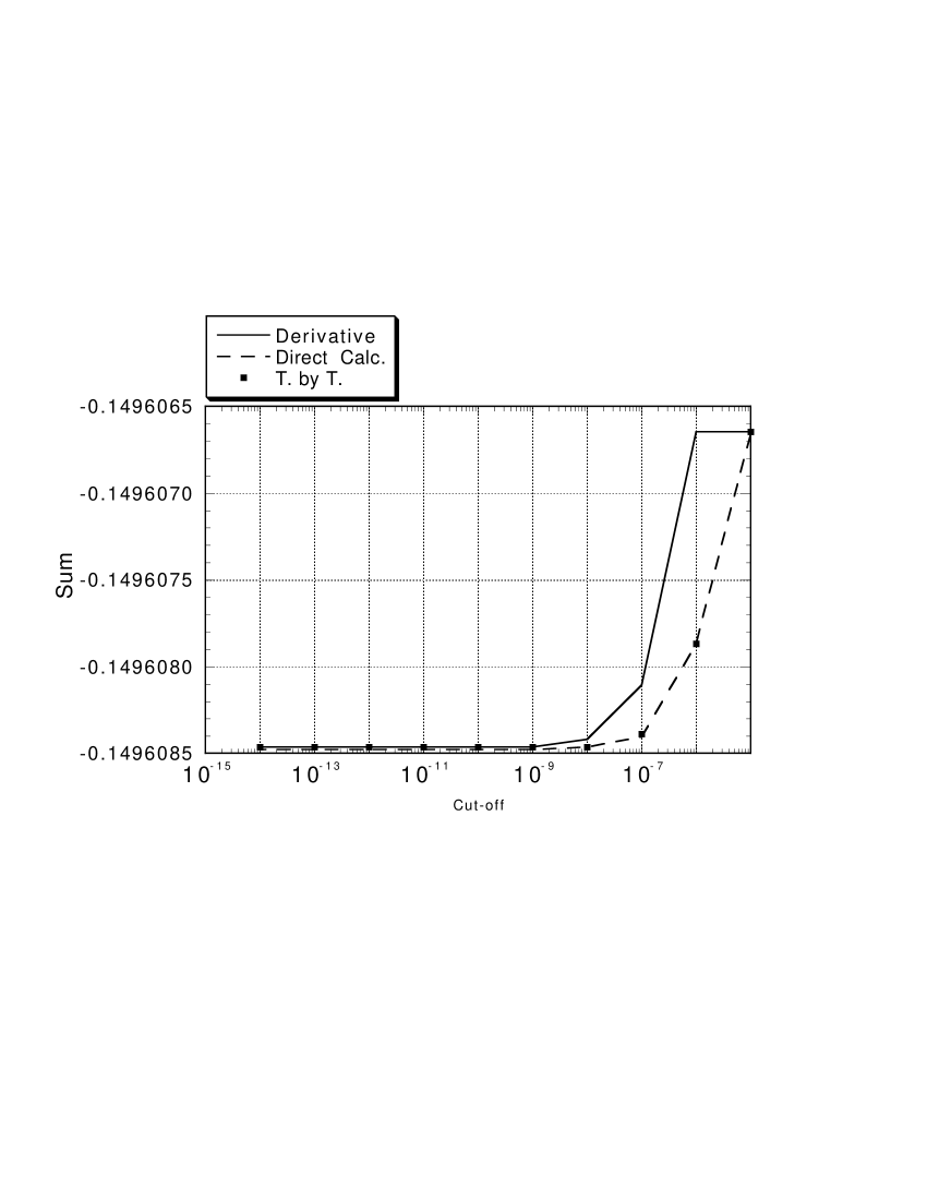
FIG. 4.: Comparison between the convergence of the sum calculated using numerical derivation of the unperturbed self-energy sum as in Eq. (150) to the direct evaluation using perturbed wave function and reduced Green’s function as defined in Eq. (199), and to an evaluation in which terms in Eqs. (151) to (159) are derived for each $\kappa$ value in the sum (T.-by-t deriv.). Evaluation is done for a $2p_{3/2}$ state and $r=0.9992$, $y=1$, $t=0.99$, $Z=20$.

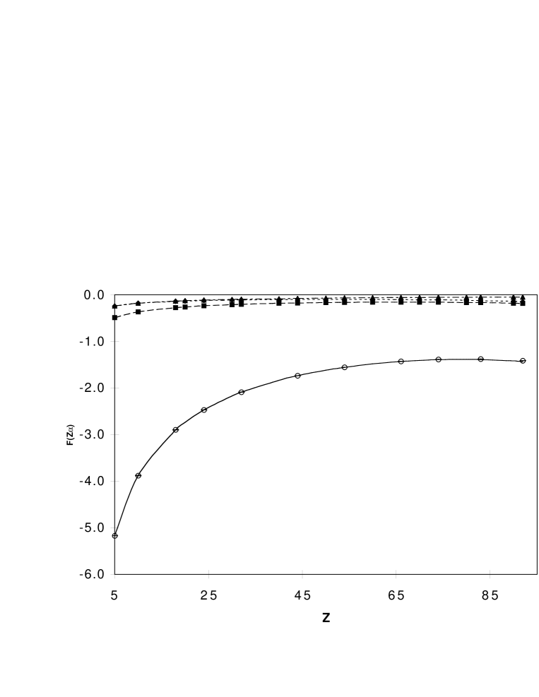
FIG. 5.: Screening of a $1s$ electron by a $1s$, $2s$, $2p_{1/2}$ or $2p_{3/2}$ electron. Sunnergren: Correction to the Coulomb part of the electron-electron interaction from Ref. [19], improved calculation following Ref. [3].

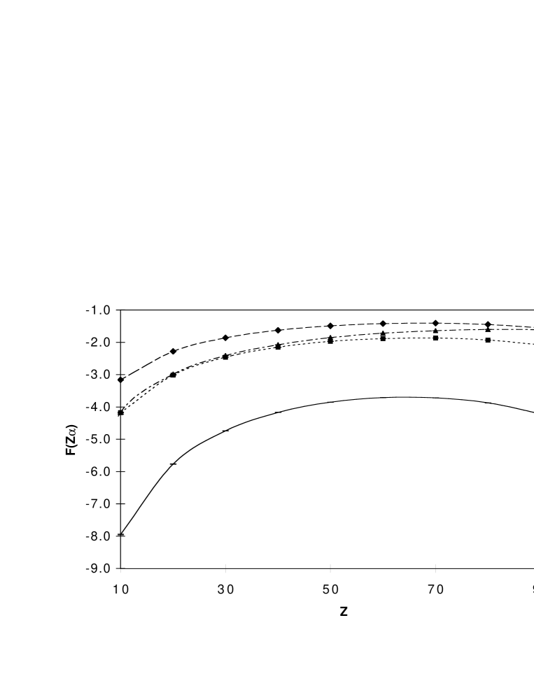
FIG. 6.: Screening of a $2s$ electron by a $1s$, $2s$, $2p_{1/2}$ or $2p_{3/2}$ electron.

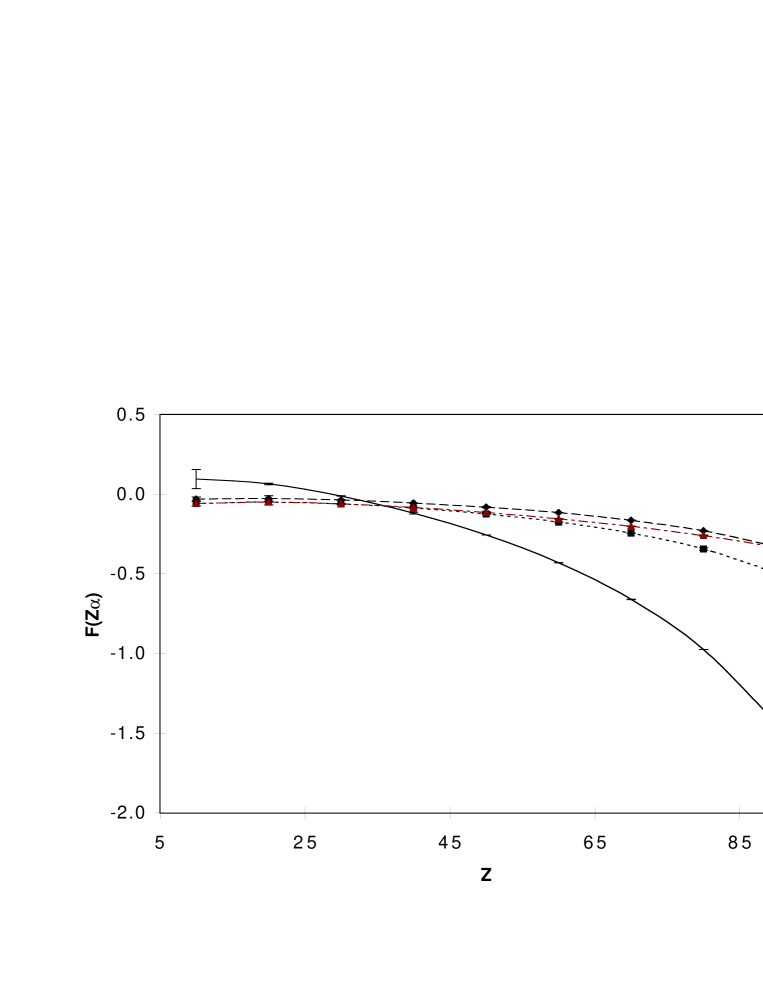
FIG. 7.: Screening of a $2p_{1/2}$ electron by a $1s$, $2s$, $2p_{1/2}$ or $2p_{3/2}$ electron.

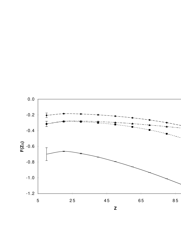
FIG. 8.: Screening of a $2p_{3/2}$ electron by a $1s$, $2s$, $2p_{1/2}$ or $2p_{3/2}$ electron. The large error bar for $Z=10$ are only due to the low-energy part of the vertex correction

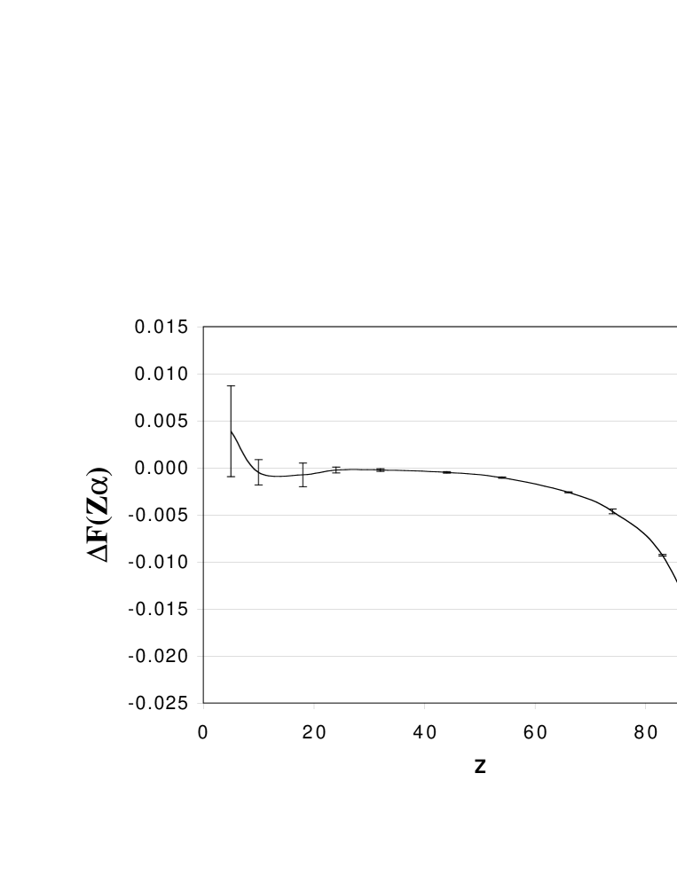
FIG. 9.: Comparison between calculation using the partial-wave renormalization method [3] and this work. More accurate numerical values from Ref. [19] are used.

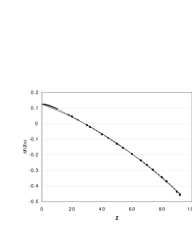
FIG. 10.: Comparison between calculation for point nucleus (including Coulomb and magnetic part of the electron-electron interaction) from Ref. [4] and the Coulomb value from this work. The solid line represents a second-order polynomial fit to the difference and extrapolates to $-0.124$ for $Z=0$, as expected from Eq. (225). Also plotted are the Breit values from Ref. [19], which are in reasonable agreement with the extrapolation.

REFERENCES

- [1] P. Indelicato and P. J. Mohr, Theor. Chem. Acta. 80, 207 (1991).
- [2] V. A. Yerokhin and V. M. Shabaev, Phys. Lett. A 207, 274 (1995).
- [3] H. Persson, S. Salomonson, P. Sunnergren, and I. Lindgren, Phys. Rev. Lett. 76, 204 (1996).
- [4] V. A. Yerokhin, A. N. Artemyev, and V. M. Shabaev, Phys. Lett. A 234, 361 (1997).
- [5] V. A. Yerokhin, A. N. Artemyev, T. Beier, V. M. Shabaev, and G. Soff, J. Phys. B: At. Mol Phys. 31, L691 (1998).
- [6] V. A. Yerokhin, A. N. Artemyev, T. Beier, V. M. Shabaev, and G. Soff, Phys. Scr. 59, in press (1998).
- [7] V. A. Yerokhin, A. N. Artemyev, T. Beier, G. Plunien, V. M. Shabaev, and G. Soff, Phys. Rev. A 60, 3522 (1999).
- [8] S. A. Blundell, K. T. Cheng, and J. Sapirstein, Phys. Rev. A 55, 1857 (1997).
- [9] P. J. Mohr, Ann. Phys. (N.Y.) 88, 26 (1974).
- [10] P. Indelicato and P. J. Mohr, Phys. Rev. A 46, 172 (1992).
- [11] P. Indelicato and P. J. Mohr, J. Math. Phys. 36, 714 (1995).
- [12] P. Indelicato and P. J. Mohr, Phys. Rev. A 58, 165 (1998).
- [13] D. J. Hylton, J. Math. Phys. 25, 1125 (1984).
- [14] P. J. Mohr and Y.-K. Kim, Phys. Rev. A 45, 2727 (1992).
- [15] P. J. Mohr, Ann. Phys. (N.Y.) 88, 52 (1974).
- [16] D. J. Hylton, Phys. Rev. A 32, 1303 (1985).
- [17] P. J. Mohr, G. Plunien, and G. Soff, Phy. Rep. 293, 227 (1998).
- [18] P. J. Mohr, Phys. Rev. A 26, 2338 (1982).
- [19] P. Sunnergren, Ph.D. thesis, Chalmers University of Technology, 1998.
- [20] U. D. Jentschura, P. J. Mohr, and G. Soff, Phys. Rev. Lett. 82, 53 (1999).
- [21] U. D. Jentschura, P. J. Mohr, G. Soff, and E. J. Weniger, Comp. Phys. Communi. 116, 28 (1999).
- [22] H. Araki, Prog. Theo. Phys 17, 619 (1957).
- [23] J. Sucher, Phys. Rev. 109, 1010 (1958).
- [24] G. W. F. Drake and W. C. Martin, Can. J. Phys. 76, 679 (1998).
- [25] G. W. F. Drake, in Atomic, Molecular and Optical Physics Handbook, edited by G. W. F. Drake (AIP Press, Woodbury, New York, 1996).
- [26] P. Indelicato, O. Gorceix, and J. P. Desclaux, J. Phys. B: At. Mol Phys. 20, 651 (1987).
- [27] P. Indelicato and J. P. Desclaux, Phys. Rev. A 42, 5139 (1990).
- [28] J. P. Desclaux, in Methods and Techniques in Computational Chemistry, edited by E. Clementi (STEF, Cagliary, 1993), Vol. A.
- [29] K. G. Dyall, I. P. Grant, C. T. Johnson, F. A. Parpia, and E. P. Plummer, Comp. Phys. Communi. 55, 425 (1989).
- [30] P. Indelicato, S. Boucard, and E. Lindroth, Eur. Phys. J. D 3, 29 (1998).
- [31] S. A. Blundell, Phys. Rev. A 46, 3762 (1992).
- [32] S. A. Blundell, Phys. Rev. A 47, 1790 (1993).
- [33] K. T. Cheng, W. R. Johnson, and J. Sapirstein, Phys. Rev. A 47, 1817 (1993).
- [34] H. Persson, I. Lindgren, S. Salomonson, and P. Sunnergren, Phys. Rev. A 48, 2772 (1993).
- [35] P. J. Mohr, Phys. Rev. A 46, 4421 (1992).