Dynamic fitness landscapes: Expansions for small mutation rates

Abstract

We study the evolution of asexual microorganisms with small mutation rate in fluctuating environments, and develop techniques that allow us to expand the formal solution of the evolution equations to first order in the mutation rate. Our method can be applied to both discrete time and continuous time systems. While the behavior of continuous time systems is dominated by the average fitness landscape for small mutation rates, in discrete time systems it is instead the geometric mean fitness that determines the system’s properties. In both cases, we find that in situations in which the arithmetic (resp. geometric) mean of the fitness landscape is degenerate, regions in which the fitness fluctuates around the mean value present a selective advantage over regions in which the fitness stays at the mean. This effect is caused by the vanishing genetic diffusion at low mutation rates. In the absence of strong diffusion, a population can stay close to a fluctuating peak when the peak’s height is below average, and take advantage of the peak when its height is above average.

1 Introduction

A major part of all living creatures on Earth consists of prokaryotes and phages. These organisms replicate mainly without sexual recombination [1], and typically produce offspring on a time-scale of hours. Because of their short gestation times, microbes experience ubiquitous environmental changes such as seasons on an evolutionary time scale. Most of the DNA based microbes have developed error correction mechanisms, such limiting the amount of deleterious mutations they experience. In a changing environment, however, small mutation rates might severely curtail a species’ ability to react to new situations. The observed genomic mutation rates of asexual organisms such as bacteria and DNA viruses lie typically around $2-4\times 10^{-3}$ [2], implying that a few out of every thousand offspring get mutated at all. It has been proposed [3] that even lower genomic mutation rates are not observed simply because they would stifle a species’ adaptability in a changing environment. While this is certainly a reasonable assumption, we do not currently have a deep understanding of what types of fitness landscapes require what mutation rates, and whether a small mutation rate is always disadvantageous in a changing environment. In this paper, we address the effects of a changing environment on a population evolving in a small mutation rate. Our main objective is to develop an expansion to first order in the mutation rate which enables us to find approximate solutions for infinite asexual populations evolving in arbitrary dynamic landscapes.

Due to the nature of the expansions that we use, we are led to a comparison between discrete time and continuous time systems. Our main result from the comparison is that in dynamic fitness landscapes, continuous and discrete time systems have qualitative differences in the low mutation rate regime. This difference can manifest itself, for example, in populations that replicate either continuously or synchronized in discrete generations. Given that all other factors are equal, the continuously replicating strains will have a selective advantage. As a generic result for both continuous and discrete time, we find that a low mutation rate can enable a population to draw a selective advantage from fluctuations in the landscape.

Our analysis is based on the quasispecies model [4, 5, 6]. The quasispecies literature was for a long time focused on static fitness landscapes, but recently more emphasis has been put on the aspect of changing environments [3, 7, 8, 9, 10, 11, 12, 13, 14]. Here, we mainly use methods developed in Ref. [12]. The paper is structured as follows. In Sec. 2, we demonstrate how systems with discrete as well as continuous time can be treated to first order in the mutation rate. In Sec. 3, we discuss the expansions we have found in Sec. 2. We treat the case of a vanishing mutation rate in Sec. 3.1, and that of a very small but positive mutation rate in Sec. 3.2. In Sec. 3.3, we study the localization of a population around a oscillating peak, and in Sec. 3.4, we discuss the problems we encounter when approximating a continuous time system with a discrete time system. We close our paper with concluding remarks in Sec. 4.

2 Analysis

2.1 The model

Consider a system of evolving bitstrings. The different bitstrings $i$ replicate with rates $A_{i}$, and they mutate into each other with probabilities $Q_{ij}$. Throughout this paper, we assume that the probability of an incorrectly copied bit is uniform over all strings, and denote this probability by $R$. The mutation matrix ${\mbox{Q}}=(Q_{ij})$ is then given by

$$Q_{ij}=(1-R)^{l}\left(\frac{R}{1-R}\right)^{d(i,j)}\,,$$ (1)

where $d(i,j)$ is the Hamming distance between two sequences $i$ and $j$. The matrix Q is a $2^{l}\times 2^{l}$ matrix, and it is in general difficult to handle numerically. Therefore, in the following we impose the additional assumption that all sequences with equal Hamming distance from a given reference sequence have the same fitness. This is the so-called error class assumption [15]. The matrix Q is then an $(l+1)\times(l+1)$ matrix,

$$Q_{ij}=\sum_{k=\max\{i+j-l,0\}}^{\min\{i,j\}}\binom{j}{k}\binom{l-j}{i-k}(1-R)^{l}\left(\frac{R}{1-R}\right)^{i+j-2k}\,.$$ (2)

The generality of our results is not affected by this choice, because the calculations we present in the following can be performed with either of the two matrices Q, and they lead to very similar expressions.

Let us write down the quasispecies equations for sequences evolving in continuous or discrete time and in a static fitness landscape. We introduce the replication matrix ${\mbox{A}}={\rm diag}(A_{0},A_{1},\dots)$. The continuous differential equation of the (unnormalized) concentration variables $\mbox{\boldmath$y$}=(y_{0},y_{1},\dots)$ then reads

$$\dot{\mbox{\boldmath$y$}}(t)={\mbox{Q}}{\mbox{A}}\mbox{\boldmath$y$}(t)\,.$$ (3)

The discrete difference equation, on the other hand, can be written as

$$\mbox{\boldmath$y$}(t+\Delta t)=[\Delta t{\mbox{Q}}{\mbox{A}}+\lambda]\mbox{\boldmath$y$}(t)\,,$$ (4)

where $\Delta t$ is the duration of one generation, and $\lambda$ gives the proportion of parents that survive one generation and enter the next one together with their offspring. Both Eq. (3) and Eq. (4) converge for $t\rightarrow\infty$ towards a sequence distribution given by the Perron eigenvector of the matrix QA. Hence, for a static landscape the discrete time and the continuous time quasispecies equations are equivalent, as far as the asymptotic state is concerned. The distinction between discrete and continuous time, however, is important when the fitness landscape changes over time. Consider the situation of a dynamic fitness landscape, represented by a time dependent matrix ${\mbox{A}}(t)$. Equation (3) becomes

$$\dot{\mbox{\boldmath$y$}}(t)={\mbox{Q}}{\mbox{A}}(t)\mbox{\boldmath$y$}(t)\,.$$ (5)

The time-dependent difference equation, on the other hand, reads

$$\mbox{\boldmath$y$}(t+\Delta t)=[\Delta t{\mbox{Q}}{\mbox{A}}(t)+\lambda]\mbox{\boldmath$y$}(t)\,,$$ (6)

The dynamic attractors of both Eqs. (5) and (6) are not immediately obvious, and therefore we cannot know to what extent the two systems differ unless we perform a more elaborate analysis. Moreover, in a static landscape, a nonzero $\lambda$ does not affect the asymptotic state of the system, which is why it normally is set to zero in Eq. (4) [16, 17]. The situation is different in a dynamic landscape, and we have to allow for a non-zero $\lambda$ in general.

2.2 Discrete time

Let us begin our analysis with the discrete system. We set $\lambda=0$, because that leads to the simplest equation describing a discrete time evolutionary system in a dynamic fitness landscape. The more complicated cases with $\lambda>0$ can be constructed from the equation for $\lambda=0$, as we will see later on. We address the equation

$$\mbox{\boldmath$y$}(t+\Delta t)=\Delta t{\mbox{Q}}{\mbox{A}}(t)\mbox{\boldmath$y$}(t)\,.$$ (7)

The solution to this equation is formally given by the time-ordered matrix product [12] [using $n=t/\Delta t$ and ${\mbox{A}}^{\prime}(\nu)=\Delta t\,{\mbox{A}}(\nu\Delta t)$]

$$\mbox{\boldmath$y$}(n) =\mathcal{T}\left\{\prod_{\nu=0}^{n-1}{\mbox{Q}}{\mbox{A}}^{\prime}(\nu)\right\}\mbox{\boldmath$y$}(0)$$

$$=:{\mbox{Y}}_{\rm disc}(n)\mbox{\boldmath$y$}(0)\,.$$ (8)

In the second line, we have introduced the notation ${\mbox{Y}}_{\rm disc}(n)$ for this matrix product. We will occasionally refer to ${\mbox{Y}}_{\rm disc}(n)$ as a propagator, since ${\mbox{Y}}_{\rm disc}(n)$ fully determines the state of the system at time $t=n\,\Delta t$, given an initial state at time $t=0$.

${\mbox{Y}}_{\rm disc}(n)$ can be evaluated to first order in $R$. The only dependency of ${\mbox{Y}}_{\rm disc}(n)$ on $R$ is the one in Q. When we expand Q [Eq. (2)] in $R$, we find

$$Q_{ij}=\sum_{k=\max\{i+j-l,0\}}^{\min\{i,j\}}\binom{j}{k}\binom{l-j}{i-k}[\delta_{\beta,0}+R(\delta_{\beta,1}-\alpha\delta_{\beta,0})+\dots]\,,$$ (9)

with $\alpha=l-\beta$ and $\beta=i+j-2k$. As usual, $\delta_{i,j}$ denotes the Kronecker symbol. The sum collapses into a single term, and we find to first order in $R$

$$Q_{ij}=(1-lR)\delta_{i,j}+(l-j)R\delta_{i,j+1}+jR\delta_{i,j-1}\,.$$ (10)

After some algebra, we obtain from that for the matrix ${\mbox{Y}}_{\rm disc}(n)$

$$\Big{(}{\mbox{Y}}_{\rm disc}(n)\Big{)}_{ij} =\left[(1-lRn)\prod_{\nu=0}^{n-1}A^{\prime}_{j}(\nu)\right]\delta_{i,j}$$

$$\qquad+\left[(l-j)R\sum_{\mu=0}^{t-1}\prod_{\nu_{1}=0}^{\mu}A^{\prime}_{j}(\nu_{1})\prod_{\nu_{2}=\mu+1}^{t-1}A^{\prime}_{j+1}(\nu_{2})\right]\delta_{i,j+1}$$

$$\qquad+\left[jR\sum_{\mu=0}^{t-1}\prod_{\nu_{1}=0}^{\mu}A^{\prime}_{j}(\nu_{1})\prod_{\nu_{2}=\mu+1}^{t-1}A^{\prime}_{j-1}(\nu_{2})\right]\delta_{i,j-1}\,,$$ (11)

This expression fully describes to first order in $R$ the state of the system after $n$ time steps.

2.3 Continuous time

Let us now turn to the continuous system. We can use the expansion of ${\mbox{Y}}_{\rm disc}(n)$ to find an expansion for the propagator of the static continuous case. If the fitness landscape is static, the solution to Eq. (3) is given by

$$\mbox{\boldmath$y$}(t)=\exp({\mbox{Q}}{\mbox{A}}t)\mbox{\boldmath$y$}(0)\,.$$ (12)

It is useful to recall that the exponential operator of a matrix is defined as

$$\exp({\mbox{Q}}{\mbox{A}}t)=\mbox{\boldmath$1$}+{\mbox{Q}}{\mbox{A}}t+\frac{1}{2!}({\mbox{Q}}{\mbox{A}}t)^{2}+\dots\,.$$ (13)

We can expand the single terms in that sum separately. Equation (2.2) allows us to write $({\mbox{Q}}{\mbox{A}})^{k}$ as

$$\Big{(}({\mbox{Q}}{\mbox{A}})^{k}\Big{)}_{ij} =(1-klR)A_{j}^{k}\delta_{i,j}+\left[(l-j)R\sum_{\mu=1}^{k}A_{j}^{\mu}A_{j+1}^{k-\mu}\right]\delta_{i,j+1}$$

$$\qquad+\left[jR\sum_{\mu=1}^{k}A_{j}^{\mu}A_{j-1}^{k-\mu}\right]\delta_{i,j-1}+\mathcal{O}(R^{2})\,.$$ (14)

Both the sums in the expression for $({\mbox{Q}}{\mbox{A}})^{k}$ and the remaining sum in Eq. (13) can then be taken analytically. We find

$$\Big{(}\exp({\mbox{Q}}{\mbox{A}}t)\Big{)}_{ij} =(1-lRA_{j}t)e^{A_{j}t}\delta_{i,j}+(l-j)RK[A_{j}t,A_{j+1}t]\delta_{i,j+1}$$

$$\qquad+jRK[A_{j}t,A_{j-1}t]\delta_{i,j-1}\,,$$ (15)

where the function $K[a,b]$ is of the form

$$K[a,b]=\frac{a}{a-b}\left(e^{a}-e^{b}\right).$$ (16)

With Eq. (2.3), we have an expansion of the propagator of the continuous system in a static landscape to first order in $R$. Similarly, we can treat piecewise constant landscapes. Under a piecewise constant landscape we understand a landscape for which we can define intervals $I_{1}=[0,t_{1})$, $I_{2}=[t_{1},t_{2})$, $I_{3}=[t_{2},t_{3})$, $\dots$, such that the landscape does not change within any of these intervals. Any dynamic fitness landscape can be approximated in that way. The solution to the differential equation for that type of landscapes is given by

$$\mbox{\boldmath$y$}(t) =\exp[{\mbox{Q}}{\mbox{A}}(t_{n})(t-t_{n})]\exp[{\mbox{Q}}{\mbox{A}}(t_{n-1})(t_{n}-t_{n-1})]\cdots$$

$$\qquad\cdots\exp[{\mbox{Q}}{\mbox{A}}(0)t_{1}]\mbox{\boldmath$y$}(0)\,.$$ (17)

With the two simplifying assumptions that all intervals have the same length $\tau$ and that we are observing the system only at the end of an interval, Eq. (2.3) becomes (for $n=t/\tau$)

$$\mbox{\boldmath$y$}(t) =\mathcal{T}\left\{\prod_{\nu=0}^{n-1}\exp[{\mbox{Q}}{\mbox{A}}(\nu\tau)\tau]\right\}\mbox{\boldmath$y$}(0)$$

$$=:{\mbox{Y}}_{\rm cont}(t)\mbox{\boldmath$y$}(0)\,.$$ (18)

The similarity to Eq. (2.2) is evident. Hence, in analogy to the calculation that leads from Eq. (10) to Eq. (2.2), we find in the piecewise constant, continuous case

$$\Big{(}{\mbox{Y}}_{\rm cont}(t)\Big{)}_{ij}=\left[\Big{(}1-lR\sum_{\nu=0}^{n-1}A_{j}^{c}(\nu)\Big{)}\exp\Big{(}\sum_{\nu=0}^{n-1}A_{j}^{c}(\nu)\Big{)}\right]\delta_{i,j}\\ \qquad+\left[(l-j)R\sum_{\mu=0}^{n-1}K^{(\mu)}_{j,j+1}\prod_{\nu_{1}=0}^{\mu-1}\exp[A_{j}^{c}(\nu_{1})]\prod_{\nu_{2}=\mu+1}^{n-1}\exp[A_{j+1}^{c}(\nu_{2})]\right]\delta_{i,j+1}\\ \qquad+\left[jR\sum_{\mu=0}^{n-1}K^{(\mu)}_{j,j-1}\prod_{\nu_{1}=0}^{\mu-1}\exp[A_{j}^{c}(\nu_{1})]\prod_{\nu_{2}=\mu+1}^{n-1}\exp[A_{j-1}^{c}(\nu_{2})]\right]\delta_{i,j-1}\,.$$ (19)

We have used the abbreviations

$${\mbox{A}}^{c}(\nu)=\tau{\mbox{A}}(\nu\tau)\quad\mbox{and}\quad K^{(\nu)}_{i,j}=K[A_{i}^{c}(\nu),A_{j}^{c}(\nu)].$$ (20)

Equation (19) fully determines to first order in $R$ the state of the continuous system after $t$ units of time have passed.

3 Discussion

With Eqs. (2.2) and (19), we have expansions for the propagators of discrete-time and continuous time evolving systems in a dynamic fitness landscape. In this section, we will examine these expansions and discuss their properties.

3.1 A vanishing mutation rate

For $R=0$, both ${\mbox{Y}}_{\rm disc}(t)$ and ${\mbox{Y}}_{\rm cont}(t)$ turn into diagonal matrices. We find (choosing $\tau=\Delta t$ and $n=t/\tau$)

$$Y_{\rm disc}(t) =\exp\big{[}\sum_{\nu=0}^{n-1}\log\big{(}{\mbox{A}}^{\prime}(\nu)\big{)}\big{]}=\left(\!\sqrt[\scriptstyle n]{{\mbox{A}}^{\prime}(n-1)\cdots{\mbox{A}}^{\prime}(0)}\,\right)^{n}\,,$$ (21)

$$Y_{\rm cont}(t) =\exp\big{[}\sum_{\nu=0}^{n-1}{\mbox{A}}^{c}(\nu)\big{]}\,.$$ (22)

This result shows that in a dynamic fitness landscape the discrete and the continuous model have not only quantitative, but also important qualitative differences. While in the continuous case the state of the system at time $t$ is determined by the exponential of the arithmetic mean of the fitness landscape until time $t$, in the discrete case it is determined by the exponential of the geometric mean of the fitness landscape, which can be written as arithmetic mean of the logarithm of the fitness landscape. The latter corresponds to results from population genetics [18]. Since arithmetic and geometric mean are in general different, the same fitness landscape can have very different effects in a continuous or discrete system for $R=0$. Consider a landscape, for example, with an oscillating sharp peak,

$$A_{0}(t) =\begin{cases}\sigma(1-a)\qquad\mbox{for $\phantom{T/}0\leq t<T/2$}\\ \sigma(1+a)\qquad\mbox{for $T/2\leq t<T$}\end{cases}$$ (23a)

$$A_{i}(t) =1\qquad\mbox{for $0<i\leq l$}\,,$$ (23b)

with $0\leq a<1$ and $\sigma>0$.

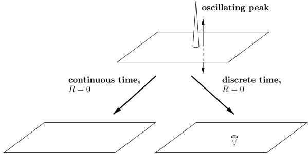
Figure 1: A landscape with an oscillating peak whose average height coincides with the fitness of all other sequences. In continuous time, the landscape becomes completely flat for $R=0$. In discrete time, however, the population feels the geometric mean of the fitness landscape for $R=0$, which has a hole at the position of the peak.

In the continuous system without mutations, the master sequence grows with the rate $\overline{A}_{0}=\sigma$ if time is measured in integer multiples of $T$. Hence, if $\sigma>1$, the peak sequence will always supersede all other sequences for $t\to\infty$. Contrasting to that, the geometric mean is $\widetilde{A}_{0}=\sigma\sqrt{1-a^{2}}$. Even for $\sigma>1$ it is possible to have $\widetilde{A}_{0}<1$ if $a$ is large enough, in which case in the discrete system the master sequence grows slower than all others. Consequently, it will be expelled from the population for $t\to\infty$. The special case of $\sigma=1$ is depicted in Fig. 1. There, the fitness landscape becomes flat in continuous time, but acquires a hole in discrete time.

3.2 Small non-zero mutation rates

Let us now turn to the case of a small but non-zero $R$. From the above, we can expect that there is a qualitative difference between discrete and continuous time even for finite $R$. In order to see this difference, we take the oscillating sharp peak landscape as a generic example. A two concentration approximation has proven useful to describe situations with $\sigma\gg 1$ [14] but is not applicable here, since we are particularly interested in the case $\sigma=1$, for which the average landscape is flat in continuous time and acquires a hole in discrete time.

The analysis of the landscape Eq. (23) is facilitated by its periodicity in time (with period length $T$). For periodic landscapes, it has been shown in Ref. [12] that a periodic attractor with period length $T$ exists. Its state at phase $\phi=0$ (the phase is defined as $\phi:=t\;\mbox{mod}\;T$) is given by the principal eigenvector of the monodromy matrix

$${\mbox{X}}(0)={\mbox{Y}}(T)\,,$$ (24)

where ${\mbox{Y}}(t)$ is the propagator of the system. Equation (24) holds regardless of continuous or discrete time. The attractor’s state at other phases $\phi$ can be calculated in a similar fashion.

In Figure 2, we have displayed the order parameter $m_{s}$ [19, 20] in the sharp peak landscape as a function of $R$ for the discrete time and the continuous time system. The order parameter is given by

$$m_{s}(t)=\frac{1}{l}\sum_{i=0}^{l}x_{i}(t)(l-2i)\,,$$ (25)

where the $x_{i}(t)$ represent the total (normalized) concentration of all sequences in error class $i$ at time $t$. We have calculated the order parameter both from the full monodromy matrix and from the expansions to first order in $R$. We find that the expansions give reliable results for small mutation rates, but start deviating from the true value as $R$ approaches $1/lT$. Note that both expansions must break down beyond $1/lT$, as both the discrete and the continuous propagator assume unphysical negative values on the diagonal when $R$ exceeds $1/lT$ [Eqs. (2.2) and (19)].

From Fig. 2, it is evident that there exists a qualitative difference between the discrete and the continuous time system. In the system with continuous time, the sequences stay centered around the currently active peak for arbitrarily small but non-zero mutation rates, whereas in the system with discrete time, the sequence distribution becomes ever more homogeneous as $R\rightarrow 0$.

The behavior of the discrete system is easily explained. In the geometric mean of the landscape, the peak position is actually disadvantageous, and hence the population is driven into the remaining genotype space, which it occupies homogeneously due to the lack of selective differences. Formally, the population feels the geometric mean only for a vanishing mutation rate. However, by continuity, the disadvantage at the peak position will remain for some small but non-zero $R$, which leads to the continuous decay of the order parameter as $R\rightarrow 0$. Interestingly, the order parameter does not decay exactly to zero, but to a value slightly below zero. This happens because the population becomes homogeneously distributed over the whole sequence space except for the position of the oscillating peak. The resulting small imbalance in the sequence distribution towards the opposite end of the boolean hypercube then leads to a negative order parameter. The inset in Fig. 2 shows that our approximation predicts this behavior accurately for small $R$.

Now consider the continuous system. For an infinitesimal $R>0$, the dependence of the asymptotic state on the initial condition is lost, as we know from the Frobenius-Perron theorem. Since for $R=0$ the evolution of the population in time steps of size $T$ is guided by the flat average landscape, one might suspect that for infinitesimal $R>0$ a homogeneous distribution is found as the unique asymptotic state. This is what we observe for a population evolving in a flat static landscape with little mutation. However, the situation in a dynamic landscape may be different, because the dynamics of the landscape has a significant influence on the asymptotic sequence distribution. In fact, it is possible that a flat average landscape leads to an ordered asymptotic state for finite mutation rates $R>0$. In the next subsection, we will demonstrate this effect for the oscillating sharp peak.

3.3 Localization around an oscillating peak

We will now have a closer look at the oscillating sharp peak landscape, Eq. (23). We are interested in the case $\sigma=1$, which leads to a degenerate average in continuous time. First we note some general properties of the monodromy matrix ${\mbox{X}}(\phi)$ for a periodic landscape with flat arithmetic mean. If ${\mbox{X}}(\phi)$ is given to first order in $R$, it reads (assuming the average fitness is 1)

$${\mbox{X}}(\phi)=(1-TlR){\mbox{1}}+R\tilde{{\mbox{X}}}(\phi)\,,$$ (26)

where $\tilde{{\mbox{X}}}(\phi)$ is independent of the mutation rate $R$ and contains only the off-diagonal entries from Eq. (19). Since $\tilde{{\mbox{X}}}(\phi)$ differs from ${\mbox{X}}(\phi)$ only by a scalar factor and an additional constant on the diagonal, the eigenvectors of the former matrix are identical to the ones of the latter matrix, while the eigenvalues are related through $\lambda_{i}=(1-TlR)+R\tilde{\lambda}_{i}$. As a consequence, we find that the asymptotic species distribution is given by the principal eigenvector of the off-diagonal matrix $\tilde{{\mbox{X}}}(\phi)$, which is independent of $R$. If we took terms up to the $k$th order of $R$ into account in Eq. (19), we would find the higher order contributions to the eigenvectors up to $(k-1)$th order of $R$. However, with our first-order approximation, we are only able to calculate the asymptotic sequence concentrations to 0th order in $R$.

For small mutation rates $R$, we can restrict our analysis to the first three error classes. For the oscillating peak, we find with help of Eq. (19) the following expressions

$$\tilde{{\mbox{X}}}(\phi)\approx T\exp(T)\left(\begin{matrix}0&\alpha_{\phi}(aT)&0\\ l\beta_{\phi}(aT)\alpha_{\phi}(aT)&0&2\\ 0&l-1&0\end{matrix}\right)\,,$$ (27)

where

$$\alpha_{\phi}(\xi) =(2/\xi)[1-e^{-\xi/2}]e^{\xi|\phi-1/2|}\,$$ (28a)

$$\beta_{\phi}(\xi) =e^{\xi/2}e^{-2\xi|\phi-1/2|}\,$$ (28b)

$$\xi =aT\,.$$ (28c)

The (unnormalized) asymptotic state follows as

$$\left(\begin{matrix}y_{0}\\ y_{1}\\ y_{2}\end{matrix}\right)(\phi,\xi)=\left(\begin{matrix}\alpha_{\phi}(\xi)\\ \sqrt{2(l-1)+\alpha_{\phi}^{2}(\xi)\beta_{\phi}(\xi)\,l}\\ l-1\end{matrix}\right)\,.$$ (29)

Now, if the third error class concentration is negligibly small compared to the other two concentrations, the concentrations of the higher error classes can be neglected as well, and the asymptotic state is approximately given by the concentrations of the first two error classes only. From Eq. (29), we can derive the following criterion for this approximation to be valid,

$$\exp(\xi/2)\gg l\xi^{2}/4.$$ (30)

Hence, if $\xi=aT$ is large, which means that the fitness fluctuations are large and slow, the population is exclusively distributed over the peak and the first error class. For this case, we find the following simplified description of the population:

$$x_{0}(\phi,\xi) =1\Big{/}\left[1+\sqrt{l\beta_{\phi}(\xi)}\right]\,,$$ (31a)

$$x_{1}(\phi,\xi) =\sqrt{l\beta_{\phi}(\xi)}\Big{/}\left[1+\sqrt{l\beta_{\phi}(\xi)}\right]\,,$$ (31b)

$$m_{s}(\phi,\xi) =1-2x_{1}(\phi,\xi)/l\,.$$ (31c)

The last equation implies that in the limit $R\to 0$, the order parameter is always larger than $1-2/l$. This means that although the peak does not have an average selective advantage, the evolving sequences are attracted to the peak nonetheless. As long as $l>1$, the order parameter averaged over one oscillation cycle is positive, which means that a population can draw a selective advantage from being close to the peak in comparison to being far away from it.

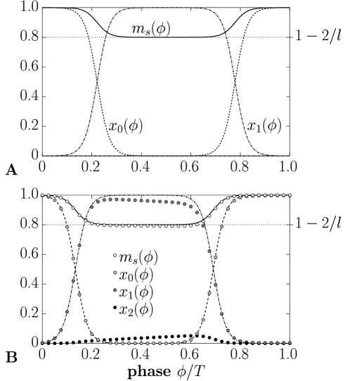
Figure 3: Sequence concentrations and order parameter of the steady state versus the relative phase $\phi/T$. The upper plot (A) shows the predictions for $R\to 0$ from the three-concentration model [Eq. (31)], with $T=100$, $a=0.4$ and $l=10$. The line for $x_{2}(\phi)$ is indistinguishable from the abscissa. For sufficiently small mutation rates and given Eq. (30), the full numeric solution is in perfect agreement with the three-concentration model. For larger mutation rates, the main discrepancy arises as a phase shift. For $R=10^{-4}$ (B), the prediction is still in good agreement with the full numeric solution (shown as circles) if we phase-shift our prediction by an amount of $\Delta\phi/T=0.088$.

In Figure 3A, we display the predicted behavior of the system in a very small mutation rate, as given by Eq. (31). The observed change in the sequence concentrations is explained as follows. During the times at which the peak has above-average fitness, the sequences on the peak replicate faster than all others and hence grow exponentially until the peak’s concentration saturates around one, while all off-peak sequences assume vanishing concentrations. Similarly, during the times at which the peak has below-average fitness, the peak’s relative concentration decays, while the population moves onto the nearest advantageous sequences, which can be found in the first error class. The sequences in all other error classes are adaptively neutral compared to the first error class. Hence, the amount of sequences that move into higher error classes is solely determined by the mutation rate. If the mutation rate is small enough, the diffusion among these neutral sequences becomes negligibly small on the time scale of the peak oscillations $T$. Therefore, the population stays mainly within the first error class until the peak fitness switches back to the above-average value. Thus, we find the qualitative behavior of Eq. (31): In a landscape with a large and slowly oscillating sharp peak and a small mutation rate, the population oscillates between the peak sequence and the first error class in the asymptotic state. In short, the population becomes localized close to the peak.

For extremely small mutation rates, Eq. (31) agrees perfectly with the full numerical solution. For somewhat larger mutation rates, the main discrepancy that arises is a phase shift between the full solution and the approximation (Figure 3B). The phase shift moves the concentration curves towards earlier times, i.e., the system becomes more responsive to the changing peak as the mutation rate increases. This is intuitively clear. With a higher mutation rate, the first error class will already be occupied to a larger extent when the peak switches to the below-average value, so that the concentration of the one-mutants can grow faster towards their equilibrium value. Similarly, when the peak switches back to the above-average value, the peak sequences have a more favorable initial concentration, which makes them grow faster in comparison to a lower mutation rate.

Let us shortly extend the above argumentation to broader peaks, like peaks with linear flanks of width $1\leq w\leq l$:

$$A_{i}(t)=\max\Big{\{}1,\,\frac{w-i}{w}[A_{0}(t)-1]\Big{\}}\quad\mbox{for all $0<i\leq l$}.$$ (32)

The sharp peak from above corresponds to a peak of width $w=1$. For arbitrary chosen width $1\leq w\leq l$, the population gets transported to the $w$th error class due to the selection pressure during the below-average peak fitness phases. The $w$th error class is in that case the boundary of the advantageous region. Again, if the mutation rate is sufficiently small, diffusion can be neglected and the population will stay in the $w$th error class until the peak fitness switches back to the above-average value. This implies that for peaks of width $w\geq l/2$, it is possible to have $m_{s}(\phi)\leq 0$ for some intermediate oscillation phases. In particular for the maximum width $w=l$, the order parameter $m_{s}(\phi)$ will oscillate symmetrically around zero.

In this subsection, we have only considered continuous time systems. We have established that in a dynamic fitness landscape with flat average, a population can draw a selective advantage from peaks that fluctuate around the average fitness value. The same effect will occur in a discrete time system if we consider the geometric mean of the fitness landscape instead. In other words, in a landscape with flat geometric mean, a population with a small mutation rate will draw a selective advantage from a peak that fluctuates around that geometric mean. The origin of that effect is again the vanishing diffusion, which causes the population to remain close to the peak when the peak has a height below the mean.

3.4 Discrete systems with overlapping generations

When discussing the discrete system in Sec. 3.1 and 3.2, we have set $\lambda=0$, i.e., we have made the assumption that every sequence can generate offspring only once, and dies before the next generation starts to replicate. The opposite extreme is $\lambda=1$, for which no sequence ever dies. With $\lambda=1$, a sequence can theoretically stay infinitely long in the system (in practice, the growth of new sequences is compensated through an out-flux of old sequences, but that is not our concern here. The details of the out-flux do not influence the unnormalized concentration variables $\mbox{\boldmath$y$}(t)$ in Eqs. (3)–(6) [12]). For $\lambda=1$, Eq. (6) converges to Eq. (5) for $\Delta t\rightarrow 0$. In other words, for $\lambda=1$ and a small $\Delta t$, Eq. (6) is an approximation to Eq. (5). This fact has been exploited in Ref. [12] in order to calculate the continuous system numerically. However, it has not been evaluated in Ref. [12] to what extend the discrete approximation behaves qualitatively different from the continuous system.

Let us briefly examine how the discrete equation with $\lambda=1$ fits into the concepts we have developed so far. For $\lambda=1$, the propagator ${\mbox{Y}}_{\rm disc}(t)$ assumes the form

$${\mbox{Y}}_{\rm disc}(t)=\mathcal{T}\left\{\prod_{\nu=0}^{n-1}[\Delta t{\mbox{Q}}{\mbox{A}}(\nu\Delta t)+1]\right\}\,,$$ (33)

which can be rewritten into

$${\mbox{Y}}_{\rm disc}(t) =\mathcal{T}\bigg{\{}\mbox{\boldmath$1$}+\Delta t\sum_{\nu=0}^{n-1}{\mbox{Q}}{\mbox{A}}(\nu\Delta t)+\Delta t^{2}\sum_{\nu=0}^{n-1}\sum_{\nu^{\prime}=0}^{\nu-1}{\mbox{Q}}{\mbox{A}}(\nu\Delta t){\mbox{Q}}{\mbox{A}}(\nu^{\prime}\Delta t)$$

$$\qquad\qquad+\dots+\Delta t^{n}\prod_{\nu=0}^{n-1}{\mbox{Q}}{\mbox{A}}(\nu\Delta t)\bigg{\}}\,.$$ (34)

With the formulae given in Section 2, it is possible to expand this expression to first order in $R$. Since the corresponding calculation is tedious, and the result does not give any new insights, we omit this expansion here. Let us just consider the zeroth order term,

$${\mbox{Y}}_{\rm disc}(t) =\mbox{\boldmath$1$}+\Delta t\sum_{\nu=0}^{n-1}{\mbox{A}}(\nu\Delta t)+\Delta t^{2}\sum_{\nu=0}^{n-1}\sum_{\nu^{\prime}=0}^{\nu-1}{\mbox{A}}(\nu\Delta t){\mbox{A}}(\nu^{\prime}\Delta t)$$

$$\qquad\qquad+\dots+\Delta t^{n}\prod_{\nu=0}^{n-1}{\mbox{A}}(\nu\Delta t)+\mathcal{O}(R)\,.$$ (35)

Compare this expression to Eqs. (21) and (22). For $\lambda=1$, we neither have the exponential of the averaged landscape, nor do we have an expression that depends solely on the geometric mean of the landscape. We obtain a mixture between the two cases, and the size of $\Delta t$ determines which case we are closer to. Consequently, we obtain qualitatively wrong results from the discrete approximation if the arithmetic and geometric mean of the landscape differ significantly. Nevertheless, the discrepancies between the results can be restricted to arbitrary small values of the mutation rate if we choose $\Delta t$ small enough.

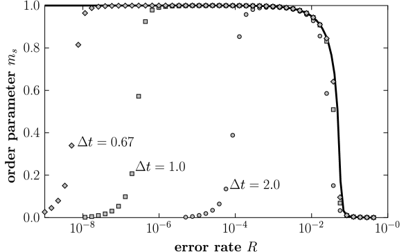
Figure 4: Order parameter in a fitness landscape similar to that of Fig. 2, but with $T=100$. The solid line stems from the full continuous time propagator, and the dots have been calculated from the discrete approximation Eq. (33). The number of discretization time steps $n$ is defined as $T/\Delta t$. The graph shows a snapshot of the order parameter at phase $\phi=0$ of its limit cycle.

As an example, consider Fig. 4. There we display the order parameter in the oscillating sharp peak landscape obtained from the full continuous propagator, and compare it to the result from the discrete approximation for various values of $\Delta t$. For a relatively large $\Delta t=2$ ($n=50$), Eq. (33) gives a poor approximation of the continuous system. Throughout the whole range of $R$ there are significant deviations from the full solution. As we decrease $\Delta t$ (increase $n$), the approximation moves much closer to the true value of the order parameter. Yet, for very small $R$, the order parameter always decays to zero in the approximation, whereas it stays close to one in the full solution. However small we choose $\Delta t$, there will always be some contribution from the geometric mean at $R=0$. That causes the order parameter in the discrete approximation to vanish for this particular landscape.

Contrasting to above situation, however, the differences between approximation and full solution are hardly noticeable in landscapes where the arithmetic and the geometric mean have a comparable structure (a peak in the averaged landscape is also a peak in the geometric mean of the geometric mean of the landscape, only with a slightly different height).

4 Conclusions

We have studied time-dependent fitness landscapes in the quasispecies model for the particular regime of small mutation rates. We have shown that the discrete time formulation and the continuous time formulation yield qualitatively different outcomes in that regime. If time is updated continuously, an evolving population adapts for $R\rightarrow 0$ to the exponential of the average fitness landscape, whereas in discrete time, the population adapts to the geometric mean of the landscape.

If the arithmetic or the geometric mean of the fitness landscape have degeneracies, then the behavior of the respective continuous time or discrete time system for $R\rightarrow 0$ is determined by the effect of the landscape on the population for some small but finite $R$, which can be very different from its effect for $R=0$. In particular, for the case of a slowly oscillating peak, the growth of the population onto the peak when the peak is high is much faster than the diffusion away from the peak when the peak is low, which implies that a population can draw a selective advantage from that peak even if the average (resp. geometric mean) height of the peak does not exceed the surrounding landscape. From that observation, the following picture emerges: If the average height of a slowly oscillating peak is larger than or equal to the surrounding fitness landscape, than in a small mutation rate environment a population will draw a selective advantage from being close to the peak position. Only if the average height is truly smaller than the surrounding fitness, the peak position will be necessarily disadvantageous.

The differences that we have found between continuous time and discrete time systems are not only interesting from a modeling perspective. They also have implications for the evolution of organisms that have the ability to influence their replication cycle. In a fluctuating environment, a strain that feels the average of the landscape will have a selective advantage over a strain that feels the geometric mean, as the latter is generally smaller. Hence, if two strains are identical apart from the fact that one replicates in a synchronized manner (all individuals generate their offspring at the same time, every $\Delta t$ units of time), whereas the other one replicates unsynchronized (at any point in time, some individuals may generate offspring), then the unsynchronized strain will out-compete the synchronized strain.

Throughout this paper, we have exclusively considered infinite populations. It is quite likely that finite populations experience the arithmetic or geometric mean fitness just as infinite populations do. However, since finite population sampling occurs at every time step, the sampling might well interfere with the averaging, such that finite populations could experience a somewhat different landscape. Nevertheless, the effect that a fluctuating peak can lead to a selective advantage will also exist in a finite population. With a small mutation rate, the finite population will not drift away from the peak when it is below average, and hence the population will most likely rediscover the peak when it rises again to above average.

We thank Erik van Nimwegen for useful comments and suggestions, and Chris Adami for carefully reading the manuscript. This work was supported in part by the National Science Foundation under contract No. DEB-9981397, and by the BMBF under Förderkennzeichen 01IB802C4.

Figure 2: Order parameter $m_{s}$ in a dynamic fitness landscape with a single oscillating peak in a continuous time system and a discrete time system. The solid lines have been obtained from diagonalizing the full monodromy matrix X, the dotted lines represent the approximation to first order in $R$. We have used the fitness landscape defined in Eq. (23), with $a=8/10$, $T=30$, and $l=10$. The graph shows a snapshot of the order parameter at phase $\phi=0$ of its limit cycle. The inset shows the same data, but in a log-log plot. There, we have plotted the absolute value of $m_{s}$ for the discrete-time system, because $m_{s}$ assumes a value slightly below 0 in that case.

References

- [1] Bruce R. Levin and Carl T. Bergstrom. Bacteria are different: Observations, interpretations, speculations, and opinions about the mechanisms of adaptive evolution in prokaryotes. Proc. Natl. Acad. Sci. USA, 97:6981–6985, 2000.
- [2] J. W. Drake, B. Charlesworth, D. Charlesworth, and J. F. Crow. Rates of spontaneous mutations. Genetics, 148:1667–1686, 1998.
- [3] Martin Nilsson and Nigel Snoad. Optimal mutation rates in dynamic environments. eprint physics/0004042, April 2000.
- [4] M. Eigen. Selforganization of matter and the evolution of biological macromolecules. Naturwissenschaften, 58:465–523, 1971.
- [5] Manfred Eigen, John McCaskill, and Peter Schuster. Molecular quasi-species. J. Phys. Chem., 92:6881–6891, 1988.
- [6] Manfred Eigen, John McCaskill, and Peter Schuster. The molecular quasi-species. Adv. Chem. Phys., 75:149–263, 1989.
- [7] B. L. Jones. Selection in systems of self-reproducing macromolecules under the constraint of controlled energy fluxes. Bull. Math. Biol., 41:761–766, 1979.
- [8] B. L. Jones. Some models for selection of biological macromolecules with time varying constants. Bull. Math. Biol., 41:849–859, 1979.
- [9] Claus O. Wilke. Evolutionary Dynamics in Time-Dependent Environments. Shaker Verlag, Aachen, 1999. PhD thesis Ruhr-Universität Bochum.
- [10] Claus O. Wilke, Christopher Ronnewinkel, and Thomas Martinetz. Molecular evolution in time dependent environments. In Dario Floreano, Jean-Daniel Nicoud, and Francesco Mondada, editors, Advances in Artificial Life, Proceedings of ECAL’99, Lausanne, Switzerland, Lecture Notes in Artificial Intelligence, pages 417–421, New York, 1999. Springer-Verlag.
- [11] Martin Nilsson and Nigel Snoad. Error thresholds on dynamic fitness landscapes. Phys. Rev. Lett., 84:191–194, 2000.
- [12] Claus O. Wilke, Christopher Ronnewinkel, and Thomas Martinetz. Dynamic fitness landscapes in molecular evolution. Phys. Rep., in press. (eprint physics/9912012).
- [13] C. Ronnewinkel, C. O. Wilke, and T. Martinetz. Genetic algorithms in time-dependent environments. In L. Kallel, B. Naudts, and A. Rogers, editors, Theoretical Aspects of Evolutionary Computing, New York, 2000. Springer-Verlag.
- [14] Martin Nilsson and Nigel Snoad. Quasispecies evolution on a fitness landscape with a fluctuating peak. eprint physics/0004039, April 2000.
- [15] Jörg Swetina and Peter Schuster. Self-replication with errors—A model for polynucleotide replication. Biophys. Chem., 16:329–345, 1982.
- [16] Lloyd Demetrius, Peter Schuster, and Karl Sigmund. Polynucleotide evolution and branching processes. Bull. Math. Biol., 47:239–262, 1985.
- [17] Ellen Baake and Wilfried Gabriel. Biological evolution through mutation, selection and drift: An introductory review. Ann. Rev. Comp. Phys., 7, 1999. in press.
- [18] Jin Yoshimura and Vincent A. A. Jansen. Evolution and population dynamics in stochastic environments. Res. Popul. Ecol., 38:165–182, 1996.
- [19] Ira Leuthäusser. Statistical mechanics of Eigen’s evolution model. J. Stat. Phys., 48:343–360, 1987.
- [20] P. Tarazona. Error thresholds for molecular quasispecies as phase transitions: From simple landscapes to spin-glass models. Phys. Rev. E, 45:6038–6050, 1992.