Average observed properties of the Earth’s quasi-perpendicular and quasi-parallel bow shock

Abstract

We present a statistical analysis of 132 dayside (LT 0700-1700) bow shock crossings of the AMPTE/IRM spacecraft. We perform a superposed epoch analysis of plasma and magnetic field parameters as well as of low frequency magnetic power spectra some minutes upstream and downstream of the bow shock by dividing the events into categories depending on the angle $\theta_{Bn}$ between bow shock normal and interplanetary magnetic field and on the plasma-$\beta$, i.e., the ratio of plasma to magnetic pressure. On average, the proton temperature is nearly isotropic downstream of the quasi-parallel bow shock ($\theta_{Bn}<45^{\circ}$) and it is clearly anisotropic with $T_{p\perp}/T_{p\|}\approx 1.5$ downstream of the quasi-perpendicular bow shock ($\theta_{Bn}>45^{\circ}$). In the foreshock upstream of the quasi-parallel bow shock, the power of magnetic fluctuations is roughly 1 order of magnitude larger ($\delta B\sim 4$ nT for frequencies 0.01–0.04 Hz) than upstream of the quasi-perpendicular bow shock. There is no significant difference in the magnetic power spectra upstream and downstream of the quasi-parallel bow shock, only at the bow shock itself magnetic power is enhanced by a factor of 4. This enhancement may be due to an amplification of convecting upstream waves or due to wave generation at the shock interface. On the contrary, downstream of the quasi-perpendicular bow shock the magnetic wave activity is considerably higher than upstream. Downstream of the quasi-perpendicular low-$\beta$ bow shock we find a dominance of the left-hand polarized component at frequencies just below the ion cyclotron frequency with amplitudes of about 3 nT. These waves are identified as ion cyclotron waves which grow in a low-$\beta$ regime due to the proton temperature anisotropy. We find a strong correlation of this anisotropy with the intensity of the left-hand polarized component. Downstream of some nearly perpendicular ($\theta_{Bn}\approx 90^{\circ}$) high-$\beta$ crossings mirror waves are identified. However, there are also cases where the conditions for mirror modes are met downstream of the nearly perpendicular shock, but no mirror waves are observed.

1 Introduction

Since the beginning of the space age, the Earth’s bow shock is of particular interest because it serves as a unique laboratory for the study of shock waves in collisionless plasmas. Most of our understanding of structure, dynamics, and dissipation processes of such shocks has come from in situ spacecraft measurements crossing the bow shock. Early observations of waves and particles upstream of the bow shock can be found in the special issue of the Journal of Geophysical Research, 86, pp. 4317–4536 [1981]. A collection of observational and theoretical work on the bow shock is contained in Stone & Tsurutani [1985] and Tsurutani & Stone [1985]. Reviews focusing on the dissipation processes taking place at the Earth’s bow shock have been given by, e.g., Kennel et al. [1985] and, more recently, by Omidi [1995]. Plasma wave observations across the bow shock in the high frequency range have been reviewed by Gurnett [1985]. Schwartz et al. [1996] have reviewed results concerning low frequency waves in the magnetosheath region behind the bow shock.

Many of the previous measurements have demonstrated that a large variety of nonthermal particles is generated at the bow shock. While nonthermal electrons can act as a source for high frequency waves, nonthermal ions can be responsible for low frequency waves. Electrons and ions reflected at the shock stream sunward along the interplanetary magnetic field, thus forming the electron and ion foreshock, respectively.

Structure, dynamics, and dissipation processes of the bow shock vary considerably depending on the angle $\theta_{Bn}$ between the upstream magnetic field and the shock normal, on the plasma $\beta$, i.e., the ratio of plasma to magnetic pressure in the upstream region, and on the Mach numbers $M_{A}$ or $M_{ms}$, i.e., the ratios of the solar wind velocity along the shock normal to the upstream Alfvén or magnetosonic speed. For quasi-perpendicular shocks with $\theta_{Bn}>45^{\circ}$, the main transition from the solar wind to the magnetosheath is accomplished at a sharp ramp. In contrast, quasi-parallel shocks with $\theta_{Bn}<45^{\circ}$ consist of large-amplitude pulsations extending into the foreshock region. For larger Mach numbers this pulsating structure continuously re-forms by virtue of collisions between convecting upstream waves and the shock [Burgess, 1989] or due to an instability at the interface between solar wind and heated downstream plasma [Winske et al., 1990].

Two-fluid theories of shocks have indicated the presence of a critical magnetosonic Mach number, $M^{*}$, above which ion reflection is required to provide the necessary dissipation. However, it has been demonstrated by observations [Greenstadt & Mellott, 1987; Sckopke et al., 1990] that ion reflection occurs also below $M^{*}$ and that the distinction between subcritical ($M_{ms}<M^{*}$) and supercritical ($M_{ms}>M^{*}$) shocks is not sharp. Whereas the ramp of quasi-perpendicular shocks at high Mach numbers is preceded by a foot and followed by an overshoot, these features are less prominent at low Mach numbers [Mellott & Livesey, 1987]. While quasi-parallel shocks are steady at low Alfvén Mach numbers, $M_{A}\leq 2.3$, they become unsteady for higher Mach numbers, where they continuously re-form [Krauss-Varban & Omidi, 1991].

An important role in the dissipation process is played by ions reflected at the bow shock. At quasi-parallel shocks they can escape from the shock into the foreshock region and drive ion beam instabilities. These instabilities may excite large-amplitude waves observed in the foreshock region, e.g., by Le & Russell [1992] and Blanco-Cano & Schwartz [1995]. At quasi-perpendicular shocks the reflected ions gyrate back to the shock and enter the downstream region, where their presence leads to a strong perpendicular temperature anisotropy [Sckopke et al., 1983]. This anisotropy leads to the generation of ion cyclotron and mirror waves [e.g., Price et al., 1986; Gary et al., 1993]. These waves have been observed in the Earth’s magnetosheath, e.g., by Sckopke et al. [1990] and Anderson et al. [1993,1994]. Closer to the magnetopause the mechanism of field line draping leads to the formation of anisotropic ion distributions and the formation of a plasma depletion layer. Waves in this environment have also been described by Anderson et al. [1993,1994]. Large-amplitude mirror waves have been observed in planetary magnetospheres, e.g., by Bavassano-Cattaneo et al. [1998] in Saturn’s magnetosphere, where the ion temperature anisotropies are due to both shock heating and field line draping.

In the present study we investigate the average behavior of plasma and magnetic field parameters including the low frequency magnetic wave power as measured by AMPTE/IRM during a fairly large number of bow shock crossings. We show that, as expected, quasi-perpendicular and quasi-parallel bow shocks behave differently even in their average properties. This difference has been quantified in our investigation. Section 2 provides a short description of the available data. It is followed by Section 3 which compares the properties of quasi-perpendicular and quasi-parallel shocks. In Section 4 low and high-$\beta$ bow shock crossings are compared for the quasi-perpendicular shock, and it is outlined why a classification by $\beta$ is preferred to a classification by Mach number. Finally, Section 5 presents concluding remarks.

2 Data description

The present analysis uses data from the AMPTE/IRM satellite. From the periods when the apogee of AMPTE/IRM was on the Earth’s dayside (August – December 1984 and August 1985 – January 1986), we have selected all crossings of the satellite through the Earth’s bow shock in the local time interval 0700 – 1700, whenever there was a reasonable amount of data measured on both sides of the bow shock, i.e., at least 2 min upstream and 4 min downstream. Altogether this gives 132 events, with some events belonging to multiple crossings due to the fast movement of the bow shock relative to the slowly moving satellite. Due to the satellite’s orbital parameters, all crossings occurred at low latitudes, i.e., in the interval $\pm 30^{\circ}$ from the ecliptic plane. We analyze the data from the triaxial fluxgate magnetometer described by Lühr et al. [1985] which gives the magnetic field vector at a rate of 32 samples per second. In addition, we use the plasma moments calculated from the three-dimensional particle distribution functions measured once every spacecraft revolution ($\sim 4.3$ s) by the plasma instrument [Paschmann et al., 1985].

Figure 1: GSM-Positions of the 132 AMPTE/IRM bow shock crossings rotated to the ecliptic plane along meridians. Coordinates are given in Earth radii (R_E). Quasi-perpendicular crossings are marked with a square, quasi-parallel crossings with a triangle. The solid curve represents the best fit hyperbola of Fairfield [1971].

In Fig. 1 we show the locations of the individual bow shock crossings rotated into the ecliptic along meridians. Cases where the angle $\theta_{Bn}$ is less than $45^{\circ}$, i.e., quasi-parallel events, and cases where the angle $\theta_{Bn}$ is greater than $45^{\circ}$, i.e., quasi-perpendicular events, are shown in addition to the best fit hyperbola of Fairfield [1971] using data from the Imp 1 to 4 and Explorer 33 and 35 spacecraft. It is found that most of the AMPTE/IRM bow shock crossings occurred closer to the Earth than Fairfield’s average bow shock. Since we analyze only bow shock crossings on the dayside, the best fit hyperbola derived from our data is not reliable at the flanks. However, the distance of the subsolar point is well defined. We find a value of 12.3 $R_{E}$, which is more than 2 $R_{E}$ closer to the Earth than the value of 14.6 $R_{E}$ found by Fairfield. In his study, Formisano [1979] analyzed 1500 bow shock crossings. He normalized the observed distance $R_{\rm obs}$ of these crossings to an average value of the solar wind dynamical pressure using

$$R_{\rm norm}=R_{\rm obs}\left(\frac{n_{\rm obs}v_{\rm obs}^{2}}{n_{0}v_{0}^{2}}\right)^{1/6}$$ (1)

with a typical value of the solar wind speed $v_{0}=450$ km/s and particle density $n_{0}=9.4$ cm^-3. He derived a distance of the subsolar point of 11.9 $R_{E}$. Applying the same normalization to the AMPTE/IRM data, we find a value of 11.7 $R_{E}$, which is in good agreement with the result of Formisano [1979]. This indicates that the difference of the distance of the subsolar point between Fairfield’s and our study is due to different average solar wind dynamical pressure. We interpret this finding as a solar cycle effect since the AMPTE/IRM data are obtained close to solar activity minimum, whereas Fairfield’s data set is from the years 1964-1968, when solar activity increased from minimum to maximum. In solar minimum the Earth is hit more frequently by high speed solar wind streams than in solar maximum. The high speed solar wind has, although less dense, a higher dynamical pressure than the slow solar wind. Hence, the solar wind dynamical pressure is usually higher on average during solar minimum than during solar maximum [Fairfield, 1979]. In addition, during solar minimum, the heliospheric plasma sheet described by Winterhalter et al. [1994] is fairly flat, i.e., near the ecliptic plane. With its very high densities it can enhance the solar wind pressure although the solar wind velocity is only around 350 km/s.

In a more recent study, Peredo et al. [1995] investigated 1392 bow shock crossings from 17 spacecraft during the years 1963–1979, i.e., one and a half solar cycles. They found a dependence on the Alfvén Mach number $M_{A}$. With the average Alfvén Mach number $M_{A}=5.6\pm 2.9$ of the AMPTE/IRM data set the distance of the subsolar point should be in the range of 14.0-14.9 $R_{E}$. Performing a normalization with the average values of $n_{0}=7.8$ cm^-3 and $v_{0}=454$ km/s used by Peredo et al. [1995], the distance of the subsolar point of the AMPTE/IRM data set is 12.1 $R_{E}$. The results of Peredo et al. [1995] are thus not in agreement with our results and those of Formisano [1979]. Peredo et al. [1995] explain this disagreement with the fact that the study of Formisano [1979] is biased by the dominance of the high latitude HEOS 2 bow shock crossing. However, our data are low-latitude and agree well with the results of Formisano [1979]. In principle, the bow shock position depends on the magnetopause position and on the standoff distance between the magnetopause and the bow shock. Whereas the magnetopause position depends only on the solar wind dynamical pressure, the standoff distance at a given Mach number depends on the polytropic index $\gamma$ (Spreiter et al., 1966). Since our data were sampled at typical solar minimum conditions, the polytropic index might be different than in other phases of the solar cycle. This might contribute to the discrepancy.

3 Comparison of quasi-perpendicular and quasi-parallel bow shock crossings

We divided the 132 events into 92 quasi-perpendicular ($\theta_{Bn}>45^{\circ}$) and 40 quasi-parallel ($\theta_{Bn}<45^{\circ}$) cases and compared the average behavior of plasma and magnetic field parameters and low frequency magnetic fluctuations of the two groups.

Actually, for the quasi-parallel bow shock crossings $\theta_{Bn}$ varies substantially with time in the dynamic foreshock region. For these events the angle $\theta_{Bn}$ had to be averaged over a time interval of about 20 s further upstream to identify them with quasi-parallel shock crossings. The high level of fluctuations in the region upstream of the quasi-parallel bow shock is well known [e.g., Hoppe et al., 1981, Greenstadt et al., 1995].

In order to obtain the average behavior of plasma and magnetic field parameter at the bow shock, one would ideally need average spatial profiles of these parameters. However, with just one satellite and in a region with strong plasma flows and strong motions of the region itself, it is not unambiguously possible to translate the time profiles into spatial profiles. Therefore we perform a superposed epoch analysis by averaging time profiles centered on the bow shock crossing time and consider the result as an approximation for the average spatial behavior. The time series are aligned on the keytime with the upstream always preceding, i.e., for outbound crossings the time sequence had to be reversed.

The keytime, i.e., the bow shock crossing time, is identified with the steepest drop in the proton velocity. This drop is well defined for the quasi-perpendicular cases and corresponds, of course, to the shock ramp. Due to the large-amplitude pulsations in the foreshock, the keytime cannot as easily be found in the quasi-parallel cases. We therefore applied, as an additional criterion for the quasi-parallel events, that no solar wind-like plasma is allowed to be visible in the downstream region. As noted in Section 1, quasi-parallel shocks consist of large-amplitude pulsations associated with a sequence of partial transitions from solar wind-like to magnetosheath-like plasma and vice versa. Thus our definition of the keytime implies that the keytime of quasi-parallel shocks corresponds to the downstream end of this pulsating transition region.

We use data from 2 min upstream to 4 min downstream for the analysis of the plasma and magnetic field parameters and data from 3 min upstream to 9 min downstream for the low frequency fluctuations, although not for all events such long time profiles are available.

One has to be aware that superposed epoch analysis can mask small scale structures, in particular if they are not visible in all events, like magnetic foot and overshoot structures. These and other features can be smeared out due to different bow shock velocities with respect to the satellite for different crossings. This effect becomes worse the farther away from the keytime the data are averaged. Nevertheless, superposed epoch analysis is useful to reveal the average plasma and magnetic field parameters and the typical features in the vicinity of the key-structure as has been shown by, e.g., Paschmann et al. [1993], Phan et al. [1994], and Bauer et al. [1997] in there studies at the magnetopause.

Figure 2: Superposed-epoch analysis of plasma and magnetic field parameters from 2 min upstream to 4 min downstream of the bow shock (BS) of 92 quasi-perpendicular (left) and 40 quasi-parallel (right) bow shock crossings. Shown are from top to bottom the magnitude $B$ of the magnetic field, the magnitude $v_{p}$ of the proton velocity, the proton velocity $v_{n}$ parallel to the bow shock normal vector, and the root mean square amplitude $\delta B_{2}$ of magnetic fluctuations.

Figure 3: Superposed-epoch analysis of plasma parameters from 2 min upstream to 4 min downstream of the bow shock (BS) of 92 quasi-perpendicular (left) and 40 quasi-parallel (right) bow shock crossings. Shown are from top to bottom the corrected electron density $N_{e}^{*}$, the density of energetic protons $N_{2p}$, the electron temperature $T_{e}$, and the proton temperature anisotropy $T_{p\perp}/T_{p\|}$.

3.1 Plasma and magnetic field parameters

The time series adjusted in the way described above are superimposed by averaging 10-s bins. The averages are performed geometrically in order to reduce the dominance of cases with large dynamical ranges. The result of the superposition is shown in Fig. 2 and Fig. 3. The averages of the downstream and upstream values, excluding the 4 bins closest to the bow shock on both sides, are given in Table 1, together with the ratios of the downstream to the upstream values.

Table 1: Averages of plasma and magnetic field parameters

		Upstream	Downstream	Ratio
	q-$\perp$	$9.4\pm 0.1$	$28.5\pm 0.8$	$3.0\pm 0.1$
$B$ [nT]	q-$\|$	$10.9\pm 0.8$	$19.6\pm 1.1$	$1.8\pm 0.2$
	q-$\perp$	$436\pm 6$	$198\pm 7$	$0.45\pm 0.03$
$v_{p}$ [km/s]	q-$\|$	$332\pm 16$	$171\pm 17$	$0.52\pm 0.08$
	q-$\perp$	$-401\pm 9$	$-122\pm 7$	$0.30\pm 0.02$
$v_{n}$ [km/s]	q-$\|$	$-283\pm 18$	$-96\pm 16$	$0.34\pm 0.08$
	q-$\perp$	$0.6\pm 0.1$	$2.3\pm 0.5$	$4.0\pm 1.4$
$\delta B_{2}$ [nT]	q-$\|$	$1.9\pm 0.3$	$3.2\pm 0.5$	$1.7\pm 0.5$
	q-$\perp$	$7.4\pm 0.1$	$20.1\pm 0.4$	$2.7\pm 0.1$
$N_{e}^{*}$ [cm-3]	q-$\|$	$7.8\pm 0.3$	$14.4\pm 1.1$	$1.8\pm 0.2$
	q-$\perp$	$0.15\pm 0.01$	$0.38\pm 0.03$	$2.6\pm 0.3$
$N_{2p}$ [$10^{-2}$ cm-3]	q-$\|$	$4.0\pm 0.5$	2.6$\pm 0.5$	$0.7\pm 0.2$
	q-$\perp$	$27.5\pm 0.4$	$71.3\pm 0.7$	$2.6\pm 0.1$
$T_{e}$ [$10^{4}$ K]	q-$\|$	$43\pm 1$	$73\pm 3$	$1.7\pm 0.1$
	q-$\perp$		$1.51\pm 0.06$
$T_{p\perp}/T_{p\|}$	q-$\|$	—	$1.05\pm 0.03$	—

Table 1: Averages of 92 quasi-perpendicular (q-$\perp$) and 40 quasi-parallel (q-$\|$) bow shock crossings from 120 to 20 seconds upstream and 20 to 240 seconds downstream: the magnitude $B$ of the magnetic field, the magnitude $v_{p}$ of the proton velocity, the proton velocity $v_{n}$ parallel to the bow shock normal vector, the magnetic fluctuations $\delta B_{2}$, the corrected electron density $N_{e}^{*}$, the density of energetic protons $N_{2p}$, the electron temperature $T_{e}$, and the proton temperature anisotropy $T_{p\perp}/T_{p\|}$. Ratios of the downstream to the upstream values are given in the last column.

The top panel of Fig. 2 shows the magnitude $B$ of the magnetic field. It increases steeply by a factor of 3 at the quasi-perpendicular bow shock and gradually by a factor of 1.8 at the quasi-parallel bow shock. The proton bulk velocity $v_{p}$, shown in the next panel, decreases to somewhat less than half of its solar wind value for the quasi-perpendicular bow shock and to slightly more than half for the quasi-parallel bow shock. The third panel shows the proton velocity parallel to the shock normal vector. The latter is calculated from the Fairfield bow shock model [Fairfield, 1971]. For both categories $v_{n}$ decreases by more than the magnitude of the proton velocity $v_{p}$, indicating that the plasma is deflected away from the bow shock normal direction in order to flow around the magnetopause. In the last panel we show the root mean square amplitude $\delta B_{2}$ of the high resolution magnetic field measurements during one spin period:

$$\delta B_{2}=\left[\sum_{k=1}^{3}\frac{1}{n}\sum_{i=1}^{n}(B_{k,i}-\bar{B}_{k})^{2}\right]^{1/2}$$ (2)

where $i=1,...,n$ counts the measurements during one spin period, and $B_{k}$, $k=1,2,3$ denote the magnetic field vector components. $\bar{B}_{k}$ is the average of $B_{k}$ taken during one spin period. At the keytime, $\delta B_{2}$ is approximately half the jump of the magnitude of the magnetic field. Further upstream and downstream it is a measure of wave activity with Doppler-shifted periods shorter than the spin period of about 4.3 s. Although the magnetic field increases only gradually at the quasi-parallel bow shock, $\delta B_{2}$ is strongly enhanced at the bow shock crossing time and has a maximum immediately downstream of the shock. This jump in $\delta B_{2}$, as a parameter measured independently of the velocity, is a confirmation that the selection of the crossing times with the help of the velocity jump (Section 2) is reasonable. In the foreshock region upstream of the quasi-parallel bow shock, $\delta B_{2}$ is considerably higher than in the solar wind regime upstream of the quasi-perpendicular bow shock.

The first panel of Fig. 3 shows the electron density $N_{e}^{*}$, approximately corrected for the low-energy cut-off of the plasma instrument [Sckopke et al., 1990]. Like the magnetic field, the density rises sharply at the quasi-perpendicular bow shock, whereas it increases gradually at the quasi-parallel bow shock. The second panel shows $N_{2p}$, the proton density in the energy interval 8-40 keV. $N_{2p}$ increases by a factor of 2.6 at the quasi-perpendicular bow shock. In the foreshock region upstream of the quasi-parallel bow shock $N_{2p}$ is an order of magnitude higher than upstream of the quasi-perpendicular bow shock and decreases by a factor of about 0.7 in the downstream region.

In the next panel the electron temperature $T_{e}$ is shown. Downstream of the quasi-parallel bow shock crossing it has about the same value as downstream of the quasi-perpendicular bow shock. However, upstream of the quasi-parallel bow shock $T_{e}$ is about a factor of 1.6 higher than upstream of the quasi-perpendicular bow shock. The reason for this is again the foreshock region where the solar wind kinetic energy is already partly transformed into thermal energy. The last panel shows the proton temperature anisotropy $T_{p\perp}/T_{p\|}$. The plasma instrument did not resolve the cold, supersonic distributions of the solar wind ions. The calculated proton densities and temperatures are therefore not reliable in the solar wind regime. Hence, the proton temperature anisotropy cannot be determined in the upstream region and is therefore set to 1. Whereas the proton temperature anisotropy downstream of the quasi-parallel bow shock is insignificant, there is a strong proton temperature anisotropy, $T_{p\perp}/T_{p\|}>1.4$, downstream of the quasi-perpendicular bow shock, with a maximum value of more than 2 immediately behind the shock. Comparing the downstream values of the electron and proton temperatures (not shown), we find $T_{p}\approx 4.3\times 10^{6}\,{\rm K}\approx 6\,T_{e}$ for the quasi-parallel bow shock and $T_{p}\approx 2.9\times 10^{6}\,{\rm K}\approx 4\,T_{e}$ for the quasi-perpendicular bow shock. Whereas the electron temperature is slightly anisotropic, $T_{e\perp}/T_{e\|}\approx 0.9$, upstream and downstream of quasi-perpendicular shocks, no significant anisotropy is observed at quasi-parallel shocks.

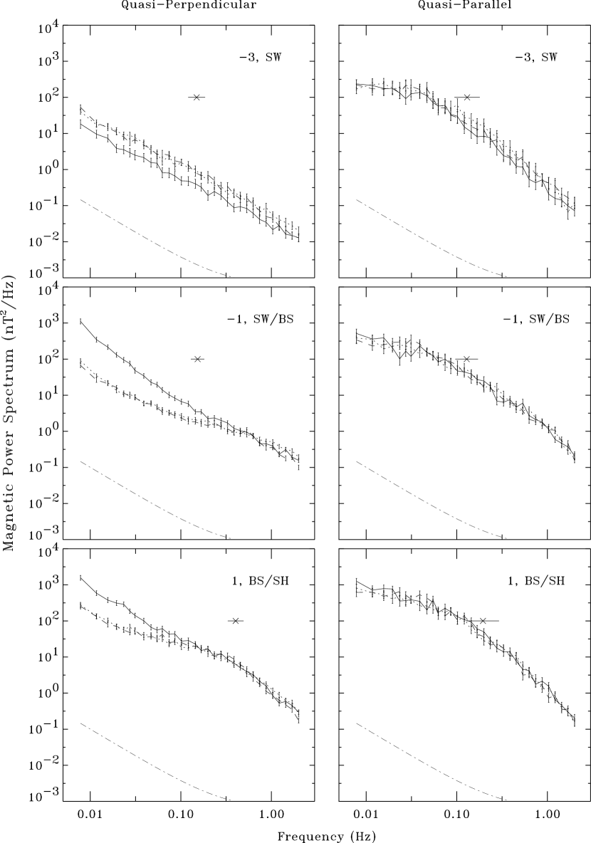
Figure 4: Superposed-epoch analysis of magnetic spectra of 92 quasi-perpendicular (left) and 40 quasi-parallel bow shock crossings (right) from 3 min upstream to 1 min downstream. Solid line: compressive component, dashed line: left hand polarized component, dotted line: right hand polarized component. The cross with the horizontal error bar marks the proton cyclotron frequency. The acronyms SW, BS, SH mean solar wind, bow shock, and magnetosheath, respectively.

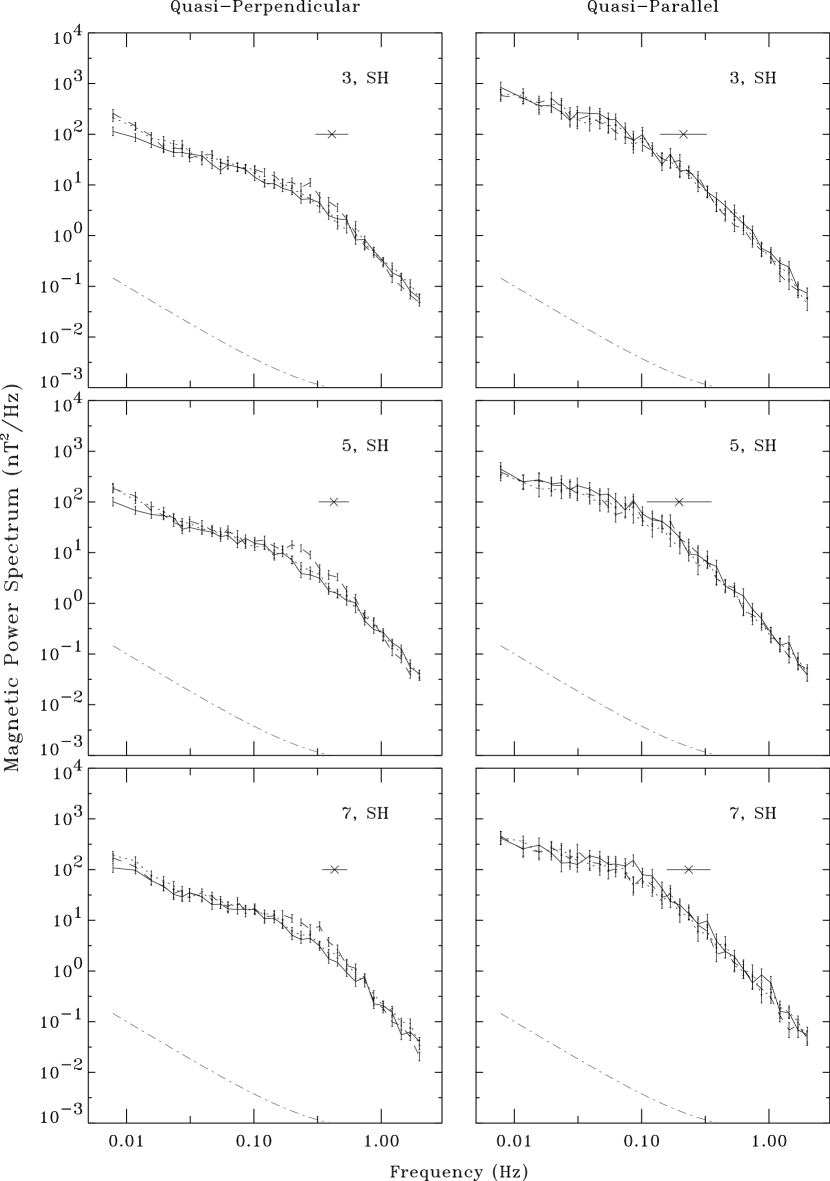
Figure 5: Superposed-epoch analysis of magnetic spectra of 92 quasi-perpendicular (left) and 40 quasi-parallel bow shock crossings (right) from 3 min to 7 min downstream. Same format as Fig. 4.

3.2 Low frequency magnetic fluctuations

In order to analyze the low frequency magnetic fluctuations we perform a spectral analysis of the magnetic field using a cosine-bell filter [see, e.g., Bauer et al., 1995]. The Fourier transform is taken over a time interval of 4 min. Fig. 4 and Fig. 5 show the resulting power spectra of the compressive and the right- and left-hand polarized modes, respectively. In each graph the center time (-3,-1,1,3,5,7) of the transformed time interval is given in minutes relative to crossing time. A cross marks the proton cyclotron frequency $f_{cp}=eB/2\pi m_{p}$ with $m_{p}$ the proton mass. The solar wind (SW) spectrum of Fig. 4, 3 min upstream of the quasi-perpendicular bow shock, shows a structureless decrease to higher frequencies following the power law $S\sim f^{-1.3}$. The compressive mode lies below the transverse modes that represent Alfvén waves frequently observed in the interplanetary medium. They are thought to have their origin in the vicinity of the Sun [Belcher & Davis, 1971]. The spectrum upstream of the quasi-parallel bow shock has much more power than that upstream of the quasi-perpendicular bow shock. It also has a different structure: For lower frequencies it shows a flatter decrease ($S\sim f^{-0.5}$), while for higher frequencies it decreases more steeply ($S\sim f^{-2.0}$). The kink in the spectrum lies below the proton cyclotron frequency.

The next power spectra (-1, SW/BS) contain magnetic field data from the upstream region and the bow shock itself. At the quasi-perpendicular bow shock the compressive mode at low frequencies is one order of magnitude higher compared to the transverse modes and follows a power law of $S\sim f^{-2.1}$. This represents simply the spectrum of the jump of the magnetic field across the shock filtered with a cosine bell function. The spectra of the transverse modes are a little higher than 2 min earlier and the decrease with frequency is not constant any more. At the quasi-parallel bow shock the increase of the magnetic field is not visible, which is not surprising since the magnetic field increases only gradually. Level and structure of the spectrum are similar to those calculated 2 min earlier.

The spectra (1, SW/BS) contain magnetic field data from again the bow shock itself and from the magnetosheath just downstream of the bow shock. At the quasi-perpendicular bow shock the compressive mode behaves similar to the spectrum 2 min earlier, whereas the spectral power of the transverse modes is higher than 2 min earlier. Just below the proton cyclotron frequency first indications of a plateau are visible. At the quasi-parallel bow shock wave activity is significantly enhanced by a factor of 4 compared to the upstream spectra. Again all three modes behave similar. The proton cyclotron frequencies increase according to the magnetic field increase by a factor of 3 at the quasi-perpendicular bow shock and by a factor of 2 at the quasi-parallel bow shock.

Figure 5 shows that for both categories of shock crossings the spectra do not change much in the interval 2 to 8 min downstream of the bow shock. Below $f_{cp}$ the compressive and the right-hand polarized modes downstream of the quasi-perpendicular bow shock follow a power law $S\sim f^{-1.1}$, whereas the spectral energy of the left-hand polarized mode is clearly enhanced in the frequency interval from about 0.1 Hz to about the proton cyclotron frequency. This fact is investigated more carefully in Section 4. Downstream of the quasi-parallel bow shock the spectral energy is again higher than downstream of the quasi-perpendicular bow shock. For $f<f_{cp}$ it follows the power law $S\sim f^{-0.8}$. 3 min after the crossing the spectral energy is higher than in the 2 later spectra but already lower than directly at the bow shock. For both categories the spectral energy decreases steeply ($S\sim f^{-2.6}$) for $f>f_{cp}$.

3.3 Discussion

The processes in the bow shock transition region itself cannot be described in terms of magnetohydrodynamics (MHD). However, if one considers the bow shock as an infinitesimally thin discontinuity one can derive from the MHD equations the Rankine-Hugoniot jump conditions (see, e.g., Siscoe, 1983), which are relations for the conditions in the plasma upstream and downstream of the discontinuity under the assumption of time independence.

For mass continuity the jump condition is

$$n_{2}v_{n2}-n_{1}v_{n1}=0$$ (3)

where the subscripts 1 and 2 denote the upstream and downstream values of the corresponding parameters, respectively. According to Eq. (3) the product of the downstream-to-upstream ratio of the electron density $N_{e}$ and the normal proton velocity $v_{n}$, which is equivalent to the plasma bulk speed normal to the discontinuity, must be unity. For the quasi-parallel events this product is observed to be about 0.6. This fact is not surprising, since the considered upstream time profiles are not taken from the quiet solar wind regime but from the dynamic foreshock region, which is highly time dependent. For the quasi-perpendicular events this product is observed to be about 0.8, which means that the jump condition Eq. (3) is not fully satisfied. This could be explained by the fact that we have not measured the exact electron density, but only the density of electrons with energies between 15 eV and 30 keV. Electrons with higher energies are negligible since already in the energy range of 1.8 - 30 keV the upstream density is of the order of $10^{-5}$ cm^-3. However, particularly in the cold solar wind, electrons with energies below the instrument cut-off contribute an essential part to the total electron density. Therefore we use the corrected electron density $N_{e}^{*}$. The correction is calculated with the assumption of a Maxwellian distribution of the measured temperature. However, as has been measured, e.g., recently by the Wind spacecraft [Fig. 4 of Lin, 1997], the quiet solar wind flow cannot be described by a single Maxwellian distribution over its whole energy range. Therefore the electron density could easily be overestimated by the correction, especially in the cold solar wind regime where the low energy electrons are more important than in the warmer magnetosheath regime. In order to satisfy the jump condition Eq. (3) we can estimate, that the value of the corrected electron density upstream of the quasi-perpendicular bow shock is about 20% too high if we assume that the error in the downstream value is not of importance. Other factors for the apparent deviation from mass continuity could be the unknown bow shock motion, which changes the downstream plasma velocity by a higher percentage than the upstream plasma velocity, and the uncertainty of the shock normal vector.

For an exactly parallel shock wave one derives from the Rankine-Hugoniot jump condition that the magnetic field remains constant in magnitude and direction and one is left with the equations for a purely hydrodynamic shock wave. In the case of an exactly perpendicular shock wave the jump conditions give the relation

$$\frac{n_{2}}{n_{1}}=\frac{B_{2}}{B_{1}}=\frac{v_{1}}{v_{2}}$$ (4)

For the limit of high Mach numbers, i.e., the Alfvén Mach number $M_{A}\rightarrow\infty$ and the sonic Mach number $M_{s}\rightarrow\infty$, Eq. (4) has a value of 4 for $\gamma=5/3$. Since we do not observe the extreme cases of exactly perpendicular and exactly parallel geometry but quasi-perpendicular and quasi-parallel shock wave crossings with finite Mach numbers the numbers given above are not reached. For the quasi-perpendicular bow shock the ratio Eq. (4) is about 3 for the average magnetic field $B$ and proton normal velocity $v_{n}$, and somewhat less for the corrected electron density $N_{e}^{*}$ according to the above mentioned probable overestimation of this parameter in the solar wind regime. For the quasi-parallel bow shock the change in the magnitude of the magnetic field is significantly lower than for the quasi-perpendicular bow shock, which is consistent with theory.

In their study of subcritical quasi-perpendicular shocks, Thomsen et al., [1985] found that the downstream electron temperature is nearly isotropic, $T_{e\perp 2}/T_{e\|2}\approx 0.9$ , and that the downstream-to-upstream ratio $T_{e\perp 2}/T_{e\perp 1}$ of the perpendicular temperature is approximately equal to the ratio $B_{2}/B_{1}$ of the magnetic field strength. From the latter result they concluded that the net heating is adiabatic, although $T_{e\perp}/B$ is not constant. Obtaining averages, $T_{e\perp 2}/T_{e\|2}\approx 0.9$, $T_{e\perp 2}/T_{e\perp 1}\approx 2.6$, and $B_{2}/B_{1}\approx 3.0$, we can confirm these results for our data set of (subcritical and supercritical) quasi-perpendicular shocks. Moreover, isotropy of the downstream electron temperature and adiabatic net heating is also found for our data set of quasi-parallel shocks, for which we obtain averages $T_{e\perp 2}/T_{e\|2}\approx 1.0$, $T_{e\perp 2}/T_{e\perp 1}\approx 1.7$, and $B_{2}/B_{1}\approx 1.8$.

An interesting question of shock physics is how the dissipated bulk flow energy of the solar wind is partitioned amongst ion and electron heating. For the average proton-to-electron temperature ratio we found $T_{p}/T_{e}\approx 6$ downstream of the quasi-parallel bow shock and $T_{p}/T_{e}\approx 4$ downstream of the quasi-perpendicular bow shock. Hence, for quasi-parallel shocks proton heating is more favored with respect to electron heating than for quasi-perpendicular shocks.

Let us turn to the low frequency waves of Fig. 4 and Fig. 5. At quasi-parallel bow shocks the wave power observed 3 min upstream of the keytime is much higher than the power of the interplanetary Alfvén waves observed upstream of quasi-perpendicular shocks. This enhanced power reflects upstream waves generated in the foreshock. Observations of upstream waves have recently been reviewed by Greenstadt et al. [1995] and Russell & Farris [1995]. The nonlinear steepening of the shock leads to whistler precursors phase standing in the shock frame. The interaction between ions reflected at the shock and the incoming solar wind can drive ion beam instabilities. These are probably the source of large-amplitude waves observed at periods around 30 s. Finally, there are upstream propagating whistlers with frequencies around 1 Hz, which seem to be generated directly at the shock. The most striking feature in the average spectrum of upstream waves observed 3 min before the keytime is the kink at $0.04\,{\rm Hz}\approx f_{cp}/3$. The average power measured in the flat portion 0.01–0.04 Hz of the spectrum corresponds to a mean square amplitude $\delta B_{1}\approx 4\,nT$ or $\delta B_{1}/B\approx 0.4$. Large-amplitude waves observed in this frequency range [Le & Russell, 1992; Blanco-Cano & Schwartz, 1995] have been interpreted as upstream propagating magnetosonic waves excited by the right-hand resonant ion beam instability, upstream propagating Alfvén/ion cyclotron waves excited by the left-hand resonant ion beam instability, or downstream propagating magnetosonic waves excited by the non-resonant instability. Whereas the upstream propagating magnetosonic waves should be left-hand polarized in the shock frame (and also in the spacecraft frame), the other two wave types should be right-hand polarized. This might explain why none of the two circular polarizations dominates in our average spectra. Moreover, the compressional component is comparable to the two transverse components. This shows that the waves propagate at oblique angles to the magnetic field. For oblique propagation, low frequency waves have only a small helicity [Gary, 1986]. Thus they are rather linearly than circularly polarized.

The power spectra presented by Le & Russell [1992] exhibit clear peaks at $f\approx f_{cp}/3$. Looking into the spectra of individual time intervals, we find that sometimes the IRM data exhibit similar spectral peaks. However, most of the individual spectra do not have clear peaks, but are rather flat in the range 0.01–0.04 Hz like the average spectrum of Fig. 4. The steep decrease of the power above about $f\approx f_{cp}/3$ is common to our spectra and those reported previously. In fact, the maximum growth rate of the ion beam generated waves is expected for frequencies below the proton cyclotron frequency [e.g., Scholer et al., 1997].

In Fig. 2 we saw that magnetic fluctuations above 0.23 Hz in the foreshock have root mean square amplitudes $\delta B_{2}\approx 1.5$ nT. This is comparable to typical amplitudes of the upstream propagating whistlers. In individual time intervals these narrow-band waves lead to clear spectral peaks at frequencies around 1 Hz. However, since the frequency varies from event to event, no such peak appears in the average spectra.

At the keytime of quasi-parallel bow shocks we observed a clear enhancement of the wave power. This enhancement can either be due to an amplification of the upstream waves or due to wave generation at the shock interface. Wave generation at the shock due to the interface instability has been found in hybrid simulations of Winske et al. [1990] and Scholer et al. [1997]. This instability is driven by the interaction between the incoming solar wind ions and the heated downstream plasma at the shock interface. Amplification of upstream waves has been predicted by McKenzie & Westphal [1969] who analyzed the transmission of MHD waves across a fast shock. They found that the amplitude of Alfvén waves increases by a factor of 3. For compressional waves the amplification can even be stronger. However, the hybrid simulations of Krauss-Varban [1995] show that the transmission of waves across the shock is complicated by mode conversion.

The proton temperature anisotropy downstream of the quasi-perpendicular bow shock serves as a source of free energy. According to both observations and simulations this kind of free energy drives two modes of low frequency waves under the plasma conditions in the magnetosheath: the ion cyclotron wave and the mirror mode (see e.g., Sckopke et al., 1990, Hubert et al., 1989 and Anderson et al., 1994 for observations, Price et al., 1986, and Gary et al., 1993 for simulations, and Schwartz et al. 1996 for a review).

Which of these waves grow under which conditions is investigated in Section 4, where we divide the crossings of quasi-perpendicular shocks into cases with low and high upstream $\beta$, respectively. It turned out that for this classification by $\beta$ the differences become somewhat clearer than for a classification by upstream Mach number. The critical Mach number $M^{*}$ above which ion reflection is required to provide the necessary dissipation is strongly dependent on the plasma-$\beta$ [Edmiston & Kennel, 1984]. We have calculated the ratio $M_{ms}/M^{*}$ for our shock crossings and have found that all subcritical shocks are low-$\beta$, i.e., that the classification low-$\beta$ versus high-$\beta$ is more or less identical to the classification subcritical versus supercritical. The reason for this is that $M^{*}\rightarrow 1$ for $\beta\gg 1$. As the excitation of mirror and ion cyclotron waves depends on $\beta$, the results of Section 4 should be interpreted as the effect of the plasma-$\beta$ and not as an effect of subcritical or supercritical Mach numbers.

For the quasi-parallel bow shocks, we could not investigate the difference between subcritical and supercritical shocks, because no subcritical quasi-parallel shock was identified in the data set. Trying higher thresholds for the division into low and high Mach numbers, we did not find any qualitative differences. In this context it should be noted that only one of the cases in our data set has an Alfvén Mach number in the range $M_{A}\leq 2.3$, for which quasi-parallel shocks are steady according to the hybrid simulations of Krauss-Varban & Omidi [1991].

4 Comparison of quasi-perpendicular low-$\beta$ and high-$\beta$ bow shock crossings

In order to reveal the origin of the left-hand polarized component in the power spectra downstream of the quasi-perpendicular bow shock (Fig. 5) we divide the crossings into classes with low ($<0.5$) and high ($>1.0$) upstream $\beta$ and compare these two classes. There are 20 low-$\beta$ and 47 high-$\beta$ cases. The crossings with $0.5\leq\beta\leq 1.0$ are not included in this analysis in order to emphasize the differences between the low-$\beta$ and high-$\beta$ regimes.

Figure 6: Superposed-epoch analysis of the plasma parameter $\beta$, the proton temperature anisotropy $T_{p\perp}/T_{p\|}$, and the mirror instability criterion from 2 min upstream to 4 min downstream of the quasi-perpendicular bow shock (BS) on the left for 20 low-$\beta$, on the right of 47 high-$\beta$ crossings.

4.1 Plasma and magnetic field parameters

In Fig. 6 we show some interesting differences between the low-$\beta$ and high-$\beta$ categories. Of course the plasma parameter $\beta$ differs essentially. In the upstream region $\beta$ is derived by setting the proton density to the corrected electron density and the proton temperature to $10^{-5}$ K, the long term average of the proton temperature, since proton distribution functions are not well measured in the cold solar wind (Section 3.1). The classification for the low-$\beta$ and high-$\beta$ categories is derived from the estimated plasma $\beta$ in the upstream region. The first panel of Fig. 6 shows that the same classification could be obtained using the plasma-$\beta$ of the downstream region with the limits shifted to larger values. The most striking differences between the low-$\beta$ and high-$\beta$ bow shock are shown in the next two panels, i.e., the proton temperature anisotropy $T_{p\perp}/T_{p\|}$ and the mirror wave instability criterion. Both parameters are again determined only in the downstream region. The instability criterion for almost perpendicular propagation of the mirror mode in its general form [Hasegawa, 1969] is given by

$$-1+\sum_{j}\beta_{j\perp}\left(\frac{\beta_{j\perp}}{\beta_{j\|}}-1\right)>0.$$ (5)

The subscript $j$ denotes the particle species ($j$ = $e$, $p$ for electrons and protons, respectively).

Downstream of the quasi-perpendicular low-$\beta$ bow shock the proton temperature anisotropy is very high, $T_{p\perp}/T_{p\|}\approx 2.5$, immediately behind the shock and remains high, $T_{p\perp}/T_{p\|}>2$, throughout the whole magnetosheath interval investigated. Downstream of the quasi-perpendicular high-$\beta$ bow shock the proton temperature anisotropy is also significant, but lower compared to the low-$\beta$ bow shock, i.e., $T_{p\perp}/T_{p\|}\approx 1.8$ just behind the bow shock and $T_{p\perp}/T_{p\|}\approx 1.3$ further downstream. The mirror instability criterion is only marginally satisfied immediately downstream of the quasi-perpendicular low-$\beta$ bow shock and is not satisfied at later times, since the instability criterion does not only depend on the particle temperature anisotropy but also on the absolute value of $\beta$. Downstream of the quasi-perpendicular high-$\beta$ bow shock the mirror instability criterion is satisfied in the entire interval of 4 min behind the shock. Extremely high values of the left-hand side of Eq. (5) are occasionally observed immediately behind the shock.

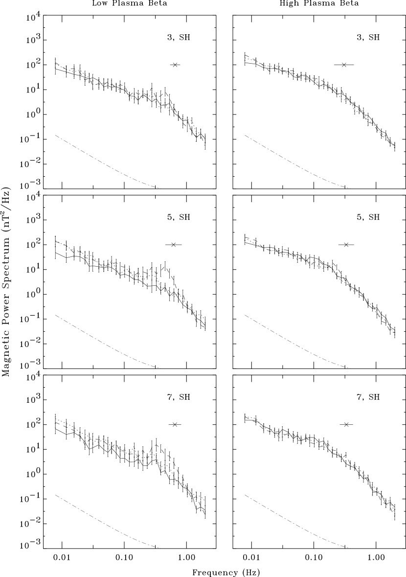
Figure 7: Superposed-epoch analysis of magnetic power spectra downstream of 20 quasi-perpendicular low-$\beta$ and 47 quasi-perpendicular high-$\beta$ bow shock crossings. Same format as Fig. 5.

4.2 Low frequency magnetic fluctuations

Fig. 7 shows the magnetic power spectra downstream of the quasi-perpendicular low-$\beta$ (left) and high-$\beta$ (right) bow shock, 3, 5, and 7 min after the crossing time. Now it becomes obvious that the left-hand polarized mode dominates only behind the quasi-perpendicular bow shock with low-$\beta$ in a frequency interval below the proton cyclotron frequency. 5 and 7 min downstream, the left-hand polarized mode has up to one order of magnitude more power spectral density than the compressive and the right-hand polarized components. Below the frequency range where the left-hand polarized component dominates in the low-$\beta$ cases, the spectrum downstream of the quasi-perpendicular high-$\beta$ bow shock shows a weaker gradient than downstream of the low-$\beta$ bow shock. In addition, the compressive mode lies on the same level as the transverse modes and occasionally at somewhat higher levels, whereas 5 and 7 min downstream of the low-$\beta$ bow shock the compressive mode lies clearly below the transverse modes.Due to the higher magnetic field the proton cyclotron frequency is a factor of about 2.3 higher downstream of the low-$\beta$ bow shock ($B\approx$ 45 nT) than downstream of the high-$\beta$ bow shock ($B\approx$ 23 nT).

At this point, let us collect some numbers for typical wave amplitudes. For that purpose we use the root mean square amplitude $\delta B_{2}$ given in Eq. (2), which has already been shown in Fig. 2 and can be obtained by integrating the power spectra for frequencies above 0.23 Hz, and we use the root mean square amplitude $\delta B_{1}$ of fluctuations in the frequency range 0.01–0.04 Hz. The range 0.01–0.04 Hz has been chosen, because it corresponds to the flat portion of the spectrum observed 3 min upstream of the keytime of quasi-parallel bow shocks. These upstream waves have $\delta B_{1}\approx 4$ nT or $\delta B_{1}/B\approx 0.4$. In contrast, the Alfvén waves seen in the solar wind upstream of quasi-perpendicular bow shocks have $\delta B_{1}\approx 0.8$ nT or $\delta B_{1}/B\approx 0.09$. At the keytime of quasi-parallel bow shocks we observed a clear enhancement of the wave power, which leads to $\delta B\approx 8$ nT or $\delta B/B\approx 0.5$.

In this section we saw that the characteristics of the wave activity downstream of quasi-perpendicular shocks depend on $\beta$. For low $\beta$, the magnetic fluctuations above 0.23 Hz are dominated by left-hand polarized fluctuations with $\delta B_{2}\approx 3$ nT or $\delta B_{2}/B\approx 0.08$, which will be interpreted as ion cyclotron waves. For high $\beta$, typical amplitudes are $\delta B_{2}\approx 1.5$ nT or $\delta B_{2}/B\approx 0.08$.

4.3 Discussion

Sckopke et al. [1990] have performed a case study of low-$\beta$ subcritical bow shock crossings, using the AMPTE/IRM data of September 5, and November 2, 1984. These events are also included in our quasi-perpendicular low-$\beta$ data set: There are 8 events from September 5 and 3 events from November 2, 1984. Sckopke et al. [1990] identified the dominating left-hand polarized component with the ion cyclotron wave which can be generated by a proton temperature anisotropy (e.g., Hasegawa, 1975). The growth rate of the ion cyclotron wave is positive when the instability criterion is satisfied. This holds for the resonance with protons when

$$\frac{T_{p\perp}}{T_{p\|}}>\frac{f_{cp}}{f_{cp}-f}.$$ (6)

The AMPTE/IRM plasma instrument did not resolve ion masses, therefore all ions are assumed to be protons.

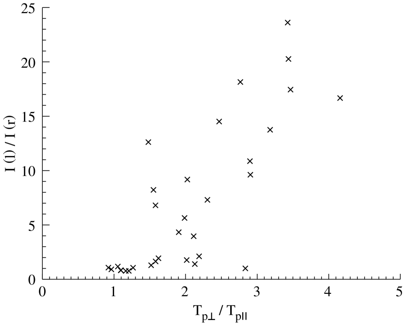
Figure 8: Ratio of the left-hand polarized to the right hand polarized component $I(l)/I(r)$ against the proton temperature anisotropy $T_{p\perp}/T_{p\|}$ ot 32 2-min intervals from 4 to 8 min downstream of the quasi-perpendicular low-$\beta$ bow shock.

Figure 8 shows the ratio of the left-hand polarized to the right-hand polarized component in the frequency band 0.3–$0.8f_{cp}$ for 32 2-min intervals from 4 to 8 min downstream of the quasi-perpendicular low-$\beta$ bow shock as a function of the proton temperature anisotropy. There is a clear correlation found between these two ratios with a correlation coefficient of 0.8. This shows that the wave intensity more than 4 min downstream of the quasi-perpendicular bow shock depends strongly on the local temperature anisotropy.

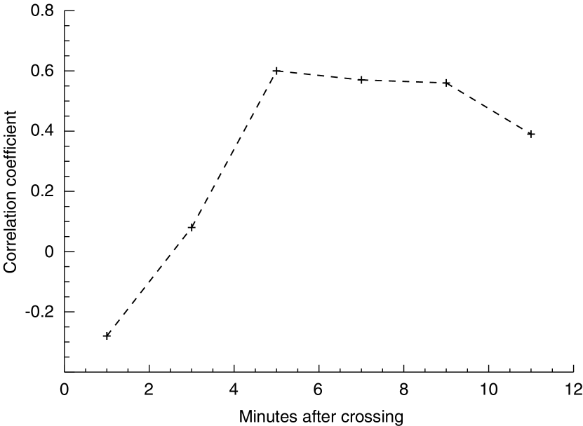
Figure 9: Temporal evolution of the correlation coefficient of the ratios $I(l)/I(r)$ and $T_{p\perp}/T_{p\|}$ downstream of the quasi-perpendicular low-$\beta$ bow shock.

The temporal evolution of the correlation coefficients, calculated for 2-min intervals downstream of the quasi-perpendicular low-$\beta$ bow shock, is shown in Fig. 9. The value of the correlation coefficient 11 minutes downstream is not reliable since only a limited data set extends so far downstream. Although the temperature anisotropy is highest immediately downstream of the bow shock, the best correlation is found around 5 min downstream. This shows that the ion cyclotron waves need a certain time to develop in the moving plasma.

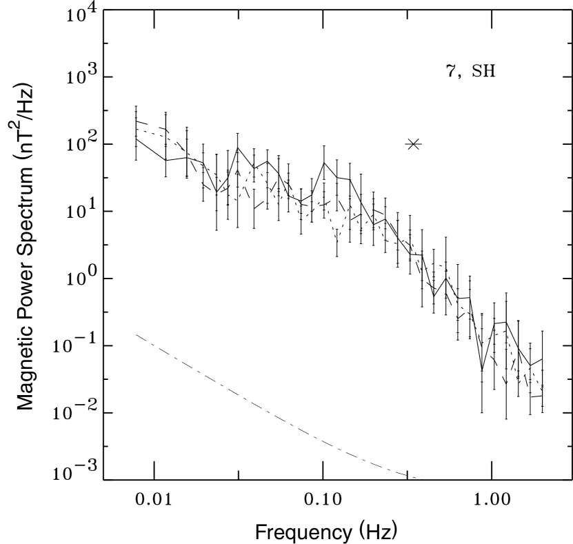
Figure 10: Superposed-epoch analysis of magnetic spectra 7 min downstream of 9 quasi-perpendicular high-$\beta$ bow shock crossings of which the mirror instability criterion is well satisfied.

Since downstream of the quasi-perpendicular high-$\beta$ bow shock the mirror instability criterion is satisfied on average, we have looked more carefully for this highly compressive non-propagating mode. The fact that the compressive mode has a higher power spectral density downstream of the high-$\beta$ than downstream of the low-$\beta$ shock might indicate the existence of mirror modes. We therefore perform a superposed epoch analysis for 9 cases for which the mirror instability criterion is particularly well satisfied, 7 min downstream of the high-$\beta$ bow shock. The resulting spectrum is shown in Fig. 10. In this spectrum we find a compressive mode slightly dominating at some frequencies well below the proton cyclotron frequency.

Contrary to the correlation of the intensity of the left-hand polarized ion cyclotron waves to the proton temperature anisotropy for quasi-perpendicular low-$\beta$ cases, our investigation does not reveal a clear correlation of the intensity of the compressive mode to any parameter for the quasi-perpendicular high-$\beta$ cases. One reason for this could be that the highly compressive mirror mode, which is expected to exist under the observed high-$\beta$ conditions is a purely growing mode with frequencies being pure Doppler-shifted frequencies. Consequently, the waves do not appear in a fixed frequency interval and can be smeared out in the superposition. Therefore we have looked into the individual spectra of intervals 5, 7, and 9 min downstream of the quasi-perpendicular high-$\beta$ bow shock when the mirror criterion is fulfilled. This is the case in 34 of the quasi-perpendicular high-$\beta$ events (72 %). Only in 4 cases (12 % of the quasi-perpendicular high-$\beta$ events where the mirror criterion is fulfilled) mirror waves can clearly be identified in the magnetosheath and are visible in several consecutive spectra. These events and the means of identification of the mirror modes are described in Czaykowska et al. [1998]. The 4 events have in common that the angle $\theta_{Bn}$ is larger than $80^{\circ}$. But there are also almost perpendicular high-$\beta$ events with large values of the left-hand side of Eq. (5) where no indication for mirror waves is visible. Thus a more complex dependence on different parameters seems to determine the growth of the mirror wave. For 14 of the high-$\beta$ events (41 %) where the mirror instability criterion is fulfilled, the compressive component is at least slightly dominating at several frequencies. Several of these events have an angle $\theta_{Bn}<80^{\circ}$. In addition, 2 high-$\beta$ events show ion cyclotron waves in the consecutive spectra taken 5, 7, and 9 min downstream. It is well known [Price et al., 1986; Gary et al., 1993] that the growths of the ion cyclotron and mirror waves are competing processes. In the magnetosheath plasma the crucial parameters for this competition are the $\alpha$-particle concentration and the plasma-$\beta$. However, in our data set we have found many events in the high-$\beta$ regime where none of the two wave modes can be identified although the proton temperature anisotropy is high. This seems to indicate that the dominance of the growing mode does not persist long enough to be visible in one spectrum. The energy of the growing mode might be transferred to other modes by nonlinear effects.

Statistical studies of measurements in the magnetosheath suggest that a relation of the form

$$\frac{T_{p\perp}}{T_{p\|}}-1=\frac{S}{(\beta_{p\|})^{\alpha}}$$ (7)

exists between the proton temperature anisotropy and the ratio $\beta_{p\|}$ of field-aligned proton pressure and magnetic pressure. Analyzing AMPTE/CCE data, Anderson et al. [1994] determined $S=0.85$ and $\alpha=0.48$ and Fuselier et al. [1994] determined $S=0.83$ and $\alpha=0.58$. Using AMPTE/IRM data, Phan et al. [1994] obtained $S=0.58$ and $\alpha=0.53$. We performed a similar analysis on our data set of quasi-perpendicular bow shock crossings. For this analysis we computed 2-min averages of all measurements of $T_{p\perp}/T_{p\|}$ and $\beta_{p\|}$ taken between the keytime and 8 min downstream of the keytime. We find a reasonable fit to Eq. (7) with $S=0.43\pm 0.03$ and $\alpha=0.58\pm 0.05$, which is not too different from the result of Phan et al. [1994].

A relation of the form of Eq. (7) is regarded as the consequence of the combined action of ion cyclotron and mirror waves, which grow due to the temperature anisotropy and reduce this anisotropy by means of pitch angle scattering. The growth of the waves depends on $T_{p\perp}/T_{p\|}$ and $\beta_{p\|}$ and it is expected that the anisotropy is reduced until the growth rate, $\gamma_{m}$, of the most unstable wave falls below some threshold. In fact, Anderson et al. [1994] showed that Eq. (7) with their values of $S$ and $\alpha$ corresponds approximately to the threshold $\gamma_{m}/2\pi f_{cp}=0.01$. Hence, the validity of Eq. (7) indicates that the magnetosheath plasma reaches a state near marginal stability of the waves driven by the temperature anisotropy. As noted above, we found that data obtained less than 8 min downstream of quasi-perpendicular bow shocks satisfy a relation of the form Eq. (7) with values of $S$ and $\alpha$ that are not too different from those determined by Phan et al. [1994] for the entire magnetosheath. This indicates that the state near marginal stability is already reached close to the shock.

Figure 7 shows that the largest amplitudes of the ion cyclotron waves at quasi-perpendicular low $\beta$ shocks are observed on average about 5 min downstream of the keytime (see also Fig. 9). The bow shock moves relative to the spacecraft at speeds of 10–100 km/s. Taking a typical speed of 30 km/s, we can translate 5 min to a downstream distance of 9000 km. According to Fig. 2, the plasma velocity, $v_{pn}$, normal to quasi-perpendicular shock is 120 km/s on average. Thus the plasma needs about 75 s to flow 9000 km downstream. Since the ion cyclotron waves are convected with the plasma while they are growing, these 75 s can serve as a rough estimate for the time $\tau$ that the waves need to reach their maximum amplitudes and saturate. In terms of gyro-periods, we have $\tau\sim 75\,{\rm s}\approx 50/f_{cp}$. Moreover, we find that on the same time scale $\tau$ the temperature anisotropy is reduced from about 2.5 immediately downstream of the low $\beta$ shock to about 2.1 (Fig. 6) and that the ion cyclotron waves typically reach amplitudes of $\delta B/B\sim 0.07$.

These results can be compared with two-dimensional hybrid simulations of McKean et al. [1994]. These authors examined a plasma with $\beta_{p\|}=1$ and $T_{p\perp}/T_{p\|}=3$. Under these conditions the ion cyclotron mode is found to be the dominant mode and the waves saturate after $\tau\approx 5/f_{cp}$ and reach amplitudes of $\delta B/B\sim 0.15$. The proton temperature anisotropy is reduced on the same time scale $\tau$ from 3 to about 1.8. For our data set of low $\beta$ bow shocks $T_{p\perp}/T_{p\|}$ is on average 2.5 and $\beta_{p\|}$ is on average 0.5 immediately downstream of the shock. Since these values are considerably lower than the initial values used by McKean et al. [1994], the plasma simulated by McKean et al. [1994] is initially much farther away from the state of marginal stability. Thus it is not surprising that the waves grow faster, reach larger amplitudes and therefore lead to a stronger reduction of the anisotropy by means of pitch angle scattering.

McKean et al. [1994] also examined a plasma with $\beta_{p\|}=4$ and $T_{p\perp}/T_{p\|}=3$. Under these conditions the ion cyclotron mode dominates for low $\alpha$-particle concentration, whereas the mirror mode dominates for high $\alpha$-particle concentration. The waves saturate after $\tau\approx 10/f_{cp}$ and reach amplitudes of $\delta B/B\sim 0.2$. The proton temperature anisotropy is reduced on the same time scale $\tau$ from 3 to about 1.5. This can be compared with data obtained at the quasi-perpendicular high $\beta$ shock. For our data set of high-$\beta$ bow shocks $T_{p\perp}/T_{p\|}$ is on average 1.8 and $\beta_{p\|}$ is on average 5 immediately downstream of the shock. Again, the plasma simulated by McKean et al. [1994] is initially much farther away from the state of marginal stability. Fig. 6 shows that a reduction of the anisotropy to 1.3 is observed 30 s downstream of the keytime. This can again be translated to a downstream distance and used to estimate the time span that passes while the plasma travels this distance. This estimate gives $8\,{\rm s}\approx 2.5/f_{cp}$. Finally, it should be noted that the mirror waves analyzed by Czaykowska et al. [1998] have amplitudes of $\delta B/B\sim 0.2$, which is comparable to those found in the simulations of McKean et al. [1994].

5 Conclusions

We have analyzed the plasma and magnetic field parameters as well as low frequency magnetic fluctuations at 132 dayside AMPTE/IRM bow shock crossings. The average distance of the subsolar point, which results from the coordinates of the investigated bow shock crossings, is considerably smaller than in other studies, even when normalized to the average solar wind dynamical pressure. A reason for this discrepancy might be a variation of the polytropic index with the solar cycle since our observations are performed during typical solar minimum conditions. The position of the Earth’s bow shock still seems to be a matter of discussion.

A superposed epoch analysis has been carried out by averaging particle and magnetic field data as well as low frequency magnetic spectra upstream and downstream of the bow shock. We have performed this analysis by dividing the events into different categories, i.e., quasi-perpendicular and quasi-parallel events as well as quasi-perpendicular low-$\beta$ and high-$\beta$ events.

The particle and magnetic field data show that upstream of the quasi-parallel bow shock, in the foreshock region, the plasma is already heated compared to the undisturbed solar wind. Moreover, there are more energetic protons in the foreshock region, and the magnetic field is highly variable. Downstream of the quasi-perpendicular bow shock, a proton temperature anisotropy is found, which is higher on average downstream of the quasi-perpendicular low-$\beta$ than downstream of the quasi-perpendicular high-$\beta$ bow shock.

Concerning the low frequency magnetic fluctuations we find that upstream of the quasi-perpendicular bow shock the solar wind spectrum is undisturbed with transverse Alfvén waves surpassing the compressive spectral component. Upstream of the quasi-parallel bow shock largely enhanced wave activity is detected in the turbulent foreshock region. These upstream waves are convected downstream, experiencing an enhancement at the bow shock itself. Downstream of the quasi-perpendicular bow shock the observed proton temperature anisotropy leads to the generation of left-hand polarized ion cyclotron waves under low-$\beta$ conditions and in some cases to the generation of mirror waves under high-$\beta$ conditions. A clear correlation has been observed between the intensity of the left-hand polarized component of the magnetic power spectrum relative to the right-hand polarized component and the proton temperature anisotropy. On the other hand, we could not find a simple correlation between the intensity of the compressive component and any single plasma or magnetic field parameter. In cases where mirror waves are obviously observable mostly three conditions are fulfilled: the plasma-$\beta$ is high, the mirror instability criterion is satisfied and the angle $\theta_{Bn}$ is large, i.e., $\theta_{Bn}\gtrsim 80^{\circ}$. But there are also cases where all these conditions are well satisfied but no mirror waves are visible in the frequency interval under consideration.

References

- (1)
- (2) Anderson, B. J., & S. A. Fuselier, Magnetic pulsations from 0.1 to 4.0 Hz and associated plasma properties in the Earth’s subsolar magnetosheath and plasma depletion layer, J. Geophys. Res. 98, 1461–1479, 1993.
- (3)
- (4) Anderson, B. J., S. A. Fuselier, S. P. Gary, & R. E. Denton, Magnetic spectral signatures in the Earth’s magnetosheath and plasma depletion layer, J. Geophys. Res. 99, 5877–5891, 1994.
- (5)
- (6) Bauer, T. M., W. Baumjohann, R. A. Treumann, N. Sckopke, & H. Lühr, Low-frequency waves in the near-Earth plasma sheet, J. Geophys. Res. 100, 9605-9617, 1995.
- (7)
- (8) Bauer, T. M., Particles and fields at the dayside low-latitude magnetopause, MPE Report 267, Garching, 1997.
- (9)
- (10) Bavassano-Cattaneo, M. B., C. Basile, G. Moreno, & J. D. Richardson, Evolution of mirror structures in the magnetosheath of Saturn from the bow shock to the magnetopause, J. Geophys. Res. 103, 11,961-11,972, 1998.
- (11)
- (12) Belcher, J. W. & L. Davis, Large-amplitude Alfvén waves in the interplanetary medium, 2, J. Geophys. Res. 76, 3534-3563, 1971.
- (13)
- (14) Blanco-Cano, X. & S. J. Schwartz, AMPTE-UKS observations of low frequency waves in the ion foreshock, Adv. Space Res., 15(8/9), 97–101, 1995.
- (15)
- (16) Burgess, D., Cyclical behavior of quasi-parallel collisionless shocks, Geophys. Res. Lett. 16, 345-349, 1989.
- (17)
- (18) Czaykowska, A., T. M. Bauer, R. A. Treumann, & W. Baumjohann, Mirror waves downstream of the quasi-perpendicular bow shock, J. Geophys. Res. 103, 4747-4753, 1998.
- (19)
- (20) Edmiston, J. P., & C. F. Kennel, A parametric survey of the first critical Mach number for a fast MHD shock, J. Plasma Phys., 32, 429-441, 1984.
- (21)
- (22) Fairfield, D. H., Average and unusual locations of the Earth’s magnetopause and bow shock, J. Geophys. Res. 76, 6700–6716, 1971.
- (23)
- (24) Fairfield, D. H., Global aspects of the Earth’s magnetopause, in Magnetospheric Boundary Layers, ed. by B. Battrick, pp. 5-13, ESA, Noordwijk, 1979.
- (25)
- (26) Formisano, V., Orientation and shape of the Earth’s bow shock in three dimensions, Planet. Space Sci., 27, 1151-1161, 1979.
- (27)
- (28) Fuselier, S. A., B. J. Anderson, S. P. Gary, & R. E. Denton, Ion anisotropy/beta correlations in the Earth’s quasi-parallel magnetosheath, J. Geophys. Res. 99, 14,931–14,936, 1994.
- (29)
- (30) Gary, S. P., Low-frequency waves in a high-beta collisionless plasma: Polarization, compressibility and helicity, J. Plasma Phys., 35, 431–447, 1986.
- (31)
- (32) Gary, S. P., S. A. Fuselier, & B. J. Anderson, Ion anisotropy instabilities in the magnetosheath, J. Geophys. Res. 98, 1481–1488, 1993.
- (33)
- (34) Greenstadt, E. W. & M. M. Mellott, Plasma wave evidence for reflected ions in front of subcritical shocks: ISEE 1 and 2 observations, J. Geophys. Res. 92, 4730–4734, 1987.
- (35)
- (36) Greenstadt, E. W., G. Le, & R. J. Strangeway, ULF waves in the foreshock, Adv. Space Res., 15(8/9), 71–84, 1995.
- (37)
- (38) Gurnett, D. A., Plasma waves and instabilities, in Collisionless Shocks in the Heliosphere: Reviews of Current Research, Geophys. Monogr. Ser., 35, ed. by B. T. Tsurutani & R. G. Stone, pp. 207–224, AGU, Washington, DC, 1985.
- (39)
- (40) Hasegawa, A., Drift mirror instability in the magnetosphere, Phys. Fluids, 12, 2642–2650, 1969.
- (41)
- (42) Hasegawa, A., Plasma Instabilities and Nonlinear Effects, Springer-Verlag, New York, 1975.
- (43)
- (44) Hoppe, M. M., C. T. Russell, L. A. Frank, T. E. Eastman, & E. W. Greenstadt, Upstream hydromagnetic waves and their association with backstreaming ion populations: ISEE 1 and 2 observations, J. Geophys. Res. 86, 4471-4492, 1981.
- (45)
- (46) Hubert, D., C. Perche, C. C. Harvey, C. Lacombe, & C. T. Russell, Observation of mirror waves downstream of a quasi-perpendicular shock, Geophys. Res. Lett. 16, 159–162, 1989.
- (47)
- (48) Kennel, C. F., J. P. Edmiston, & T. Hada, A quarter century of collisionless shock research, in Collisionless Shocks in the Heliosphere: A Tutorial Review, Geophys. Monogr. Ser., 34, ed. by R. G. Stone & B. T. Tsurutani, pp. 1-36, AGU. Washington, D.C., 1985.
- (49)
- (50) Krauss-Varban, D., Waves associated with quasi-parallel shocks: Generation, mode conversion and implications, Adv. Space Res., 15(8/9), 271-284, 1995.
- (51)
- (52) Krauss-Varban, D., & N. Omidi, Structure of medium Mach number quasi-parallel shocks: Upstream and downstream waves, J. Geophys. Res. 96, 17,715–17,731, 1991.
- (53)
- (54) Le, G., & C. T. Russell, A study of ULF wave foreshock morphology – II: Spatial variation of ULF waves, Planet. Space Sci., 40, 1215–1225, 1992.
- (55)
- (56) Lee, L. C., C. P. Price, C. S. Wu, & M. E. Mandt, A study of mirror waves generated downstream of a quasi-perpendicular shock, J. Geophys. Res. 93, 247–250, 1988.
- (57)
- (58) Lin, R. P, Observations of the 3D distributions of thermal to near-relativistic electrons in the interplanetary medium by the Wind spacecraft, in Coronal physics from radio and space observations, LNP 483, ed. by Trottet, G., Springer-Verlag, New York, 1997.
- (59)
- (60) Lühr, H., N. Klöcker, W. Oelschlägel, B. Häusler, & M. Acuña, The IRM fluxgate magnetometer, IEEE Trans. Geosci. Remote Sens., GE-23, 259–261, 1985.
- (61)
- (62) McKean, M. E., D. Winske, & S. P. Gary, Two-dimensional simulations of ion anisotropy instabilities in the magnetosheath, J. Geophys. Res. 99, 11,141–11,153, 1994.
- (63)
- (64) McKenzie, J. F., & K. O. Westphal, Transmission of Alfvén waves through the Earth’s bow shock, Planet. Space Sci., 17, 1029–1037, 1969.
- (65)
- (66) Mellott, M. M., & W. A. Livesey, Shock overshoots revisited, J. Geophys. Res. 92, 13,661–13,665, 1987.
- (67)
- (68) Omidi, N., How the bow shock does it, Rev. Geophys., Supplement, 629-637, 1995.
- (69)
- (70) Paschmann, G., H. Loidl, P. Obermayer, M. Ertl, R. Laborenz, N. Sckopke, W. Baumjohann, C. W. Carlson, & D. W. Curtis, The plasma instrument for AMPTE/IRM, IEEE Trans. Geosci. Remote Sens., GE-23, 262–266, 1985.
- (71)
- (72) Paschmann, G., W. Baumjohann, N. Sckopke, & H. Lühr, Structure of the dayside magnetopause for low magnetic shear, J. Geophys. Res. 98, 13,409–13,422, 1993.
- (73)
- (74) Peredo, M., J. A. Slavin, E. Mazur, & S. A. Curtis, Three-dimensional position and shape of the bow shock and their variation with Alfvénic, sonic and magnetosonic Mach numbers and interplanetary magnetic field orientation, J. Geophys. Res. 100, 7907–7916, 1995.
- (75)
- (76) Phan, T.-D., G. Paschmann, W. Baumjohann, N. Sckopke, & H. Lühr, The magnetosheath region adjacent to the dayside magnetopause: AMPTE/IRM observations, J. Geophys. Res. 99, 121–141, 1994.
- (77)
- (78) Price, C. P., D. W. Swift, & L.-C. Lee, Numerical simulations of nonoscillatory mirror waves at the Earth’s magnetosheath, J. Geophys. Res. 91, 101–112, 1986.
- (79)
- (80) Russell, C. T., & M. H. Farris, Ultra low frequency waves at the Earth’s bow shock, Adv. Space Res., 15(8/9), 285–296, 1995.
- (81)
- (82) Scholer, M., H. Kucharek, & V. Jayanti, Waves and turbulence in high Mach number nearly parallel collisionless shocks, J. Geophys. Res. 102, 9821–9833, 1997.
- (83)
- (84) Schwartz, S. J., D. Burgess, & J. J. Moses, Low-frequency waves in the Earth’s magnetosheath: Present status, Ann. Geophys., 14, 1134–1150, 1996.
- (85)
- (86) Sckopke, N., G. Paschmann, S. J. Bame, J. T. Gosling, & C. T. Russell, Evolution of ion distributions across the nearly perpendicular bow shock: Specularly and nonspecularly reflected ions, J. Geophys. Res. 88, 6121–6136, 1983.
- (87)
- (88) Sckopke, N., G. Paschmann, A. L. Brinca, C.W. Carlson, & H. Lühr, Ion thermalization in quasi-perpendicular shocks involving reflected ions, J. Geophys. Res. 95, 6337–6352, 1990.
- (89)
- (90) Siscoe, T. H., Solar system magnetohydrodynamics, in Solar-Terrestrial Physics, ed. by R. L. Carovillano & J. M. Forbes, pp 11-100, Reidel Publishing, Dordrecht, 1983.
- (91)
- (92) Spreiter, J. R., A. L. Summers, & A. Y. Alksne, Hydrodynamic flow and the magnetosphere, Planet. Space Sci., 14, 223-253, 1966.
- (93)
- (94) Stone, R. G., & B. T. Tsurutani (eds.), Collisionless shocks in the Heliosphere: A tutorial review, Geophys. Monogr. 34, AGU, Washington D.C., 1985.
- (95)
- (96) Tsurutani, B. T., & R. G. Stone (eds.), Collisionless shocks in the Heliosphere: Review of current research, Geophys. Monogr. 35, AGU, Washington D.C., 1985.
- (97)
- (98) Thomsen, M. F., J. T. Gosling, & S. J. Bame, Ion and electron heating at collisionless shocks near the critical Mach number, J. Geophys. Res. 90, 137-148, 1985.
- (99)
- (100) Winske, D., N. Omidi, K. B. Quest, & V. A. Thomas, Re-forming supercritical quasi-parallel shocks, 2, Mechanism for wave generation and front re-formation, J. Geophys. Res. 95, 18,821–18,832, 1990.
- (101)
- (102) Winterhalter, D., E. J. Smith, M. E. Burton, N. Murphy, & D. J. McComas, The heliospheric plasma sheet, J. Geophys. Res. 99, 6667-6680, 1994.
- (103)