QUADRUPOLE MISALIGNMENTS AND STEERING IN LONG LINACS

Abstract

We present a study of orbit jitter and emittance growth in a long linac caused by misalignment of quadrupoles. First, assuming a FODO lattice, we derive analytical formulae for the RMS deviation of the orbit and the emittance growth caused by random uncorrelated misalignments of all quadrupoles. We then consider an alignment algorithm based on minimization of BPM readings with a given BPM resolution and finite mover steps.

1 Introduction

In this paper we study the emittance dilution of a beam caused by quadrupole misalignments in a long linac. To suppress the beam break-up instability an energy spread is usually introduced in the beam. For the Next Linear Collider (NLC) [1], the rms energy spread within the bunch will be of order of 1%. Due to the lattice chromaticity, the deflection of the beam by displaced quadrupoles results in the dilution of the phase space and the growth of the projected emittance.

The effect of lattice misalignments has been previously studied in many papers. A qualitative analysis and main scalings were obtained in Ref. [2], and detailed studies with intensive computer simulations are described in Refs. [3, 4, 5]. The purpose of this paper is to develop a simple model based on a FODO lattice approximation for the linac which allows an analytic calculation of the emittance dilution. The model can be also generalized, to include a slow variation of the lattice parameters, as well as variation of both beam energy and the energy spread [6].

Throughout this paper we assume that the number of quadrupoles in the linac is large, $N\gg 1$, and neglect terms of the relative order of $N^{-1}$ in the calculations. For future linear colliders with the center of mass energy in the range of 1 TeV, typically $N\sim 10^{3}$, and $N^{-1}$ is indeed a small number.

2 Beam Orbit in Misaligned Lattice

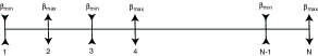
Figure 1: FODO lattice of a linac. Beam positions are measured at the center of each quadrupole.

Let us consider a FODO lattice with a cell length $l$ and a phase advance $\mu$ per cell, consisting of $N$ thin quadrupoles as shown in Fig. 1. The focal length of the quadrupoles is equal to $\pm F$ where the positive and negative values of $F$ refer to the focusing and defocusing quadrupoles respectively. The beam is injected in the linac at the center of the first quadrupole, at $s=0$, with the zero offset and angle, and the beam emittance is measured at the center of the last, $N$th, quadrupole. For the beam position (horizontal or vertical) at the locations of the quadrupoles we will use the notation $x_{1},x_{2},\ldots,x_{N-1},x_{N}$, and the orbit angle at the center of the $k$th quadrupole is denoted by $x^{\prime}_{k}$. The initial conditions for the orbit are $x_{1}=x^{\prime}_{1}=0$. Note that due to our choice of positions, the derivative of the beta function, and hence the Twiss parameter $\alpha$, at all locations 1 through $N$, are equal to zero.

We now assume that each quadrupole in the lattice is misaligned in the transverse direction relative to the axis of the linac by $\xi_{i}$, ($1\leq i\leq N$), where $\xi_{i}$ are random, uncorrelated numbers. Due to the deflection by misaligned quadrupoles, the original straight orbit will be perturbed. The offset $x_{i}$ can be found as

$$x_{i}=\sum_{k<i}R_{ik}\theta_{k},$$ (1)

where $R_{ik}$ is the $(1,2)$ element of the transfer matrix $R$ and $\theta_{i}$ is the deflection angle resulting from the offset of the $i$th quadrupole, $\theta_{i}=\pm\xi_{i}/F$, for the focusing and defocusing quadrupoles. We have $R_{ik}=\sqrt{\beta_{i}\beta_{k}}\sin\Delta\psi_{ik}$, where the betatron phase advance $\Delta\psi_{ik}$ between $k$th and $i$th quadrupoles ($k<i$) is $\Delta\psi_{ik}=(1/2)(i-k)\mu$.

We will also need the orbit angles $x_{i}^{\prime}$ where the prime denotes the derivative with respect to the longitudinal coordinate $s$. For $x_{i}^{\prime}$ we have

$$x_{i}^{\prime}=\sum_{k\leq i}G_{ik}\theta_{k},$$ (2)

where $G_{ik}$, is the $(2,2)$ element of the transfer matrix, $G_{ik}=\sqrt{\beta_{k}/\beta_{i}}\cos\Delta\psi_{ik}$, (note that, due to our choice, $\alpha_{i}=0$).

3 RMS value for the beam offset

To characterize the deviation of the orbit from the linac axis, we will calculate the average value $\langle x_{N}^{2}\rangle$, where the angular brackets denote averaging over all possible values of $\xi$. We assume that the average offset $\langle\xi_{i}\rangle$ vanishes, hence $\langle x_{N}\rangle=0$.

For the lattice shown in Fig. 1 the deflection angle $\theta_{k}$ due to the misaligned $k$th quadrupole is given by $\theta_{k}=(-1)^{k}\xi_{k}/F$, and the beam offset at the end of the linac is

$$x_{N}=\sum_{k=1}^{N-1}R_{Nk}(-1)^{k}\frac{\xi_{k}}{F}.$$ (3)

For the variance of $x_{N}$ we have

$$\langle x_{N}^{2}\rangle=\frac{\langle\xi^{2}\rangle}{F^{2}}\sum_{l=1}^{N-1}R_{Nl}^{2},$$ (4)

where we have used $\langle\xi_{k}\xi_{l}\rangle=\langle\xi^{2}\rangle\delta_{kl}$, with $\langle\xi^{2}\rangle$ being the variance of the random variables $\xi_{i}$. To calculate the sum in Eq. (4), one can average $R_{Nl}^{2}$ over the betatron phase value $R_{Nl}^{2}\rightarrow\frac{1}{4}\beta_{N}\beta_{l}$. One finds,

$$\frac{\langle x_{N}^{2}\rangle}{\beta_{N}}=\frac{N\langle\xi^{2}\rangle}{4F^{2}}(\beta_{\max}+\beta_{\min})=4N\frac{\langle\xi^{2}\rangle}{l}\tan\frac{\mu}{2}.$$ (5)

We see that the rms value $\langle x_{N}^{2}\rangle^{1/2}$ scales as $N^{1/2}$, which is a characteristic feature of the random walk motion.

In a similar fashion, one can find the rms angular spread orbits $\langle{x^{\prime}}_{N}^{2}\rangle^{1/2}$ at the end of the linac. Starting from the general expression

$$x^{\prime}_{N}=\sum_{k=1}^{N}G_{Nk}(-1)^{k-1}\frac{\xi_{k}}{F},$$ (6)

and performing the same averaging as for derivation of Eq. (5), one finds $\langle{x^{\prime}}_{N}^{2}\rangle=\langle x_{N}^{2}\rangle/\beta_{N}^{2}$, where $\langle{x}_{N}^{2}\rangle$ is given by Eq. (5).

4 Chromatic Emittance Growth

When the beam has a nonzero energy spread, due to the chromaticity of the lattice, the misalignments cause an effective emittance growth of the beam [2]. We will calculate the emittance increase, assuming that the beam energy $E$ and the relative energy spread in the beam $\delta$ are constant. We will also assume that the resulting emittance growth is much smaller than the initial emittance of the beam. In this case, we can use the following formula for the final emittance growth

$$\Delta\epsilon = \frac{1}{2}\left[\beta_{N}^{-1}\langle(\Delta x-\langle\Delta x\rangle)^{2}\rangle_{\xi\delta}\right.$$ (7)

$$+ \left.\beta_{N}\langle(\Delta x^{\prime}-\langle\Delta x^{\prime}\rangle)^{2}\rangle_{\xi\delta}\right],$$

where $\Delta x$ and $\Delta x^{\prime}$ are the spread in the coordinate and the angle within the bunch at the and of the linac, and the angular brackets with the subscript ${\xi\delta}$ denote a double averaging: first, averaging over the random misalignment of the quadrupoles and then averaging over the energy distribution function in the beam. We will assume that the energy spread in the beam $\delta$ is so small, that one can use a linear approximation for calculation of $\Delta x$ and $\Delta x^{\prime}$, $\Delta x=\delta\cdot x_{N\delta}\equiv\delta\cdot\partial x_{N}/\partial\delta$ and $\Delta x^{\prime}=\delta\cdot x^{\prime}_{N\delta}\equiv\delta\cdot\partial x^{\prime}_{N}/\partial\delta$. Since $\langle\xi_{i}\rangle=0$, hence $\langle\Delta x\rangle=\langle\Delta x^{\prime}\rangle=0$. In this approximation Eq. (7) reduces to

$$\Delta\epsilon=\frac{1}{2}\overline{\delta^{2}}\left(\beta_{N}^{-1}\left\langle x_{N\delta}^{2}\right\rangle+\beta_{N}\left\langle{x^{\prime}}_{N\delta}^{2}\right\rangle\right),$$ (8)

where $\overline{\delta^{2}}$ is the variance of the energy spread within the beam.

To calculate $x_{N\delta}$ and $x^{\prime}_{N\delta}$ we need to take the derivatives of Eqs. (3) and (6) with respect to $\delta$. For a long linac, the dominant contribution to $\Delta\epsilon$ comes from the dependence of the phase advance $\Delta\psi_{ik}$ versus energy, so we need to differentiate only $\sin\Delta\psi_{ik}$ (or $\cos\Delta\psi_{ik}$) terms in the sum. Calculation gives

$$\beta_{N}^{-1}\left\langle x_{N\delta}^{2}\right\rangle=\beta_{N}\left\langle{x^{\prime}}_{N\delta}^{2}\right\rangle=\frac{4}{3}N^{3}\frac{\langle\xi^{2}\rangle}{l}\tan^{3}\frac{\mu}{2}\,.$$ (9)

which gives for the emittance dilution

$$\Delta\epsilon=\frac{4}{3}\overline{\delta^{2}}N^{3}\frac{\langle\xi^{2}\rangle}{l}\tan^{3}\frac{\mu}{2}\,.$$ (10)

As we see, the increase in the emittance scales with the number of quadrupoles as $N^{3}$.

In the above derivation, to find the dispersion of the beam at the end of the linac, we explicitly differentiated Eq. (3) with respect to the energy. One can use another formula for computing $\partial x_{N}/\partial\delta$ [6],

$$\frac{\partial x_{N}}{\partial\delta}=\sum_{k=1}^{N-1}R_{Nk}(-1)^{k}\frac{x_{k}-\xi_{k}}{F},$$ (11)

that takes into account that the dispersion is generated due to the offset of the particle relative to the center of the quadrupole, and propagates downstream with the same matrix element $R_{Nk}$.

5 Very long linac

Increasing the length of the linac and the number of quadrupoles $N$ brings us to the regime where Eq. (10) is not valid any more. The transition occurs when the phase advance over the length of the linac due to the energy variation $\delta$ becomes comparable to $\pi/2$, $N\delta\cdot d\mu/d\delta\sim\pi/2$. In this case, the differential approximation $\Delta x=\delta\cdot\partial x_{N}/\partial\delta$ that was used in Section 4 is not valid any more, and the scaling $\Delta\epsilon\propto N^{3}$ breaks down.

We can estimate the emittance dilution in this regime, using the following arguments. Let us denote by $l_{c}$ the decoherence length in the linac such that $(l_{c}/l)\delta\cdot d\mu/d\delta\sim\pi/2$ ($l$ is the FODO cell length). When the beam passes the distance $l_{c}$, due to filamentation, the betatron oscillations of the beam are converted into the increased emittance, and the subsequent motion becomes uncorrelated with the previously excited betatron oscillations. The emittance growth on the distance $l_{c}$ is given by Eq. (10), in which $N=2l_{c}/l$,

$$\Delta\epsilon_{c}=\frac{4}{3}\overline{\delta^{2}}\left(\frac{2l_{c}}{l}\right)^{3}\frac{\langle\xi^{2}\rangle}{l}\tan^{3}\frac{\mu}{2}\approx\frac{\langle\xi^{2}\rangle}{l\sqrt{\overline{\delta^{2}}}}\,.$$ (12)

The total emittance increase in the linac of length $l_{L}$ in this regime is equal to $\Delta\epsilon_{c}$ multiplied by the number of coherent distances $l_{L}/l_{c}$ in the linac

$$\Delta\epsilon=\Delta\epsilon_{c}\frac{l_{L}}{l_{c}}\sim\frac{l_{L}\langle\xi^{2}\rangle}{l^{2}\tan\frac{\mu}{2}}\sim\frac{N\langle\xi^{2}\rangle}{l\tan\frac{\mu}{2}}\,.$$ (13)

Note that if the linac length $l_{L}<l_{c}$, the emittance dilution is reversible in principle – the initial beam emittance can be recovered by taking out the dispersion generated by the misaligned quadrupoles downstream of the linac. For very long linacs, when $l_{L}>l_{c}$, the emittance growth becomes irreversible due to the phase space filamentation.

6 Alignment with account of BPM errors and finite mover steps

Measuring the beam position at each quadrupole, with the knowledge of the lattice functions, allows us to find the quadrupole offsets $\xi_{i}$. Moving the quadrupoles by distance $-\xi_{i}$ would position them in the original state, and restore the ideal lattice. Of course, in reality, there are many factors, such as wakefields and measurement errors, that do not allow to perfectly align the lattice. Here we will study two such effects: errors associated with the BPM measurements, and finite step of the quadrupole movers.

Consider first the effect of BPM errors. Due to the finite resolution of BPMs the measured vector of the beam transverse offsets $X^{M}=(x_{1}^{M}\ldots x_{N}^{M})$ differs from the exact values $X=(x_{1}\ldots x_{N})$ by an error vector $e$, $X^{M}=X+e$, where $e=(e_{1}\ldots e_{N})$. The errors are small relative to the measured values, $|e_{i}|\ll|x_{i}|$. We assume that the BPMs are built in the quadrupoles, and the quadrupole displacement $\xi_{k}$ also moves the center line of the BMP, so that BPM reading is $x_{k}^{M}=x_{k}-\xi_{k}+e_{k}$. Using the measured offsets $x_{k}^{M}$ we infer the quadrupole offsets $\zeta_{k}$ from the following equation

$$x_{i}^{M}+\zeta_{i}=\sum_{k=1}^{i-1}R_{ik}(-1)^{k}\frac{\zeta_{k}}{F}.$$ (14)

Note that without errors, $e_{k}=0$, we would find from Eq. (14) the correct value $\zeta_{k}=\xi_{k}$. Measurement errors $e_{k}$ cause the inferred values of the offsets differ from the true ones, $\zeta_{k}\neq\xi_{k}$.

We then align the lattice by moving the quadrupoles by distance $-\zeta_{k}$. After the alignment the corrected beam orbit $\tilde{x}_{i}$ does not vanish:

$$\tilde{x}_{i} = \sum_{k=1}^{i-1}R_{ik}(-1)^{k}\frac{\xi_{k}-\zeta_{k}}{F}$$ (15)

$$= x_{i}-x^{M}_{i}-\zeta_{i}=-e_{i}+\xi_{i}-\zeta_{i}.$$

Since the quadrupoles after alignment are located at $\xi_{k}-\zeta_{k}$, the beam offset relative to the center of the quadrupole, $\tilde{x}_{k}-(\xi_{k}-\zeta_{k})$, is equal to $-e_{k}$. This allows us to use Eq. (11) to find the emittance dilution in the linac after the alignment,

$$x_{N\delta}=-\sum_{k=0}^{N-1}R_{Nk}(-1)^{k-1}\frac{e_{k}}{F}.$$ (16)

Assuming that $e_{k}$ are uncorrelated random numbers makes the problem equivalent to the orbit equation (3) with the result given by Eq. (5),

$$\beta_{N}^{-1}\left\langle x_{N\delta}^{2}\right\rangle=4N\frac{\langle e^{2}\rangle}{l}\tan\frac{\mu}{2}.$$ (17)

We see that the rms value of the dispersion at the and of the linac after alignment scales as $\sqrt{N}$. Calculating in a similar way the variance of the derivative $x^{\prime}_{N\delta}$, gives the chromatic emittance growth after alignment,

$$\Delta\epsilon=4N\overline{\delta^{2}}\frac{\langle e^{2}\rangle}{l}\tan\frac{\mu}{2}\,.$$ (18)

Let us now assume that in addition to the BPM errors the quadrupole movers have a finite step so that the final position of the quadrupoles $\zeta_{k}$ after alignment is $\xi_{k}-\zeta_{k}+r_{k}$, where as above, $\zeta_{k}$ is the offset inferred from the measurements (and containing BPM errors), and $r_{k}$ is the quadrupole movement error. Again, we assume that $r_{k}$ are random, uncorrelated numbers, and of course uncorrelated with the BPM errors $e_{k}$. For the beam orbit after alignment we now have

$$\tilde{x}_{i}=-e_{i}+\xi_{i}-\zeta_{i}+\sum_{k=1}^{i-1}R_{ik}r_{k}$$ (19)

with the resulting emittance growth that is a combination of Eqs. (18) and (10),

$$\Delta\epsilon=4N\overline{\delta^{2}}\frac{\langle e^{2}\rangle}{l}\tan\frac{\mu}{2}+\frac{4}{3}\overline{\delta^{2}}N^{3}\frac{\langle r^{2}\rangle}{l}\tan^{3}\frac{\mu}{2}\,.$$ (20)

From this equation, it follows that for a large $N$, the contribution of the movers errors becomes more important and imposes tighter tolerances on the movers.

References

• [1] The NLC Design Group, Report SLAC-474, SLAC, Stanford, CA, USA (May 1996).
• [2] R.Β D. Ruth, in US/CERN Joint Topical Course on β€œFrontiers of Particle Beams” (1987), pp. 440–460.
• [3] T.Β O. Raubenheimer and R.Β D. Ruth, Nucl. Instrum. Meth. A302, 191 (1991).
• [4] A.Β Sery and O.Β Napoly, Phys. Rev. E53, 5323 (1996).
• [5] A.Β Sery and A.Β Mosnier, Phys. Rev. E56, 3558 (1997).
• [6] G. V. Stupakov, to be published.
• [7] R.Β Assmann et al., Tech. Rep. SLAC-AP-103, SLAC (April 1997).