On electromagnetic induction

Giuseppe Giuliani
Dipartimento di Fisica ‘Volta’, Via Bassi 6, 27100 Pavia, Italy
Email: giuliani@fisav.unipv.it
Web site - http://matsci.unipv.it/percorsi/

Abstract. A general law for electromagnetic induction phenomena is derived from Lorentz force and Maxwell equation connecting electric field and time variation of magnetic field. The derivation provides with a unified mathematical treatment the statement according to which electromagnetic induction is the product of two independent phenomena: time variation of magnetic field and effects of magnetic field on moving charges. The general law deals easily - without ad hoc assumptions - with typical cases usually considered as exceptions to the flux rule and contains the flux rule as a particular case.

1 Introduction

It is, in general, acknowledged that the theoretical treatment of electromagnetic induction phenomena presents some problems when part of the electrical circuit is moving. Some authors speak of exceptions to the flux rule; others save the flux rule by ad hoc choices of the integration line over which the induced $emf$ is calculated. Several attempts to overcome these difficulties have been made; a comprehensive one has been performed by Scanlon, Henriksen and Allen. However, their treatment - as others - fails to recognize that one must distinguish between the velocity of the circuit elements and the velocity of the electrical charges (see section 2 below). Therefore, these authors reestablish the flux rule and, consequently, do not solve the problems posed by its application.

Since 1992, I have been teaching electromagnetism in a course for Mathematics students and I had to deal with the problems outlined above. I have found that it is possible to get a general law for electromagnetic induction that contains the standard flux rule as a particular case.

The matter has conceptual relevance; it has also historical and epistemological aspects that deserve to be investigated. Therefore, it is, perhaps, worthwhile to submit the following considerations to the attention of a public wider than that of my students.

2 A general law for electromagnetic induction

Textbooks show a great variety of positions about how the flux rule can be applied to the known experimental phenomena of electromagnetic induction. Among the more lucid approaches, let us refer to the treatment given by Feynman, Leighton and Sands in the Feynman Lectures on Physics. They write:

In general, the force per unit charge is $\vec{F}/q=\vec{E}+\vec{v}\times\vec{B}$. In moving wires there is the force from the second term. Also, there is an $\vec{E}$ field if there is somewhere a changing magnetic field. They are two independent effects, but the emf around the loop of wire is always equal to the rate of change of magnetic flux through it.

This sentence is followed by a paragraph entitled Exceptions to the “flux rule”, where the authors treat two cases - the Faraday disc and the ‘rocking plates’ - both characterized by the fact that there is a part of the circuit in which the material of the circuit is changing. As the authors put it, at the end of the discussion:

The ‘flux rule does not work in this case. It must be applied to circuits in which the material of the circuit remain the same. When the material of the circuit is changing, we must return to the basic laws. The correct physics is always given by the two basic laws

$$\vec{F} = e(\vec{E}+\vec{v}\times\vec{B})$$ (1)

$$\nabla\times\vec{E} = -{{\partial\vec{B}}\over{\partial t}}$$ (2)

2.1 A definition of $emf$

In order to try shedding some more light on the subject, let us begin with the acknowledgement that the expression of Lorentz force

$$\vec{F}=q(\vec{E}+\vec{v}\times\vec{B})$$ (3)

not only gives meaning to the fields solutions of Maxwell equations when applied to point charges, but yields new predictions.

The velocity appearing in the expression of Lorentz force is the velocity of the charge: from now on, we shall use the symbol $\vec{v}_{charge}$ for distinguishing the charge velocity from the velocity $\vec{v}_{line}$ of the circuit element that contains the charge. This is a basic point of the present treatment.

Let us consider the integral of $(\vec{E}+\vec{v}_{charge}\times\vec{B})$ over a closed loop:

$${\cal E}=\oint_{l}{(\vec{E}+\vec{v}_{charge}\times\vec{B})\,\cdot\,\vec{dl}}=\oint_{l}{\vec{E}\,\cdot\,\vec{dl}}+\oint_{l}{(\vec{v}_{charge}\times\vec{B})\,\cdot\,\vec{dl}}$$ (4)

This integral yields the work done by the electromagnetic field on a unit positive point charge along the closed path considered. It presents itself as the natural definition of the electromotive force, within the Maxwell - Lorentz theory: $emf={\cal E}$.

Let us now calculate the value of $\cal E$ given by equation (4). The calculation of the first integral appearing in the third member of equation (4) yields:

$$\oint_{l}{\vec{E}\,\cdot\,\vec{dl}}=\int_{S}rot\,\vec{E}\,\cdot\,\hat{n}\,dS=-\int_{S}{{\partial\vec{B}}\over{\partial t}}\,\cdot\,\hat{n}\,dS$$ (5)

where $S$ is any surface having the line $l$ as contour and where we have made use of Maxwell equation (2). The calculation of the last integral of equation (5) yields:

$$\oint_{l}\vec{E}\,\cdot\,\vec{d}l=-{{d}\over{dt}}\int_{S}{\vec{B}\,\cdot\,\hat{n}\,dS}-\oint_{l}(\vec{v}_{line}\times\vec{B})\,\cdot\,\vec{d}l$$ (6)

where $\vec{v}_{line}$ is the velocity of the circuit element $\vec{dl}$. Notice that equation (6) is the result of a theorem of vectorial calculus that is valid for any vector field $\vec{G}$, like the magnetic field, for which $div\,\vec{G}=0$. Therefore, we get:

$${\cal E}=\left[-{{d}\over{dt}}\int_{S}{\vec{B}\,\cdot\,\hat{n}\,dS}-\oint_{l}(\vec{v}_{line}\times\vec{B})\,\cdot\,\vec{d}l\right]+\oint_{l}(\vec{v}_{charge}\times\vec{B})\,\cdot\,\vec{dl}$$ (7)

This equation says that:

1. The induced emf is, in general, given by three terms.

2. The first two - grouped under square brackets for underlining their common mathematical and physical origin - come from the line integral $\oint_{l}{\vec{E}\,\cdot\,\vec{dl}}$, whose value is controlled by Maxwell equation (2) through equation (5). Accordingly, their sum must be zero when the magnetic field does not depend on time. In this case, the law assumes the simple form:

   $${\cal E}=\oint_{l}(\vec{v}_{charge}\times\vec{B})\,\cdot\,\vec{dl}$$ (8)

3. The third term comes from the magnetic component of Lorentz force; we shall see later how this term may be different from zero.

4. The flux rule is contained in the general law as a particular case.

The general law (7) can be written also in terms of the vector potential $\vec{A}$. If we put

$$\vec{E}=-grad\,\varphi-{{\partial\vec{A}}\over{\partial t}}$$ (9)

in the first integral of the third member of equation (4), we get at once

$${\cal E}=-\oint_{l}{{\partial\vec{A}}\over{\partial t}}\cdot\vec{d}l+\oint_{l}(\vec{v}_{charge}\times\vec{B})\,\cdot\,\vec{dl}$$ (10)

since $\oint_{l}{grad\,\varphi\cdot\vec{d}l}=0$. When the magnetic field does not depend on time ($\partial\vec{B}/\partial t=0$), we have:

$$\oint_{l}{\vec{E}\cdot\vec{d}l}=-\oint_{l}{{{\partial\vec{A}}\over{\partial t}}\cdot\vec{d}l}=-\int_{S}{rot\,{{\partial\vec{A}}\over{\partial t}}\cdot\hat{n}\,dS}=0$$ (11)

since $rot\,(\partial\vec{A}/\partial t)=0$, because $\partial\vec{B}/\partial t=0$. Therefore, the only surviving term in the expression of the induced $emf$ is coming from the magnetic component of Lorentz force and the law assumes the form given by equation (8).

2.2 $\vec{A}$ versus $\vec{B}$

Traditionally, textbooks use equations containing the magnetic field in dealing with induction phenomena: the $emf$ in a loop is partially (general law) or totally (flux rule) dependent on a surface integral of $\vec{B}$. The laws are predictive, but they are not causal laws. The values of $\vec{B}$ over the surface of integration cannot be causally related to the value of the $emf$ around the circuit because $\vec{B}$ acts at a distance (with an infinite propagation velocity): in this case, $\vec{B}$ is not a good field, since a good field, in Feynman’s words, can be defined as

…a set of numbers we specify in such a way that what happens at a point depends only on the numbers at that point. We do not need to know any more about what’s going on at other places.

On the contrary, the same equations written in terms of the vector potential, are causal laws since they relate the value of the $emf$ around the circuit to the values of $-\partial\vec{A}/\partial t$ at the points of the loop: the vector potential is, in this case, a good field.

3 How the law works

3.1 General features

Let us come back to the general law (7 or 10). The charge velocity appearing in these equations contributes to build up, through the factor $\vec{v}_{charge}\times\vec{B}$ the induced electromotive field. The charge velocity is given by:

$$\vec{v}_{charge}=\vec{v}_{line}+\vec{v}_{drift}$$ (12)

where $\vec{v}_{drift}$ is the drift velocity.

Therefore, the general equation for electromagnetic induction assumes the form:

$${\cal E} = \left[-{{d}\over{dt}}\int_{S}{\vec{B}\,\cdot\,\hat{n}\,dS}-\oint_{l}(\vec{v}_{line}\times\vec{B})\,\cdot\,\vec{d}l\right]+$$ (13)

$$+ \oint_{l}(\vec{v}_{line}\times\vec{B})\,\cdot\,\vec{dl}+\oint_{l}(\vec{v}_{drift}\times\vec{B})\,\cdot\,\vec{dl}$$

or, in terms of the vector potential:

$${\cal E}=-\oint_{l}{{\partial\vec{A}}\over{\partial t}}\cdot\vec{d}l+\oint_{l}(\vec{v}_{line}\times\vec{B})\,\cdot\,\vec{dl}+\oint_{l}(\vec{v}_{drift}\times\vec{B})\,\cdot\,\vec{dl}$$ (14)

When the circuit is made by a loop of wire, equation (13) reduces to equation

$${\cal E}=\left[-{{d}\over{dt}}\int_{S}{\vec{B}\,\cdot\,\hat{n}\,dS}-\oint_{l}(\vec{v}_{line}\times\vec{B})\,\cdot\,\vec{d}l\right]+\oint_{l}(\vec{v}_{charge/line}\times\vec{B})\,\cdot\,\vec{dl}$$ (15)

and equation (14) to equation

$${\cal E}=-\oint_{l}{{\partial\vec{A}}\over{\partial t}}\cdot\vec{d}l+\oint_{l}(\vec{v}_{charge/line}\times\vec{B})\,\cdot\,\vec{dl}$$ (16)

because the drift velocity is always parallel to the line element $\vec{dl}$ and, consequently, the integral containing it is zero. We have introduced the new notation $v_{charge/line}$ for remembering that we are dealing with the velocity of the charge that, in this case, can be replaced by the velocity of the circuit element that contains it. It is worth stressing again that, when the magnetic field does not depend on time, equation (15) cannot be read in terms of flux variation, since the sum of the first two terms under square brackets is zero as it is the equivalent term of equation (16) containing the time derivative of the vector potential.

When part of the circuit is made by extended material, the calculation of the drift velocity contribution to the induced $emf$ is not an easy task, since the distribution of current lines in the material may be very complicated. In section 3.2.6 and 3.2.7 we shall treat particularly simple cases with a circular symmetry. In all other cases, we shall neglect the drift velocity in the calculation of the induced $emf$ (look at the end of section 3.2.6 for a further discussion of this point).

3.2 How it works in specific cases

We shall now discuss some cases widely treated in literature, in order to see how the general law (and the flux rule) can be applied to specific problems.

3.2.1 When a bar is moving

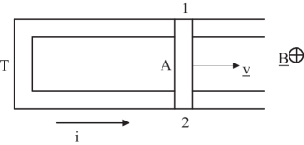
Figure 1: the conducting bar $A$, of length $a$, moves with constant velocity $\vec{v}$ in a uniform and constant magnetic field $\vec{B}$ perpendicular to and entering the page. The bar $A$ slides on the conducting frame $T$. A steady current $i$ circulates in the circuit $T21$.

Let us consider the circuit of fig. 1. The conducting bar $A$, of length $a$, slides with constant velocity $\vec{v}$ over the conducting frame $T$ in a uniform and constant magnetic field $\vec{B}$ perpendicular to the plane of the frame and entering the page: the frame $T$ is at rest with respect to the source of the magnetic field. A steady current flows along the direction indicated in the figure. Notice that in this case we can neglect without approximation the drift velocity of the charge because it is always directed along the integration line (owing to the Hall effect). According to the general law (16), the first integral is zero as zero is sum of the first two terms of equation (15): as a matter of fact, if we choose the counterclockwise direction for the line integral, we obtain for the sum of these two terms:

$$Bav_{line}-Bav_{line}=0$$ (17)

The induced electromotive force is then given by:

$${\cal E}=Bav_{charge/line}$$ (18)

The surviving term is the one coming from the magnetic component of Lorentz force. Moreover, the theory predicts that the emf is localized into the bar: the bar acts as a battery and, as a consequence, between the two points $1$ and $2$ of the frame that are in contact with the bar, one should measure a potential difference given by $V_{1}-V_{2}={\cal E}-ir$, where $i$ is the circulating current and $r$ is the resistance of the bar.

Finally, it is worth stressing that the energy balance shows that the magnetic component of Lorentz force plays the role of an intermediary: the electrical energy dissipated in the circuit comes from the work done by the force that must be applied to keep the bar moving with constant velocity.

Let us now recall how the flux rule deals with this case. It predicts an emf given by $Bav_{line}$. In the light of the general law (15) and of its discussion, we understand why the flux rule predicts correctly the value of the emf: the reason lies in the fact that the two line integrals under square brackets cancel each other. However, we have shown above that the physics embedded in the general equation (15) forbids to read equation (18) as the result of:

$${\cal E}=Bav_{line}+[-Bav_{line}+Bav_{line}]=Bav_{line}$$ (19)

that leaves operative the first term coming from the flux variation.

Before leaving this subject, it is worth saying something about the long debate about the meaning of ‘localized $emf$’. With reference to the moving bar, we can proceed as follows. The points $1$ and $2$ divide the circuit into two parts: the one on the left obeys Ohm law $\Delta V=iR$ and the current enters it at point $1$ at higher potential and leaves it at point $2$ at lower potential; the part on the right does not obeys Ohm law and the current enters it at point $2$ at lower potential and leaves it at point $1$ at higher potential. We say that the $emf$ is localized in the right part of the circuit: it can be experimentally distinguished from the other.

3.2.2 The Faraday disc: 1

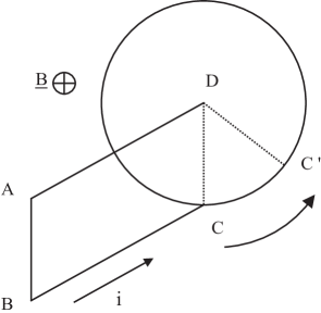
Figure 2: the Faraday disc. A conducting disc rotates with constant angular velocity $\omega$ in a uniform and constant magnetic field $\vec{B}$ perpendicular to and entering the plane of the disc. A conducting frame $DABC$ makes conducting contacts with the center and a point on the periphery of the disc. A steady current $i$ circulates as indicated by the arrow.

A conducting disc is rotating with constant angular velocity $\omega$ in a uniform and constant magnetic field $\vec{B}$ perpendicular to the disc and entering the page (fig. 2). A conducting frame $DABC$ makes conducting contacts with the center and a point on the periphery of the disc. A steady current $i$ circulates as indicated by the arrow.

By applying the general laws (16) or (15) to the integration line at rest $ABCDA$, we see that, if we neglect the contribution of the drift velocity:

• since the magnetic field does not depend on time, the first integral in (16) is zero

• equivalently, the sum of the first two integrals in (15) is zero. In the present case, each of the two terms is zero: the flux associated with the circuit does not change and $\vec{v}_{line}$ is zero everywhere, since the integration line has been chosen at rest

• the only surviving term is the one due to the magnetic component of Lorentz force and its value is given by (we are taking the counterclockwise direction for the line integration):

  $${\cal E}={{1}\over{2}}\omega BR^{2}$$ (20)

  where $R$ is the disc radius. In doing this calculation, we have neglected - as explained at the end of section 3.1, the charge drift velocity (we shall take it into account in section 3.2.7).

Of course, the emf given by equation (20) is induced along any radius, as it can be seen by considering the circuit $ABCC^{\prime}DA$. If the radius $C^{\prime}D$ is considered at rest, the case is the same as that of the circuit $ABCDA$ discussed just before. If the radius $C^{\prime}D$ is considered in motion with angular velocity $\omega$, we see again, both from equation (16) and equation (15), that the only surviving term is the one due to the magnetic component of Lorentz force with the only difference that, now, the first term of equation (15) $({{1}/{2}})\omega BR^{2}$ is cancelled out by the second $-({{1}/{2}})\omega BR^{2}$, due to the movement of the line elements of the radius $DC^{\prime}$; the line elements lying on the $CC^{\prime}$ arc give a null contribution.

Let us now see how the flux rule deals with the Faraday disc. If we choose the lines at rest $ABCDA$ or $ABCC^{\prime}DA$, we find that the induced emf is zero; if we choose the integration line $ABCC^{\prime}DA$, with the radius $C^{\prime}D$ considered in motion, we obtain the correct result ${\cal E}=({{1}/{2}})\omega BR^{2}$.

As in the case of the moving bar, the flux rule gets the correct result only because the two line integrals under square brackets in equation (15) cancel each other. As in the case of the moving bar, the physics embedded in the general equation forbids an interpretation of the mathematical result in terms of flux variation: again the physical origin of the induced emf is due to the intermediacy of the magnetic component of Lorentz force.

3.2.3 The unipolar induction

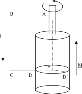
Figure 3: the unipolar induction. A conducting cylindrical magnet rotates about its axis in a counterclockwise direction. A conducting frame $ABCD$ makes conducting contacts between a point on the axis of the magnet and a point on its surface. A steady current $i$ circulates as indicated by the arrow.

The so called unipolar induction is illustrated in fig. 3. When the cylindrical and conducting magnet $M$ rotates about its axis with angular velocity $\omega$ in the counterclockwise direction, a current flows in the circuit as indicated by the arrow. It is easy to see that the discussion of the unipolar induction can be reduced to that of the Faraday disc for both general law and flux rule: the general law applied to the circuit $ABCDEA$ at rest yields an $emf$ induced in the radius $DE$ given by $(1/2)\omega B\overline{DE}^{2}$, while the flux rule applied to the same circuit predicts a zero emf. If one consider instead the integration line $ABCDD^{\prime}EA$ with the radius $D^{\prime}E$ in motion, analogous to the path $ABCC^{\prime}DA$ of fig. 2 concerning the Faraday disc, one can follow the same arguments developed in that case.

3.2.4 The flux varies, but…

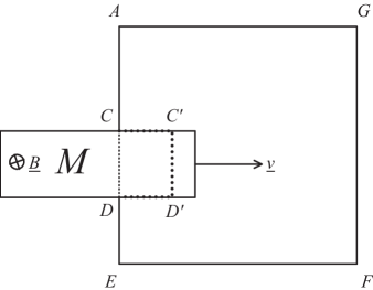
Figure 4: Kaempffer’s example. The circuit $DEFGAC$ is closed by the conducting magnet $M$ that is moving to the right with constant velocity $\vec{v}$. The magnet is sufficiently long in the direction perpendicular to the page so that there is a magnetic field only within the magnet. There is no induced $emf$ in spite of the fact that there is a flux change through the circuit at rest $ACDEFGA$.

In fig. 4 a case discussed by Scanlon, Henriksen and Allen and originally due to Kaempffer is presented. When the conducting magnet $M$ moves, as indicated, with constant velocity $\vec{v}$, there is no induced $emf$ - if the magnet is sufficiently long in the direction perpendicular to the page so that there is a magnetic field only within the magnet. If we consider the integration line $ACDEFGA$ at rest, there is a flux variation without induced $emf$. Also in this case, we must choose ad hoc the integration line - for instance the line $ACC^{\prime}D^{\prime}DEFGA$, where the segment $C^{\prime}D^{\prime}$ moves with the magnet - if we want to save the flux rule. On the other hand, the general law works well, whatever integration line is chosen.

3.2.5 The ‘rocking plates’

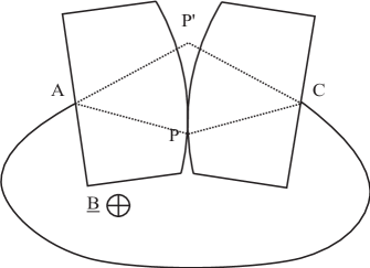
Figure 5: the ‘rocking plates’. Two conducting plates oscillate back and forth in a uniform and constant magnetic field perpendicular to the plates.

This is one of the two ‘exceptions to the flux rule’ discussed by Feynman, Leighton and Sands (fig. 5). The two plates oscillate slowly back and forth so that their point of contact moves from $P$ to $P^{\prime}$ and viceversa. The circuit is closed by a wire that connects point $A$ and $C$. The magnetic field $\vec{B}$ is perpendicular to the plates and enters the page. The authors write:

If we imagine the “circuit” to be completed through the plates on the dotted line shown in the figure, the magnetic flux through this circuit changes by a large amount as the plates are rocked back and forth. Yet the rocking can be done with small motions, so that $\vec{v}\times\vec{B}$ is very small and there is practically no emf.

According to the general law (15) the sum of the first two terms of equation (15) must be zero. Hence:

$$\oint_{l}(\vec{v}_{line}\times\vec{B})\,\cdot\,\vec{d}l=-{{d}\over{dt}}\int_{S}{\vec{B}\,\cdot\,\hat{n}\,dS}$$ (21)

Therefore, the third term of equation (15) coming from the magnetic component of Lorentz force equals the magnetic flux variation changed in sign, if, of course, we assume that the charge velocity can be taken equal to the velocity of the element of conductor that contains it (the drift velocity is neglected). The conclusion is that there is an induced $emf$: its average value is given by $-\Delta\phi/\Delta t$ where $\Delta\phi$ is the flux variation between the two extreme positions of the plates and $\Delta t$ the interval of time taken in going from one position to the other: the induced $emf$ gets smaller and smaller as $\Delta t$ gets larger and larger; when the motion of the plates is very slow, we can conclude with Feynman that ‘there is practically no $emf$’. Notice that the induced $emf$ changes in sign (and the current its direction) when the the rocking motion is reversed.

3.2.6 The Corbino disc

The discussion of this case will show how the charge drift velocity, always neglected before, plays its role in the building up of the induced electromotive field and, therefore, of the induced $emf$. In 1911, Corbino studied theoretically and experimentally the case of a conducting disc with a hole at its center. If a voltage is applied between the inner and the outer periphery of the disc, a radial current will flow, provided that the experimental setup is realized in a way suitable for maintaining the circular symmetry: the inner and outer periphery are covered by highly conducting electrodes; therefore, the inner and outer periphery are two equipotential lines. If a uniform and constant magnetic field is applied perpendicularly to the disc, a circular current will flow in the disc.

The first theoretical treatment of this case is due, as far as I know, to Boltzmann who wrote down the equations of motion of charges in combined electric and magnetic fields. Corbino, apparently not aware of this fact, obtained the same equations already developed by Boltzmann. However, while Boltzmann focused on magnetoresistance effects, Corbino interpreted the theoretical results in terms of radial and circular currents and studied experimentally the magnetic effects due to the latter ones.

The application of the general law of electromagnetic induction to this case leads to the same results usually obtained (as Boltzmann and Corbino did) by writing down and solving the equations of motion of the charges in an electromagnetic field (by taking into account, explicitly or implicitly, the scattering processes).

If $I_{radial}$ is the radial current, the radial current density $J(r)$ will be:

$$J(r)={{I_{radial}}\over{2\pi rs}}$$ (22)

and the radial drift velocity:

$$v(r)_{drift}={{I_{radial}}\over{2\pi rsne}}$$ (23)

where $s$ is the thickness of the disc, $n$ the electron concentration and $e$ the electron charge. In the present case the general law of electromagnetic induction assumes the simple form of equation (8) with $v_{charge}=v_{drift}$; therefore, the induced $emf$ around a circle of radius $r$ is given by:

$${\cal E}_{circular}=\oint_{0}^{2\pi r}{(\vec{v}(r)_{drift}\times\vec{B}})\cdot\vec{dr}={{I_{radial}\,B}\over{sne}}$$ (24)

The circular current $dI(r)_{circular}$ flowing in a circular strip of radius $r$ and section $s\cdot dr$ will be, if $\rho$ is the resistivity:

$$dI_{circular}={{{\cal E}_{circular}\,sdr}\over{\rho\,2\pi r}}={{\mu B}\over{2\pi}}I_{radial}{{{dr}\over{r}}}$$ (25)

and the total circular current:

$$I_{circular}={{\mu B}\over{2\pi}}I_{radial}\ln{{r_{2}}\over{r_{1}}}$$ (26)

where $\mu$ is the electron mobility, $r_{1}$ and $r_{2}$ the inner and outer radius of the disc (we have used the relation $\mu=1/\rho ne$). Equation (26) is the same as that derived and experimentally tested by Corbino.

The power dissipated in the disc is:

$$W=(I^{2}R)_{radial}+(I^{2}R)_{circular}=I_{radial}^{2}R_{radial}(1+\mu^{2}B^{2})$$ (27)

where we have used equation (26) and the two relations:

$$R_{radial} = {{\rho}\over{2\pi s}}\ln{{r_{2}}\over{r_{1}}}$$ (28)

$$R_{circular} = {{\rho^{2}}\over{s^{2}}}{{1}\over{R_{radial}}}$$ (29)

Equation (27) shows that the phenomenon may be described as due to an increased resistance $R_{radial}(1+\mu^{2}B^{2})$: this is the magnetoresistance effect. The circular induced $emf$ is ‘distributed’ homogeneously along each circle. Each circular strip of section $s\cdot dr$ acts as a battery that produces current in its own resistance: therefore, the potential difference between two points arbitrarily chosen on a circle is zero. Hence, as it must be, each circle is an equipotential line.

The above application of the general law yields a description of Corbino disc that combine Boltzmann (magnetoresistance effects) and Corbino (circular currents) point of view and shows how the general law can be applied to phenomena traditionally considered outside the phenomenological domain for which it has been derived.

3.2.7 The Faraday disc: 2

The discussion of Corbino disc helps us in better understanding the physics of the Faraday disc. Let us consider a Faraday disc in which the circular symmetry is conserved. This may be difficult to realize; anyway, it is interesting to discuss it. As shown above, the steady condition will be characterized by the flow of a radial and of a circular current. The mechanical power needed to keep the disc rotating with constant angular velocity $\omega$ is equal to the work per unit time done by the magnetic field on the rotating radial currents. Then, it will be given by:

$$W=\int_{0}^{2\pi}{}\int_{r_{1}}^{r_{2}}({J_{radial}\,r\,d\alpha}\,s)(B\,dr)(\omega\,r)=I_{radial}\,{{1}\over{2}}\,\omega\,B\,(r_{2}^{2}-r_{1}^{2})$$ (30)

where the symbols are the same as those used in the previous section. The point is that the term

$${\cal E}={{1}\over{2}}\,\omega\,B\,(r_{2}^{2}-r_{1}^{2})$$ (31)

is the induced $emf$ due only to the motion of the disc. This $emf$ is the primary source of the induced currents, radial and circular. Therefore, the physics of the Faraday disc with circular symmetry, may be summarized as follows:

1. the source of the induced currents is the induced $emf$ due to the rotation of the disc

2. the primary product of the induced $emf$ is a radial current

3. the drift velocity of the radial current produces in turn a circular induced $emf$ that give rise to the circular current

4 General law and flux rule

The cases discussed above must be considered as illustrative examples. Obviously, the conceptual foundations of the general law and of the flux rule can be discussed without any reference to particular cases. The general law has been already dealt with in great detail. Let us now focus our attention on the flux rule.

Let us define - this, of course, is not our choice - the induced emf as

$${\cal E}=\oint_{l}\vec{E}\cdot\vec{d}l$$ (32)

where $\vec{E}$ obeys Maxwell equations. As shown above (equations 5 - 6), this leads immediately to the conclusion that the induced emf is given by:

$${\cal E}=\oint_{l}\vec{E}\,\cdot\,\vec{d}l=-{{d}\over{dt}}\int_{S}{\vec{B}\,\cdot\,\hat{n}\,dS}-\oint_{l}(\vec{v}_{line}\times\vec{B})\,\cdot\,\vec{d}l$$ (33)

or, in terms of the vector potential, by (equations 10 - 11):

$${\cal E}=\oint_{l}{\vec{E}\cdot\vec{d}l}=-\oint_{l}{{{\partial\vec{A}}\over{\partial t}}\cdot\vec{d}l}$$ (34)

and is always zero when $\partial\vec{B}/\partial t=0$.

Of course, this result is not satisfactory, if we want to save the flux rule. Therefore, one may suggest to define the induced emf as:

$${\cal E}=\oint_{l}\vec{E}\,\cdot\,\vec{d}l+\oint_{l}(\vec{v}_{line}\times\vec{B})\,\cdot\,\vec{d}l=-{{d}\over{dt}}\int_{S}{\vec{B}\,\cdot\,\hat{n}\,dS}$$ (35)

thus reestablishing the flux rule. This is, for instance, the choice made by Scanlon, Henriksen and Allen. However:

• since the velocity appearing in equation (35) is clearly the velocity of the line element $\vec{d}l$, this definition has no physical meaning.

• the definition is ad hoc. As a consequence, as in the paper by Scanlon, Henriksen and Allen, the line of integration must be chosen ad hoc for obtaining predictions in accordance with the experimental findings.

5 Conclusions

The straightforward application of two fundamental laws of electromagnetism – Maxwell equation $rot\vec{E}=-\partial\vec{B}/\partial t$ and Lorentz law $\vec{F}=q(\vec{E}+\vec{v}\times\vec{B})$ – leads to a general law for electromagnetic induction phenomena: it includes, as a particular case, the standard flux rule. The treatment given in this paper shows that standard derivations:

1. Fail to recognize that the velocity involved in the integration of Maxwell equation (2) is the velocity of the line elements composing the closed path of integration and not the velocity of the charges.

2. Overlook the fact that the expression of Lorentz force constitutes a fundamental postulate not included in Maxwell equations; this postulate not only gives physical meaning to the fields solutions of Maxwell equations – when applied to charges – but allows also the prediction of new phenomena.

3. In relevant cases, when a part of the circuit is moving, they are misleading as far as the physical origin of the phenomenon is concerned: they attribute the effect to a flux variation when, instead, the origin lies in the intermediacy of the magnetic component of Lorentz force.

Finally, the present derivation:

• provides with a rigorous mathematical treatment the statement according to which electromagnetic induction phenomena are the product of two independent processes: time variation of magnetic field and effects of magnetic field on moving charges.

• yields a law that can be successfully applied to phenomena - those presented by Corbino disc - till now considered outside the phenomenological domain of electromagnetic induction.

Acknowledgements. The author would like to thank Ilaria Bonizzoni for a critical reading of the manuscript and Giuliano Bellodi and Gianluca Introzzi for valuable discussions.